http://dx.doi.org/10.1590/0103-6513.170514
Received: Jan. 9, 2014; Accepted: Aug. 12, 2014
Process capability index C
pk
for monitoring
the thermal performance in the distribution
of refrigerated products
Antonio Galvão Naclério Novaesa*, Orlando Fontes Lima Jrb, Carolina Corrêa de Carvalhob, Dmontier Pinheiro Aragão Juniora a*Universidade Federal de Santa Catarina, Florianópolis, SC, Brasil, [email protected]
bUniversidade de Campinas, Campinas, SP Brasil
Abstract
The temperature of refrigerated products along the cold chain must be kept within pre-defined limits to ensure adequate safety levels and high product quality. Because temperature largely influences microbial activities, the continuous monitoring of the time-temperature history over the distribution process usually allows for the adequate control of the product quality along both short- and medium-distance distribution routes. Time-Temperature Indicators (TTI) are composed of temperature measurements taken at various time intervals and are used to feed analytic models that monitor the impacts of temperature on product quality. Process Capability Indices (PCI), however, are calculated using TTI series to evaluate whether the thermal characteristics of the process are within the specified range. In this application, a refrigerated food delivery route is investigated using a simulated annealing algorithm that considers alternative delivery schemes. The objective of this investigation is to minimize the distance traveled while maintaining the vehicle temperature within the prescribed capability level.
Keywords
Refrigerated products. Vehicle routing. Simulated annealing. TTI. PCI.
1. Introduction
Lifestyle changes over the past decades led to increasing consumption of refrigerated and frozen foods, which are easier and quicker to prepare than the traditional types of similar products. In order to ensure product quality and health safety, the control of temperature throughout the cold chain is necessary. In fact, a number of factors affect the maintenance of quality and the incidence of losses in fresh food products, such as the temperature at which the product is held during handling, storage, transport, and distribution, the use of controlled or modified atmospheres during storage or transit, chemical treatments for the control of decay or physiological disorders, heat treatments for decay control, packaging and handling systems, etc. (James
& James, 2010). But, since temperature largely determines the rate of microbial activity, which is the main cause of spoilage of most fresh food products
(Borch & Arinder, 2002), continuous monitoring of the full time temperature history usually allows for an adequate control of the process along the short and medium distance distribution routes (Simpson et al., 2012; Flick et al., 2012). The quality of these products might change rapidly because they are submitted to a variety of risks during transport and storage that are responsible for material quality losses. Metabolic activities generally increase as storing temperatures are elevated. On the other hand, short interruptions in the control of the cold chain may result quick deterioration of product quality (Jedermann et al., 2009). Hence, the required temperature range should be maintained from production to consumption.
personnel entering to select and remove product (James et al., 2006; Pereira et al., 2010). Frequent door openings can also lead to increased evaporator frosting, resulting in a reduction of the evaporator’s performance and an increase in the need for defrosts, particularly in humid weather conditions (Estrada-Flores & Eddy, 2006). Additionally, the design of the vehicle refrigeration system has to allow for extensive variation in load distribution, which is a function of different delivery rounds, days of the week and the removal of product during a delivery run (James et al., 2006).
A number of papers on refrigerated food transport address TTI - time-temperature evaluation along the cold chain (Gigiel et al., 1998; Giannakourou & Taoukis, 2003; Smolander et al., 2004; Giannakourou et al., 2005; Estrada-Flores & Eddy, 2006; Sahin et al., 2007; Pereira et al., 2010). For short and medium distance product delivery, as in the case of this work, it suffices to observe that the temperature of the product is maintained within pre-established limits. This condition is, in fact, adopted in a number of studies reported in the literature and based on TTI. One simple type of TTI application involves the registration of temperature measurements along a pre-defined time horizon and the subsequent analysis of this historical data to get the corresponding probabilistic temperature distribution, its average and standard deviation, unexpected temperature rises and drops, and other elements which occur along the transport, storage, and distribution processes.
Process Capability Indices (PCI), on the other hand, can yield easily computed coefficients measured with dimensionless functions on TTI parameters and specifications. (Chang et al., 2002; Barriga et al., 2003; Bulba & Ho, 2004; Mingoti & Glória, 2008; Chang, 2009; Gonçalez & Werner, 2009, Mingoti et al., 2011). This kind of PCI application helps to reveal undesired thermal conditions that may impair the compliance of product quality requirements along the supply chain.
This paper reports a Time–Temperature Indicator (TTI) analysis of a distribution of refrigerated food products along a route containing a number of retail customers with different demand levels. The paper analyses alternative vehicle routing strategies intended to minimize travel cost, but at same time keeping thermal PCI performance indicators within the required levels. It is shown that the standard TSP (Travelling Salesman Problem) approach, used to solve classical routing problems where vehicle travel distance or time is minimized, usually leads to temperature restriction violations. Thus, instead of using a classical method to get the optimized
TSP vehicle routing sequence, such as the largely employed 2-opt and 3-opt improvement heuristics (Syslo et al., 2006), other solving algorithms, apart from the TSP, can be employed as, for example, the Simulated Annealing (SA) meta-heuristic (Breedam, 1995; Mauri & Lorena, 2009; Leung et al., 2013). In this paper, a SA algorithm was specifically developed to optimize the routing problem.
2. Related works and research
contribution
A number of papers on refrigerated food transport address time-temperature evaluation along the cold chain process (Gigiel et al., 1998; Giannakourou et al., 2005; Estrada-Flores & Eddy, 2006; Pereira et al., 2010; Simpson et al., 2012). TTI data for such studies are usually gathered in field surveys (Pereira et al., 2010), in performance laboratory tests (Moureh & Derens, 2000; Tso et al., 2002; Estrada-Flores & Eddy, 2006; Jedermann et al., 2009), or with the help of computer based simulations (Gigiel et al., 1998; Food Refrigeration & Process Engineering Research Centre, 2000). Considering the objectives of this study, which involves a practical logistics application, the thermal laboratory testing alternative would allow for the gathering of more reliable technical data but would not include important in-the-field behavioural characteristics and information. Besides, the analytical methodology presented in this work is essentially intended to be used in the planning phase of the process, which only requires a simpler data approximation. Field tests to gather TTI data, on the other hand, could only be considered under rigid technological and operational control, a condition hard to achieve presently in developing countries like Brazil (Pereira et al., 2010). Thus, the third alternative was chosen for this work, and the CoolVan simulation software was used to gather TTI data (Section 3).
Vehicle routing problems in the distribution of perishable food were previously analysed by Tarantilis
route, searching for the minimum travel distance configuration, but at same time respecting a lower bound value for the chosen quality index.
3. TTI data obtained via CoolVan
simulation
One of the most systematic attempts to predict the temperature of refrigerated food during multi-drop deliveries has been the CoolVan research programme. The CoolVan software was developed by the Food Refrigeration and Process Engineering Research Centre, at the University of Bristol, UK (Gigiel et al., 1998; Food Refrigeration & Process Engineering Research Centre, 2000). The software contains a mathematical model that predicts food temperatures inside a refrigerated delivery vehicle, analysing the temperature changes that take place during a delivery journey, as well as the energy used by the refrigeration equipment. The model is solved using an implicit finite difference method. It starts with the given initial conditions and proceeds to the end of the journey with variable time steps. The heart of the CoolVan program is the temperature of air inside the vehicle. The internal air exchanges heat with the outside environment by the movement of air into and out of the truck, while the doors are either opened or closed.
The usual food distribution scheme starts with the vehicle being loaded at the distributor’s depot and travelling to a series of retail outlets, where the individual lots are discharged in sequence. Often, the vehicle has a large number of servicing stops in a journey when the doors are opened and food is removed. Sometimes, food which has passed its shelf-life date, together with empty trays, return from the retail shops to the distributor. Vehicle data are fed into the CoolVan program: the thermal properties of the insulation system, the year of the van manufacture, the ageing rate which depends on the vehicle maintenance characteristics, etc. Then, the program calculates the reduced thermal properties of the vehicle insulation. The mathematical structure of the program also allows for different external heat transfer coefficients to be entered for each side of the vehicle. Solar radiation onto each surface of the van is modelled separately. The infiltration of outside air into the van is dependent on the van structure, the degree of maintenance and the speed of the vehicle. These effects were measured empirically in several vans, allowing for the fitting of appropriate equations and parameters into the model. Presently, the CoolVan software is not available commercially, but its developers kindly Hsu et al. (2007), Oswald & Stirn (2008),
Chen et al. (2009), and Amorim et al. (2012) regarded the vehicle routing problem of perishable products with a different quality assurance criterion. Instead of TTI control, as in this paper, these authors considered a time-sensitive spoilage rate of the product. Particularly Hsu et al. (2007) defined an interesting spoilage evaluation procedure in which, as time goes by along the vehicle visiting sequence, the estimated fraction of spoiled product increases. It is assumed that the spoilage of food has not yet begun at the distribution centre, when the product has been loaded into the vehicle. The spoilage rate increases at a certain level when the truck door is opened for discharge. Spoilage is also observed at a different rate when the vehicle travels from one customer to the next. Oswald & Stirn (2008) adopted a similar, but simpler quality criterion, in which product quality (fresh vegetables) is based on market acceptance: one has 100% quality when the product can be sold entirely at the current market price and the quality drops to 0% when the product loses completely its commercial value.
In the literature, no work was encountered in which TTI data were used in association with a mathematical vehicle routing model involving perishable products. A research contribution of this work has been the integration, into a same modelling framework, the TTI data analysis, associated with a process capability index evaluation, and using a SA meta-heuristic to optimize the vehicle routing sequence, but keeping the thermal performance indicators within the required levels. In addition, a computer framework analysis was specifically developed to solve the problem, involving a combination of methods divided in four steps:
• First, the CoolVan software was used to simulate the thermal characteristics of the basic routing schemes, one of them representing the TSP formulation. • Next, taking the CoolVan simulation results, the
operating stages that compose the TTI evolution along the distribution journey (line-haul linking the depot to the district and vice-versa, cargo discharging at the retailers’ premises, and local vehicle travel) were analysed individually in order to define mathematical functions that relate temperature to the explaining variables.
• Third, a computer program, specially developed to estimate TTI values step by step along each routing sequence, calculates the corresponding process capability index. This index allows the comparison of the thermal performance of each alternative delivery sequence.
4.1.
Capability indices C
p, C
pk, C
pmand C
pmkfor normally distributed data
Usually, capability indices are employed to relate the process parameters to engineering specifications that may include unilateral or bilateral tolerances, with or without a target value (nominal value). The resulting indices are dimensionless and provide a common, easily understood way for quantifying the performance of a process. In this application, the monitored variable is the temperature θ inside the vehicle along a typical distribution journey of refrigerated food products, with mean µ and standard deviation σ. These are unknown elements and are estimated by µ^ and σ^ respectively. In this case there are two-sided specification limits for θ, respectively the upper value USL and the lower value LSL. Four capability indices are commonly used for variables normally distributed: Cp, Cpk, Cpm and Cpmk (Gonçalez
& Werner, 2009). The Cp index is defined as
6 ˆ
p
USL LSL
C = −σ (1)
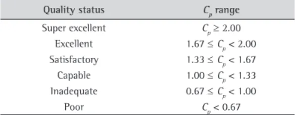
Clearly, the aim of process control is to make Cp as large as possible. The adoption of the Cp index presupposes that the variable θ is normally distributed and that the mean µ^ is equal to the specified target value T. The coefficient Cp is defined as the ratio of the allowable tolerance spread and the actual spread of the data. Table 1 indicates quality status as a function of Cp values, according to Kaya
& Kahraman (2010).
The six-sigma coverage represents the spread of 99.73% of the data in normally distributed processes. In practice, there are cases in which the process is not centred on the target value T, i.e µ≠ T. To avoid such drawback, the index Cpk is defined
ˆ ˆ , 3ˆ 3ˆ
pk
USL LSL
C min
σ σ
µ µ
− −
= (2)
The quality conditions indicated in Table 1 for Cp are also valid for Cpk values. On the other hand, when the distribution of θ is normal and the mean offered to ran some configurations to serve as a data
basis for this application.
4. Process capability indices in thermal
performance analysis
A process capability index is a numerical element that compares the characteristics of a production or servicing process to engineering specifications. A value of such an index equal or larger than a pre-established level indicates that the current process is capable of producing results that, in all likelihood, will meet or exceed the pre-defined requirements. A capability index of this sort is convenient because it reduces complex information about the quality of the process to a single number (Pearn & Lin, 2004; Anis, 2008; Wu et al., 2009; Gonçalez & Werner, 2009). A former application of the PCI methodology in the thermal evaluation of the transport of refrigerated products is described in Estrada-Flores & Eddy (2006).
The starting point of the process capability analysis is the definition of a few measurable properties which can give a significant insight into the quality of the output of the process under consideration. For that, one has to associate a specification interval, that is, an upper specification limit (USL) and a lower specification limit (LSL), to each of the measurements of interest. Of course, some measurement values might be out of the specification limits. Thus, the capability analysis problem consists in the estimation of a statistical model for the process in order to be able to predict the number of points falling out of the specification limits, and therefore giving a measure of the process capability (Bittanti et al., 1998).
Process capability indices (PCI) are frequently used as an integral part of the statistical control of system quality and productivity. The relationship between the actual process performance and the specification limits or tolerance may be quantified using appropriate PCI. They are statistically designed to provide common and easily computed coefficients measured with a dimensionless function of its parameters and specifications. In our application, the analysis of the temperature variability inside a refrigerated vehicle is performed by means of TTI data series collected along typical distribution journeys. Since temperature largely determines the rate of microbial activity, continuous monitoring of the full temperature history usually allows for the adequate control of the process along short and medium distance situations.
Table 1. Quality status and Cp values.
Quality status Cp range
Super excellent Cp≥ 2.00 Excellent 1.67 ≤ Cp < 2.00 Satisfactory 1.33 ≤ Cp < 1.67 Capable 1.00 ≤ Cp < 1.33 Inadequate 0.67 ≤ Cp < 1.00
Poor Cp < 0.67
families of frequency curves to select an adequate probability distribution to that objective. The method of moments is a known approach to the problem of estimating the parameters from a family of frequency curves (Bittanti et al., 1998; Elderton & Johnson, 1969). It is based on the following: given a family of probability distributions which depends on a number of parameters, one can manage to derive close form expressions for the first moments, by applying the operators
( , ) 1, 2,i , ,
f d i n
+∞
−∞
= …
∫
θ ϕ θ θ (6)to the probability density function f (θ, ϕ) of θ, where ϕ∈ Rn is the vector of unknown parameters.
Then, by equating such parametric expressions to the numerical estimates of the moments obtained from the data, one has a set of n equations which can be solved for the n unknown parameters. For common families of distributions, the number of parameters is not very large. Thus, it is usually possible to solve the equations analytically and obtain transformations with the estimated moments as inputs, and the values of the parameters as outputs (Bittanti et al., 1998).
The Pearson system of curves is defined as the set of functions f (θ) satisfying the following differential equation (Bittanti et al., 1998; Elderton
& Johnson, 1969):
(
)
2
0 1 2
( ) ( )
a f df
d b b b
θ θ
θ
θ θ θ
− =
+ + (7)
where a, b0, b1 and b2 are four real parameters. Among the solutions of (7), curves of different kinds can be found, like, for example, bell-shaped, J-shaped or U-shaped distributions. The solution of (7) varies according to the roots of the second order polynomial (Elderton & Johnson, 1969):
2
0 1 2 0
b +bθ+bθ = (8)
As proposed by Pearson, the various forms or curve types can be classified according to the value of the so-called critical element K:
2 1 0 2
4
b K
b b
= (9)
which ranges from –∞ to +∞ and is related to the location of the roots of polynomial (8) in the complex plane.
Another form to express K is (Bittanti et al., 1998)
(
)
2
1 2
2 1 2 1
( 3) 4 4 3 (2 3 6)
K β β
β β β β
+ =
− − − (10)
where
µ^ is centred on the target value T, one has Cp = Cpk. In addition, the index Cpm explicitly considers the distance between the mean and the target value T (Gonçalez & Werner, 2009):
2 2
6 ˆ ( ˆ )
pm
USL LSL C
T
σ µ
− =
+ − (3)
To obtain a capability index more sensitive than Cpk and Cpm, with regard to departures of the process mean µ^ from the target value T, another third generation of capability index Cpmk has been introduced (Gonçalez & Werner, 2009; Chang, 2009):
2 2 2 2
ˆ ˆ
,
ˆ ˆ
3 ˆ ( ) 3 ˆ ( )
pmk
USL LSL
C min
T T
µ µ
µ µ
σ σ
− −
=
+ − + −
(4)
4.2.
Capability analysis of non-normal data
4.2.1.
Clements’ method
When it is detected that the process control variable is not normally distributed, one way to introduce the effects of non-normality into the analysis is Clements’ method, in which the expression (1) is generalized as follows (Bittanti et al., 1998; Gonçalez & Werner, 2009; Hosseinifard et al., 2009):
0.9987 0.0013
, ˆ ˆ
pk
USL LSL
C min
m m
θ θ
µ µ
− −
= − −
(5)
where m is the median of the distribution and
θ0.9987 and θ0.0013are the percentiles corresponding to probabilities 0.9987 and 0.0013, respectively. It is clear that in the normal case this formulation reduces to (2), since then µ^ = m, θ0,0013 = µ^ – 3σ^, and θ0,9987 = µ^ + 3σ^. This nonparametric method seems very attractive because of its simplicity, but unfortunately it suffers from two major drawbacks. First, when working with small samples or noisy data, the nonparametric estimation of tail percentiles becomes a difficult task and the obtained estimates can be very inaccurate. Therefore, this approach is likely to be very sensitive to sampling in actual applications. Second, the estimated percentiles do not provide a very clear picture of the distribution underlying the data. This signifies that it cannot serve for process monitoring, because of its limited ability to detect changes in the process distribution (Bittanti et al., 1998).
4.2.2.
The Pearson system of curves
In our application, the variable θ is not represented by a normal distribution (see Section 6). As indicated in Section 6, the TTI data obtained with the SA meta-heuristic are represented by 394 temperature and time values covering a typical tour, to the exception of the line-haul segment from the last visit to the depot. Computing the central moments of the TTI series, one has m2 = 2.227, m3 = 0.352 and m4 = 22.922, with mean µ = 5.05 °C and skewness = 0.106. Expression (10), associated with (11), yields K = 0.0062 > 0, meaning that the probability distribution of θ is a Pearson’s Type IV curve. The fitting of a distribution such as (14) is not simple and usually requires large samples in order to adequately represent the tail effect in the mathematical representation.
4.2.3.
The Burr transformation approach
Another method of handling non-normal situations in PCI analysis is to reduce the non-normal data into a normal configuration through a transformation technique, and then use a conventional normal method to estimate PCI values (Lin & Chen, 2006). Burr (1973) proposed a system of probability distributions, denominated Burr XII distribution, whose cumulative function is
( )
1 (1 c)k, 0,( )
0 0F x = − +x − forx≥ andF x = for x< (16)
The corresponding probability density function of the Burr XII distribution is (Lin & Chen, 2006)
( )
1(
)
( 1)c 1 c k
f x =k c x − +x − + (17)
Burr (1973) tabulated the expected values, standard deviations, skewness and kurtosis coefficients for the Burr XII distribution, for several combinations of c and k. The resulting tables enable users to make a standardized transformation between a sample variate and a Burr random variate. For a set of data, after the sample skewness and kurtosis coefficients have been estimated, the mean and standard deviation of the corresponding Burr distribution may be obtained using standard tables.
As mentioned, the fitting of probability functions, such as Pearson’s curves and Burr’s distribution, is not simple and usually requires large samples in order to adequately represent the tail effect in the mathematical representation. As a result, several approximate approaches to the PCI problem with skewed populations have been proposed and tested in the literature (Chang & Bai, 2001; Chang et al., 2002; Gonçalez & Werner, 2009).
2
3 4
1 2 2 2
2 2
m m
and
m m
β = β = (11)
m2, m3 and m4 being the second, third and fourth central moments of f (θ).
Pearson defined 13 such types of curves but, for practical applications, three main types are of interest (Bittanti et al., 1998; Elderton & Johnson, 1969):
Pearson’s Type I: Expression (8) has two real
roots of opposite sign, yielding K < 0. The solution of (8) is
( )
1 20
1 2
1 1
f y
g g
θ θ
θ
d d
= + −
(12)
where d1, d2, g1, g2 are coefficients to be fitted to the data and y0 is the normalization factor. The corresponding pdf of (12) only exists when θ is limited to the range
1 2
d θ d
− < < (13)
over which θ is real and positive.
Pearson’s Type IV: It corresponds to values of
K between 0 and 1, i.e. to situations where (8) has two complex conjugate roots, leading to the solution
( )
2 (( ) ( ))/ /
0 1
v arctan v r
v
f y e
r
g
θ d θ
θ
d −
− −
= + −
(14)
where d, ν, r, g are the four parameters to be fitted to the data and y0 is the normalization factor. The range of θ in this case is unlimited, i.e. –∞ < θ <+∞.
Pearson’s Type VI: It corresponds to values of K
greater than one, i.e., to situations where (8) has two real roots of the same sign, leading to the solution
( )
1 20
1 2
1 1
f y
g g
θ θ
θ
d d
= + +
(15)
with the pdf of f (θ) limited to the range d1 < θ <+∞, or –∞ < θ < d2, depending on the sign of the roots of polynomial (8). Thus, while Type I curves are adequate for the representation of variates with both an upper and a lower limit, Type VI curves can be used when only one such limit exists as, for example, the case of a pdf of a nonnegative variable to be fitted to the data (Bittanti et al., 1998). All other Pearson’s curve types, sometimes indicated as transition types, correspond to single values of K. For instance, when K is nil, it indicates that the distribution is symmetrical and, in the Pearson system of frequency curves, it can be the
Normal, the Uniform, the Pearson type II and the
The PCI for temperature θ, for the case of two-side specifications (upper and lower values) is
( ) ( )
{
,}
,(
)
6 6 1
U L
pk pk pk
USL LSL
C min C C min
Pθ Pθ
µ µ σ σ − − = = −
(24)
In Equations 22 and 23, 2σU and 2σL are used in place of σ to reflect the degree of skewness in the probability distribution of θ. When the underlying distribution of θ is symmetric Pθ = 0.5, repeating the
value given by (1). However, if it is skewed, the value of Cpk given by (24) is smaller than the standard one given by (1).
The numerical estimation of Cp and Cpk is performed as follows. Let (θ1, θ2, ..., θn) be the sample containing n values of the temperature θ. The mean
θ^ and the standard deviation σ^ of the sample are computed. The probability Pθ can be estimated by using the number of observations with value smaller than or equal to θ^ (Chang et al., 2002):
1 ) ˆ 1 ( ˆ n i i P g n
θ θ θ
=
≅
∑
− (25)where g(x) = 1 for x ≥ 0 and g(x) = 0 for x < 0. Then Cpk can be estimated by substituting µ^, σ^, and P^θ for µ, σ andPθrespectively in Equation 24.
5. A simulated annealing approach to
solve the vehicle routing problem
Simulated annealing (SA) is a meta-heuristic for solving combinatorial optimization problems. The algorithm is based on a combination of ideas from two different fields: statistical physics (physical annealing process of solids converging to their minimum energy states) and combinatorial optimization (Kirkpatrick et al., 1983; Magalhães
& Moura Neto, 2011). The simulated annealing
algorithm starts off with a given initial solution, very often chosen at random, and continuously tries to move from a current solution to one of its neighbours by applying a generation mechanism and an acceptance criterion. The acceptance criterion allows for sporadic deteriorations in the optimization function in a limited way. This is controlled by a parameter that plays a similar role as the temperature in the physical annealing process. The possibility of deteriorations makes the SA algorithm more general than pure iterative improvement algorithms, in which only strict improvements are applied. The resulting effect is that the annealing algorithm can systematically avoid local minima in order to arrive at a global minimum.
Many works have been published on SA applications to the solution of vehicle routing
4.3.
An approximate C
pkevaluation method
Gonçalez & Werner (2009) compared a number of approximate methods to evaluate non-normal situations and suggested that the method of Chen & Ding (2001) reflects with better accuracy the number of normal non-conforming items in the evaluated sample, being superior to the other analysed methods. Such method adjusts the values of PCIs in accordance to the degree of skewness of the underlying population, by using specific factors in computing the deviations above and below the variable mean.
The method is based on the idea that σ can be divided into upper and lower deviations, σU and σL, which represent the dispersions of the upper and lower sides around the mean µ, respectively. An asymmetric probability density function f (θ) can be approximated with two normal pdfs
( )
1( )
1
2 2 2 2
U L
U U L L
f θ θ µ and f θ θ µ
σ σ σ σ
− −
= ∅ = ∅
(18)
with the same mean µ but different standard deviations 2σU and 2σL, where ∅ represents the standard normal pdf. The upper and lower sides of f (θ) are approximated with the upper side of fU (θ) and the lower side of fL (θ), respectively. The values of σU and σL are computed as Chang et al., 2002)
(
1)
U Pθ and L Pθ
σ = σ σ = − σ (19)
with Pθ = Pr{θ < µ}.
The value of Cp is defined as (Chang & Bai, 2001)
)
, ,
6 2 6 2 6 2 6 2(1 )
1 1
,
6 2 2(1
p
U L
USL LSL USL LSL USL LSL USL LSL
C min min
P P USL LSL min P P θ θ θ θ
σ σ σ σ
σ − − − − = × × = × × − = − = − (20)
Making Dθ = 1 + |1 – 2Pθ|, expression (20) can be simplified to
1 6 p USL LSL C Dθ σ −
= (21)
where 1/Dθ is a corrective coefficient on (1) due to the skewness of the probability distribution of θ. On the other hand, according to Chang et al. (2002), the value of Cpk, corrected for skewness, can be estimated as follows. First, the upper and lower capability indices are defined as
( )
3 2 6
U pk U USL USL C Pθ µ µ σ σ − − = =
× (22)
( )
3 2 6 (1 )
L pk L LSL LSL C Pθ µ µ σ σ − − = =
distance, but at same time keeping the TTI values within the required range. The TTI results from the SA model are represented by 394 temperature and time values, covering a typical tour. Figure 2 depicts the histogram of the TTI values obtained with the SA meta-heuristic. It can be seen that the temperature distribution is positively skewed (not normal), justifying the use of the Cpk index (see Section 4).
The TTI data used to make Figure 2 do not include the values corresponding to the vehicle travel from the last visit back to the depot because, in this application, the truck travels empty along the backwards line-haul segment of the route since all cargo has been delivered up to that point, and therefore the corresponding temperature values do not affect the product quality. The mean temperature is µ^ = 5.05 °C, and its standard deviation σ^ = 1.49. problems (Breedam, 1995; Osman, 1993; Mauri &
Lorena, 2009; Leung et al., 2013). In this paper, SA has been applied to solve the optimization of the proposed vehicle routing problem. Let n be the number of delivering points (clients) to be visited in the route. Each client receives an identification number i = 1, 2, …, n. Putting the client numbers according to the sequence they are visited, one has a vector of n components. The depot is part of the Hamiltonian routing cycle, and is placed in position n + 1 on such a vector. In the application, two exploratory stages, represented by k, are considered. In stage k = 1, a candidate solution, represented by the vector x, is defined by a Monte Carlo routine, with the position of each client in the visiting sequence selected at random. This is done to allow the SA procedure to explore prospective solutions covering all the set of possibilities, thus avoiding local minima. In stage 2, the selection of a new candidate solution is performed in a more restricted manner. In order to get a candidate solution departing from a former solution, two clients are selected at random in the corresponding vector. The positions of these two clients are exchanged mutually in order to generate a new prospective solution, with the remaining clients keeping the same positions they occupied before. With this approach the SA improvement sequence explores closer neighbouring possibilities, thus avoiding too large jumps over the overall set of solutions.
6. Results and sensitivity analysis
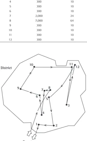
The necessary basic inputs for the model application are presented in Table 2.The urban distribution district in this work is located about 84 km from the base depot. The served urban district has an approximated area of 73 sq.km, where 12 retail shops are located, as shown in Figure 1. The product is ready-to-eat refrigerated meat products (ham, turkey and chicken breasts, salami, sausage). A total of 12,000 kg of assorted products are distributed in the daily round, with two retailers receiving larger quantities (7,000 and 2,000 kg respectively), while the other ten clients getting 300 kg each (Table 2). The route starts with a line-haul phase, which goes from the depot to the first client in the district, and taking 84 minutes approximately. It is followed by a sequence of visits, intercalating cargo discharging tasks with vehicle displacements between successive delivery points. Finally, there is the line-haul reverse segment, linking the last served client to the depot.
The optimal delivery sequence shown in Figure 1 was obtained with the SA algorithm, in which the objective is to minimize the vehicle travelling
Figure 1. The simulated annealing (SA) optimized route.
Table 2. Product quantity delivered per retailer client and mean unloading time.
Retailer number
Quantity of product delivered per visit (kg)
Mean unloading time (min)
1 300 10
2 300 10
3 300 10
4 300 10
5 300 10
6 300 10
7 2,000 24
8 7,000 64
9 300 10
10 300 10
11 300 10
is even worse, with Cpk = 0.15. Looking at the zigzag sequence pattern of the SA solution (Figure 1), it might look non intuitive, but the increased distances linking some servicing points can help the vehicle refrigeration equipment to reduce the internal temperature to acceptable levels. In fact, the temperature inside the truck along the delivery journey tends to increase when it stops to discharge the product, and the temperature inversely tends to decrease while the vehicle is travelling from a client to the next one in the routing sequence. Generally, a heavier discharge weight takes more time to be unloaded. If the next visiting point is located close by, the corresponding travelling time might be too short, and the temperature would not decrease enough to compensate for the heat surge observed in the last unloading stops. This means that the vehicle routing sequence has an important influence in the TTI history, indicating that both have to be investigated jointly, as it has been done in this analysis.
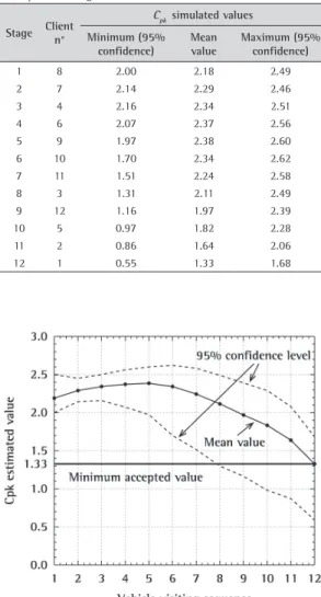
For the SA optimal solution indicated above, the values of Cpk were also computed considering the intermediate stages of the process. The process stages correspond to the instants when the vehicle has just finished a delivery service to a client, and is preparing to depart for the next visit. In order to investigate the sensitivity of these results, a simulation was performed considering the product discharging times and the vehicle travelling times as random variables. For this, such variables were assumed to be log-normally distributed. It was assumed a coefficient of variation CV = 0.2 for the cargo discharging times, and CV = 0.05 for all vehicle In this application there is no target value for
the temperature θ, being only necessary to respect the two-sided specified limits, namely LSL and USL, whose values are LSL = 2 °C and USL = 7 °C in our analysis. Consequently, as indicated in Section 4.1, the index Cpk has been adopted. In the sequel, the capability index Cpk is computed for every route sequence following the Chen & Ding (2001) method described in Section 4.3, since it is computationally easy to implement and has shown to be superior when compared to other approximate PCI methods (Gonçalez & Werner, 2009). Although, in some manufacturing processes, values of Cpk greater than 1.33 are adopted, a capable level, corresponding to a six-sigma formulation (see Table 1), seems more appropriate for this kind of process, since many external factors generate greater dispersions in the operational variables. Other authors, such Estrada-Flores & Eddy (2006), analysing a similar problem, have adopted the same Cpk threshold.
The computer model (steps c and d, Section 2) was programmed in Free Pascal, version 2.6.4, to be further incorporated into a Delphi format. Applying the SA algorithm, the first stage involved 1,306 steps, and the second 10,815 steps, leading to the following optimal delivery sequence: Depot – 8 - 7 – 4 – 6 – 9 – 10 – 11 – 3 – 12 – 5 – 2 – 1 – Depot, with a total vehicle distance of 222.7 km, and with a satisfactory “capable” Cpk value of 1.33.
the local links between clients in the route, show comparatively less variation.
Figure 3 shows that, for this application and with a 95% confidence level, the four last visits indicated in Table 3, namely clients 12, 5, 2, and 1, should be assigned to another truck. In fact, a better approach to set the process within the specified temperature range should be the re-assignment of delivery stops per vehicle round, with the selection of smaller vehicles to perform the tasks defined with the aid of an optimization algorithm.
Although food temperature control largely influences microbial activities, allowing for an adequate surveillance of product quality along short and medium distance delivery routes, new risks of foodborne illnesses associated with micro-organisms are presently identified. One factor is the changing characteristics of the relevant micro-organisms. Second, the occurrence of changing production methodologies, in parallel with changes in the environment and an increase of the global trade of food stuffs (Havelaar et al., 2010). In parallel, it can be noticed in the literature substantial advances in the development of predictive microbiology, with efforts exploring a better balance between science and applications (McMeekin et al., 2008). Since temperature abuses in the distribution of refrigerated and frozen products are quite common in developing countries like Brazil (Pereira et al., 2010), its correct monitoring is naturally a first step in establishing a more comprehensive food perishability control, as is the case of the present work. Following this line further, the authors intend to research on the distribution of refrigerated products applying mathematical models describing the effects of environmental conditions on the growth and inactivation of microorganisms, in food distribution under more diverse logistics conditions.
7. Conclusions
The investigation presented in this paper has shown that the assignment of refrigerated vehicles to the distribution of perishable products is not a trivial process, requiring, in fact, a more detailed and integrated investigation of its thermal aspects. The use of process capability index evaluation over TTI data, together with a simulating annealing algorithm has produced an optimal constrained result in terms of a minimum-distance distribution route, but at same time respecting a pre-defined quality requirement, expressed through a Cpk coefficient. travel times, including the line-haul segment and the
local vehicle displacements, represented by the links from one served client to the next. For each stage, the simulation was replicated 1,000 times. The results are shown in Table 3 and Figure 3, where the mean Cpk values are exhibited, as well as their lower and upper 95% significance levels.
The results of the model show that the thermal properties inside the vehicle are very sensitive to time variations along the route, specifically the cargo discharging times. This fact has practical implications in real-life operations because different delays are common as, for example, unexpected waiting times to start the unloading process, long paths to reach the point where the discharged cargo is to be set inside the client’s premises, excessive product checking times, etc. And conversely, vehicle travelling times, both along the line-haul segments and along
Table 3. Optimal simulated annealing route: Cpk values for
each process stage.
Stage Client
n°
Cpk simulated values
Minimum (95% confidence)
Mean value
Maximum (95% confidence)
1 8 2.00 2.18 2.49
2 7 2.14 2.29 2.46
3 4 2.16 2.34 2.51
4 6 2.07 2.37 2.56
5 9 1.97 2.38 2.60
6 10 1.70 2.34 2.62
7 11 1.51 2.24 2.58
8 3 1.31 2.11 2.49
9 12 1.16 1.97 2.39
10 5 0.97 1.82 2.28
11 2 0.86 1.64 2.06
12 1 0.55 1.33 1.68
Estrada-Flores, S., & Eddy, A. (2006). Thermal performance indicators for refrigerated road vehicles. International Journal of Refrigeration, 29, 889-898. http://dx.doi. org/10.1016/j.ijrefrig.2006.01.012
Flick, D., Hoang, H. M., Alvarez, G., & Laguerre, O. (2012). Combined deterministic and stochastic approaches for modelling the evolution of food products along the cold chain. Part I: Methodology. International Journal of Refrigeration, 35, 907-914. http://dx.doi.org/10.1016/j. ijrefrig.2011.12.010
Food Refrigeration & Process Engineering Research Centre – FRPERC (2000). Coolvan Manual (Version 3.0). University of Bristol, UK.
Giannakourou, M. C., & Taoukis, P. S. (2003). TTI-based distribution management system for quality optimization of frozen vegetables at the consumer end. Journal of Food Science, 68, 201-209. http://dx.doi. org/10.1111/j.1365-2621.2003.tb14140.x
Giannakourou, M. C., Koutsoumanis, K., Nychas, G. J., &
Taoukis, P. S. (2005). Field evaluation of the application of time temperature integrators for monitoring fish quality in the chill chain. International Journal of Food Microbiology, 102, 323-336. PMid:16014299. http:// dx.doi.org/10.1016/j.ijfoodmicro.2004.11.037
Gigiel, A. J., James S. J., & Evans, J. A. (1998). Controlling temperature during distribution and retail. In Proceedings 3rd Karlsruhe Nutrition Symposium,
Karlsruhe, Germany.
Gonçalez, P. U., & Werner, L. (2009). Comparação dos índices de capacidade do processo para distribuições não-normais. Gestão & Produção, 16(1), 121-132. http:// dx.doi.org/10.1590/S0104-530X2009000100012 Havelaar, A. H., Brul, S., De Jong, A., De Jonge, R., Zietering,
M. H., & Ter Kuile, B. (2010). Future challenges to microbial food safety. International Journal of Food Microbiology, 139, S79-S94. PMid:19913933. http:// dx.doi.org/10.1016/j.ijfoodmicro.2009.10.015
Hosseinifard, S. Z., Abassi, B., Ahmad, S., & Abdollahian, M. (2009). A transformation technique to estimate the process capability index for non-normal data. The International Journal of Advanced Manufacturing Technology, 40, 512-517. http://dx.doi.org/10.1007/ s00170-008-1376-x
Hsu, C. I., Hung, S. F., & Li, H. C. (2007). Vehicle routing problem with time-windows for perishable food delivery. Journal of Food Engineering, 80, 465-475. http://dx.doi. org/10.1016/j.jfoodeng.2006.05.029
James, S. J., & James, C. (2010). The cold chain and climate change. Food Research International, 43, 1944-1956. http://dx.doi.org/10.1016/j.foodres.2010.02.001 James, S. J., James, C., & Evans, J. A. (2006). Modelling of
food transportation systems – a review. International Journal of Refrigeration, 29, 947-957. http://dx.doi. org/10.1016/j.ijrefrig.2006.03.017
Jedermann, R., Ruiz-Garcia, L., & Lang, W. (2009). Spatial temperature profiling by semi-passive RFID loggers for perishable food transportation. Computers and Electronics in Agriculture, 65(2), 145-154. http://dx.doi. org/10.1016/j.compag.2008.08.006
Kaya, I., & Kahraman, C. (2010). A new perspective on fuzzy process capability indices: Robustness. Expert Systems with Applications, 37, 4593-4600. http://dx.doi. org/10.1016/j.eswa.2009.12.049
References
Amorim, P., Günther, H. O., & Almada-Lobo, B. (2012). Multi-objective integrated production and distribution planning of perishable products. International Journal of Production Economics, 138, 89-101. http://dx.doi. org/10.1016/j.ijpe.2012.03.005
Anis, M. Z. (2008). Basic process capability indices: An expository review. International Statistical Review, 76, 347-367. http://dx.doi.org/10.1111/j.1751-5823.2008.00060.x
Azi, N., Gendreau, M., & Potvin, J. Y. (2007). An exact
algorithm for a simple-vehicle routing problem with time windows and multiple routes. European Journal of Operational Research, 178, 755-766. http://dx.doi. org/10.1016/j.ejor.2006.02.019
Barriga, G. D. C., Ho, L. L., & Borges, W. S. (2003). Process capability index for one-sided specification limit. Production, 13, 40-49.
Bittanti, S., Lovera, M., & Moiraghi, L. (1998). Application of non-normal process capability indices to semiconductor quality control. IEEE Transactions on Semiconductor Manufacturing, 11, 296-303. http://dx.doi. org/10.1109/66.670179
Borch, E., & Arinder, P. (2002). Bacteriological safety issues in red meat and ready-to-eat meat products, as well as control measures. Meat Science, 62, 381-390. http:// dx.doi.org/10.1016/S0309-1740(02)00125-0
Breedam, A. V. (1995). Improvement heuristics for the vehicle routing problem based on simulated annealing. European Journal of Operational Research, 86, 480-490. http://dx.doi.org/10.1016/0377-2217(94)00064-J Bulba, E. A., & Ho, L. L. (2004). Capability index for linear
and non-linear functions. Production, 14, 6-11. Burr, I. W. (1973). Parameters for a general system of
distributions to match a grid of a3 and a4. Communications in Statistics – Theory and Methods, 2, 1-21.
Chang, Y. S. (2009). Interval estimation of capability index Cpmk for manufacturing processes with asymmetric tolerances. Computers & Industrial Engineering, 56, 312-322. http://dx.doi.org/10.1016/j.cie.2008.06.004 Chang, Y. S., & Bai, D. S. (2001). Control charts for
positively-skewed populations with weighted standard deviations. Quality and Reliability Engineering International, 17, 397-406. http://dx.doi.org/10.1002/ qre.427
Chang, Y. S., Choi, I. S., & Bai, D. S. (2002). Process capability indices for skewed populations. Quality and Reliability Engineering International, 18, 383-393. http://dx.doi. org/10.1002/qre.489
Chen, H. K., Hsueh, C. F. & Chang, M. S. (2009). Production scheduling and vehicle routing with time windows for perishable food products. Computers & Operations Research, 36, 2311-2319. http://dx.doi.org/10.1016/j. cor.2008.09.010
Chen, J. P. & Ding, C. G. (2001). A new process capability index for non-normal distributions. The International of Quality and Reliability Management, 18, 762-770. http://dx.doi.org/10.1108/02656710110396076
Elderton, W. P., & Johnson, N. L. (1969). Systems of
Pereira, V. F., Dória, E. C. B, Carvalho Júnior, B. C., Neves
Filho, L. C., & Silveira Júnior, V. (2010). Avaliação de temperaturas em câmaras frigoríficas de transporte urbano de alimentos resfriados e congelados. Ciência e Tecnologia de Alimentos, 30, 158-165. http://dx.doi. org/10.1590/S0101-20612010000100024
Sahin, E., Babaï, M. Z., Dallery, Y., & Vaillant, R. (2007). Ensuring supply chain safety through time temperature integrators. International Journal of Logistics Management, 18, 102-124. http://dx.doi. org/10.1108/09574090710748199
Simpson, R., Almonacid, S., Nuñez, H., Pinto, M., Abakarov,
A., & Teixeira, A. (2012). Time-temperature indicator to monitor cold chain distribution of fresh salmon (salmo salar). Journal of Food Process Engineering, 35, 742-750. http://dx.doi.org/10.1111/j.1745-4530.2010.00623.x Smolander, M., Alakomi, H.-L., Ritvanen, T., Vainionpää,
J., & Ahvenainen, R. (2004). Monitoring of the quality of modified atmosphere packaged broiler chicken cuts stored in different temperature conditions. A. Time-temperature indicators as quality-indicating tools. Food Control, 15, 217-229. http://dx.doi.org/10.1016/S0956-7135(03)00061-6
Syslo, M. M., Deo, N., & Kowalik, J. S. (2006). Discrete
Optimization Algorithms with Pascal Programs. Mineola: Dover Publications.
Tarantilis, C. D., & Kiranoudis, C. T. (2002). Distribution of fresh meat. Journal of Food Engineering, 51, 85-91. http://dx.doi.org/10.1016/S0260-8774(01)00040-1 Tso, C. P., Yu, S. C. M., Poh, H. J., & Jolly, P. G. (2002).
Experimental study on the heat and mass transfer characteristics in a refrigerated truck. International Journal of Refrigeration, 25, p. 340-350. http://dx.doi. org/10.1016/S0140-7007(01)00015-9
Wu, C. W., Pearn, W. L., & Kotz, S. (2009). An overview of theory and practice on process capability indices for quality assurance. International Journal of Production Economics, 117, 338-359. http://dx.doi.org/10.1016/j. ijpe.2008.11.008
Acknowledgments
This research has been supported by Capes Foundation (Brazil) and DFG - German Research Foundation, Bragecrim Project n° 2009-2, with the partnership of BIBA – Bremer Institut für Produktion und Logistik, Universität Bremen, Germany.
Kirkpatrick, S., Gellat, C. D., & Vecchi, M. P. (1983). Optimization by simulated annealing. Science, 220, 671-680. PMid:17813860. http://dx.doi.org/10.1126/ science.220.4598.671
Leung, S. C. H., Zhang, Z., Zhang, D., Hua, X., & Lim, M. K. (2013). A meta-heuristic algorithm for heterogeneous fleet routing problems with two-dimensional loading constraints. European Journal of Operational Research, 225, 199-210. http://dx.doi.org/10.1016/j. ejor.2012.09.023
Lin, P. H., & Chen, F. L. (2006). Process capability analysis of non-normal process data using the Burr XII distribution. The International Journal of Advanced Manufacturing Technology, 27, 975-984. http://dx.doi.org/10.1007/ s00170-004-2263-8
Magalhães, M. S., & Moura Neto, F. D. (2011).
Economic-statistical design of variable parameters non-central chi-square control chart. Production, 21, 259-270.
Mauri, G. R., & Lorena, L. A. N. (2009). A new approach for
the dial-a-ride problem. Production, 19, p. 41-54. McMeekin, T., Bowman, J., McQuestin, O., Mellefont, L.,
Ross, T., & Tamplin, M. (2008). The future of predictive microbiology: Strategic research, innovative applications and great expectations. International Journal of Food Microbiology, 128, 2-9. PMid:18703250. http://dx.doi. org/10.1016/j.ijfoodmicro.2008.06.026
Mingoti, S. A., & Glória, F. F. F. (2008). Comparing Mingoti
and Glória’s and Niverthi and Dey’s multivariate capability
indexes. Production, 18, 598-608.
Mingoti, S. A., Oliveira, F. L. P., & Conceição, M. M. C. (2011). Capability indices for independent multivariate
processes: extensions of Niverthi and Dey’s and Mingoti
and Glória’s indices. Production, 21, 94-105.
Moureh, J., & Derens, E. (2000). Numerical modelling of
the temperature increase in frozen food packaged in pallets in the distribution chain. International Journal of Refrigeration, 23, 540-552. http://dx.doi.org/10.1016/ S0140-7007(99)00081-X
Osman, I. H. (1993). Metastrategy simulated annealing and tabu search algorithms for the vehicle routing problem. Annals of Operations Research, 41(4), 421-451. http:// dx.doi.org/10.1007/BF02023004
Oswald, A., & Stirn, L. Z. (2008). A vehicle routing algorithm for the distribution of fresh vegetables and similar perishable food. Journal of Food Engineering, 85, 285-295. http://dx.doi.org/10.1016/j.jfoodeng.2007.07.008 Pearn, W. L., & Lin, P. C. (2004). Testing process performance