Iterative Methods for Sparse Linear Systems

(1)

Iterative Methods

for Sparse

Linear Systems

Second Edition

0.10E-06 0.19E+07

Yousef Saad

(2)

(3)

Preface to the second edition

In the six years that passed since the publication of the first edition of this book, iterative methods for linear systems have made good progress in scientific and engi-neering disciplines. This is due in great part to the increased complexity and size of the new generation of linear and nonlinear systems which arise from typical appli-cations. At the same time, parallel computing has penetrated the same application areas, as inexpensive computer power became broadly available and standard com-munication languages such as MPI gave a much needed standardization. This has created an incentive to utilize iterative rather than direct solvers because the prob-lems solved are typically from 3-dimensional models for which direct solvers often become ineffective. Another incentive is that iterative methods are far easier to im-plement on parallel computers,

Though iterative methods for linear systems have seen a significant maturation, there are still many open problems. In particular, it still cannot be stated that an arbitrary sparse linear system can be solved iteratively in an efficient way. If physical information about the problem can be exploited, more effective and robust methods can be tailored for the solutions. This strategy is exploited by multigrid methods. In addition, parallel computers necessitate different ways of approaching the problem and solution algorithms that are radically different from classical ones.

Several new texts on the subject of this book have appeared since the first edition. Among these, are the books by Greenbaum [154], and Meurant [209]. The exhaustive 5-volume treatise by G. W. Stewart [274] is likely to become the de-facto reference in numerical linear algebra in years to come. The related multigrid literature has also benefited from a few notable additions, including a new edition of the excellent “Multigrid tutorial” [65], and a new title by Trottenberg et al. [286].

Most notable among the changes from the first edition, is the addition of a sorely needed chapter on Multigrid techniques. The chapters which have seen the biggest changes are Chapter 3, 6, 10, and 12. In most cases, the modifications were made to update the material by adding topics that were developed recently or gained impor-tance in the last few years. In some insimpor-tances some of the older topics were removed or shortened. For example the discussion on parallel architecture has been short-ened. In the mid-1990’s hypercubes and “fat-trees” were important topic to teach. This is no longer the case, since manufacturers have taken steps to hide the topology from the user, in the sense that communication has become much less sensitive to the

(12)

underlying architecture.

The bibliography has been updated to include work that has appeared in the last few years, as well as to reflect change of emphasis when new topics have gained importance. Similarly, keeping in mind the educational side of this book, many new exercises have been added. The first edition suffered many typographical errors which have been corrected. Many thanks to those readers who took the time to point out errors.

I would like to reiterate my thanks to all my colleagues who helped make the the first edition a success (see the preface to the first edition). I received support and encouragement from many students and colleagues to put together this revised volume. I also wish to thank those who proofread this book. I found that one of the best way to improve clarity is to solicit comments and questions from students in a course which teaches the material. Thanks to all students in Csci 8314 who helped in this regard. Special thanks to Bernie Sheeham, who pointed out quite a few typographical errors and made numerous helpful suggestions.

My sincere thanks to Michele Benzi, Howard Elman, and Steve Mc Cormick for their reviews of this edition. Michele proof-read a few chapters thoroughly and caught a few misstatements. Steve Mc Cormick’s review of Chapter 13 helped ensure that my slight bias for Krylov methods (versus multigrid) was not too obvious. His comments were at the origin of the addition of Section 13.7 (Multigrid vs Krylov methods).

(13)

PREFACE xv

Suggestions for teaching

This book can be used as a text to teach a graduate-level course on iterative methods for linear systems. Selecting topics to teach depends on whether the course is taught in a mathematics department or a computer science (or engineering) department, and whether the course is over a semester or a quarter. Here are a few comments on the relevance of the topics in each chapter.

For a graduate course in a mathematics department, much of the material in Chapter 1 should be known already. For non-mathematics majors most of the chap-ter must be covered or reviewed to acquire a good background for lachap-ter chapchap-ters. The important topics for the rest of the book are in Sections: 1.8.1, 1.8.3, 1.8.4, 1.9, 1.11. Section 1.12 is best treated at the beginning of Chapter 5. Chapter 2 is essen-tially independent from the rest and could be skipped altogether in a quarter session, unless multigrid methods are to be included in the course. One lecture on finite dif-ferences and the resulting matrices would be enough for a non-math course. Chapter 3 aims at familiarizing the student with some implementation issues associated with iterative solution procedures for general sparse matrices. In a computer science or engineering department, this can be very relevant. For mathematicians, a mention of the graph theory aspects of sparse matrices and a few storage schemes may be sufficient. Most students at this level should be familiar with a few of the elementary relaxation techniques covered in Chapter 4. The convergence theory can be skipped for non-math majors. These methods are now often used as preconditioners and this may be the only motive for covering them.

Chapter 5 introduces key concepts and presents projection techniques in gen-eral terms. Non-mathematicians may wish to skip Section 5.2.3. Otherwise, it is recommended to start the theory section by going back to Section 1.12 on general definitions on projectors. Chapters 6 and 7 represent the heart of the matter. It is recommended to describe the first algorithms carefully and put emphasis on the fact that they generalize the one-dimensional methods covered in Chapter 5. It is also important to stress the optimality properties of those methods in Chapter 6 and the fact that these follow immediately from the properties of projectors seen in Section 1.12. Chapter 6 is rather long and the instructor will need to select what to cover among the non-essential topics as well as topics for reading.

When covering the algorithms in Chapter 7, it is crucial to point out the main differences between them and those seen in Chapter 6. The variants such as CGS, BICGSTAB, and TFQMR can be covered in a short time, omitting details of the algebraic derivations or covering only one of the three. The class of methods based on the normal equation approach, i.e., Chapter 8, can be skipped in a math-oriented course, especially in the case of a quarter system. For a semester course, selected topics may be Sections 8.1, 8.2, and 8.4.

(14)

The rest could be skipped in a quarter course.

Chapter 11 may be useful to present to computer science majors, but may be skimmed through or skipped in a mathematics or an engineering course. Parts of Chapter 12 could be taught primarily to make the students aware of the importance of “alternative” preconditioners. Suggested selections are: 12.2, 12.4, and 12.7.2 (for engineers).

Chapters 13 and 14 present important research areas and are primarily geared to mathematics majors. Computer scientists or engineers may cover this material in less detail.

To make these suggestions more specific, the following two tables are offered as sample course outlines. Numbers refer to sections in the text. A semester course represents approximately 30 lectures of 75 minutes each whereas a quarter course is approximately 20 lectures of 75 minutes each. Different topics are selected for a mathematics course and a non-mathematics course.

Semester course

Weeks Mathematics Computer Science / Eng.

1.9 –1.13 1.1 – 1.6 (Read) ; 1.7; 1.9;

1 – 3 2.1 – 2.5 1.11; 1.12; 2.1 – 2.2

3.1 – 3.3 3.1 – 3.6

4.1 – 4.2 4.1 – 4.2.1; 4.2.3

4 – 6 5. 1 – 5.3; 6.1 – 6.4 5.1 – 5.2.1; 5.3

6.5.1; 6.5.3 – 6.5.9 6.1 – 6.4; 6.5.1 – 6.5.5

6.6 – 6.8 6.7.1 6.8–6.9

7 – 9 6.9 – 6.11; 7.1 – 7.3 6.11.3; 7.1 – 7.3 7.4.1; 7.4.2; 7.4.3 (Read) 7.4.1 – 7.4.2; 7.4.3 (Read)

8.1; 8.2 ; 9.1 – 9.4; 8.1 – 8.3; 9.1 – 9.3 10 – 12 10.1 – 10.3; 10.4.1; 10.1 – 10.3 ; 10.4.1 – 10.4.3;

10.5.1 – 10.5.7 10.5.1 – 10.5.4; 10.5.7

12.2 – 12.4 11.1 – 11.4 (Read); 11.5 – 11.6

13 – 15 13.1 – 13.5 12.1 – 12.2 ; 12.4 – 12.7

(15)

PREFACE xvii

Quarter course

Weeks Mathematics Computer Science / Eng.

1 – 2 1.9 – 1.13 1.1 – 1.6 (Read); 3.1 – 3.5

4.1 – 4.2; 5.1 – 5.4 4.1; 1.12 (Read)

3 – 4 6.1 – 6.4 5.1 – 5.2.1; 5.3

6.5.1; 6.5.3 – 6.5.5 6.1 – 6.3

5 – 6 6.7.1; 6.11.3; 7.1 – 7.3 6.4; 6.5.1; 6.5.3 – 6.5.5 7.4.1 – 7.4.2; 7.4.3 (Read) 6.7.1; 6.11.3; 7.1 – 7.3

7 – 8 9.1 – 9.3 7.4.1 – 7.4.2 (Read); 9.1 – 9.3 10.1 – 10.3; 10.5.1; 10.5.7 10.1 – 10.3; 10.5.1; 10.5.7

(16)

(17)

Preface to the first edition

Iterative methods for solving general, large sparse linear systems have been gain-ing popularity in many areas of scientific computgain-ing. Until recently, direct solution methods were often preferred to iterative methods in real applications because of their robustness and predictable behavior. However, a number of efficient iterative solvers were discovered and the increased need for solving very large linear systems triggered a noticeable and rapid shift toward iterative techniques in many applica-tions.

This trend can be traced back to the 1960s and 1970s when two important de-velopments revolutionized solution methods for large linear systems. First was the realization that one can take advantage of “sparsity” to design special direct meth-ods that can be quite economical. Initiated by electrical engineers, these “direct sparse solution methods” led to the development of reliable and efficient general--purpose direct solution software codes over the next three decades. Second was the emergence of preconditioned conjugate gradient-like methods for solving linear systems. It was found that the combination of preconditioning and Krylov subspace iterations could provide efficient and simple “general-purpose” procedures that could compete with direct solvers. Preconditioning involves exploiting ideas from sparse direct solvers. Gradually, iterative methods started to approach the quality of di-rect solvers. In earlier times, iterative methods were often special-purpose in nature. They were developed with certain applications in mind, and their efficiency relied on many problem-dependent parameters.

Now, three-dimensional models are commonplace and iterative methods are al-most mandatory. The memory and the computational requirements for solving three-dimensional Partial Differential Equations, or two-three-dimensional ones involving many degrees of freedom per point, may seriously challenge the most efficient direct solvers available today. Also, iterative methods are gaining ground because they are easier to implement efficiently on high-performance computers than direct methods.

My intention in writing this volume is to provide up-to-date coverage of itera-tive methods for solving large sparse linear systems. I focused the book on practical methods that work for general sparse matrices rather than for any specific class of problems. It is indeed becoming important to embrace applications not necessar-ily governed by Partial Differential Equations, as these applications are on the rise.

(18)

Apart from two recent volumes by Axelsson [14] and Hackbusch [163], few books on iterative methods have appeared since the excellent ones by Varga [293]. and later Young [322]. Since then, researchers and practitioners have achieved remarkable progress in the development and use of effective iterative methods. Unfortunately, fewer elegant results have been discovered since the 1950s and 1960s. The field has moved in other directions. Methods have gained not only in efficiency but also in robustness and in generality. The traditional techniques which required rather com-plicated procedures to determine optimal acceleration parameters have yielded to the parameter-free conjugate gradient class of methods.

The primary aim of this book is to describe some of the best techniques available today, from both preconditioners and accelerators. One of the aims of the book is to provide a good mix of theory and practice. It also addresses some of the current research issues such as parallel implementations and robust preconditioners. The emphasis is on Krylov subspace methods, currently the most practical and common group of techniques used in applications. Although there is a tutorial chapter that covers the discretization of Partial Differential Equations, the book is not biased toward any specific application area. Instead, the matrices are assumed to be general sparse, possibly irregularly structured.

The book has been structured in four distinct parts. The first part, Chapters 1 to 4, presents the basic tools. The second part, Chapters 5 to 8, presents projection meth-ods and Krylov subspace techniques. The third part, Chapters 9 and 10, discusses preconditioning. The fourth part, Chapters 11 to 13, discusses parallel implementa-tions and parallel algorithms.

Acknowledgments

I am grateful to a number of colleagues who proofread or reviewed different ver-sions of the manuscript. Among them are Randy Bramley (University of Indiana at Bloomingtin), Xiao-Chuan Cai (University of Colorado at Boulder), Tony Chan (University of California at Los Angeles), Jane Cullum (IBM, Yorktown Heights), Alan Edelman (Massachussett Institute of Technology), Paul Fischer (Brown Univer-sity), David Keyes (Old Dominion UniverUniver-sity), Beresford Parlett (University of Cali-fornia at Berkeley) and Shang-Hua Teng (University of Minnesota). Their numerous comments, corrections, and encouragements were a highly appreciated contribution. In particular, they helped improve the presentation considerably and prompted the addition of a number of topics missing from earlier versions.

(19)

PREFACE xxi

Ahmed Sameh for his encouragements and for fostering a productive environment in the department. Finally, I am grateful to the National Science Foundation for their continued financial support of my research, part of which is represented in this work.

(20)

(21)

Chapter 1 BACKGROUND IN LINEAR ALGEBRA

This chapter gives an overview of the relevant concepts in linear algebra which are useful in later chapters. It begins with a review of basic matrix theory and introduces the elementary notation used throughout the book. The convergence analysis of iterative methods requires a good level of knowledge in mathematical analysis and in linear algebra. Traditionally, many of the concepts presented specifically for these analyses have been geared toward matrices arising from the discretization of Partial Differential Equations and basic relaxation-type methods. These concepts are now becoming less important because of the trend toward projection-type methods which have more robust convergence properties and require different analysis tools. The material covered in this chapter will be helpful in establishing some theory for the algorithms and defining the notation used throughout the book.

1.1 Matrices

For the sake of generality, all vector spaces considered in this chapter are complex, unless otherwise stated. A complexn×mmatrixAis ann×marray of complex numbers

aij, i= 1, . . . , n, j = 1, . . . , m.

The set of alln_×mmatrices is a complex vector space denoted byCn×m_{. The main}

operations with matrices are the following:

• Addition:C=A+B, whereA, B, andCare matrices of sizen_×mand

cij =aij +bij, i= 1,2, . . . n, j = 1,2, . . . m.

• Multiplication by a scalar:C=αA, where

cij =α aij, i= 1,2, . . . n, j= 1,2, . . . m.

(22)

• Multiplication by another matrix:

C =AB,

whereA_∈Cn×m_{, B}_∈Cm×p_{, C} _∈Cn×p_{, and}

cij = m

X

k=1

aikbkj.

Sometimes, a notation with column vectors and row vectors is used. The column vectora_∗jis the vector consisting of thej-th column ofA,

a_∗j =



  

a1j

a2j

.. .

anj



  .

Similarly, the notationai∗will denote thei-th row of the matrixA

ai∗ = (ai1, ai2, . . . , aim).

For example, the following could be written

A= (a_∗1, a∗2, . . . , a∗m),

or

A= 

    

a1∗

a2∗

. . an∗



     .

The transpose of a matrixAinCn×m _{is a matrix}_C _inCm×n_{whose elements}

are defined bycij =aji, i= 1, . . . , m, j= 1, . . . , n. It is denoted byAT. It is often

more relevant to use the transpose conjugate matrix denoted byAH and defined by

AH = ¯AT =AT_,

in which the bar denotes the (element-wise) complex conjugation.

Matrices are strongly related to linear mappings between vector spaces of finite dimension. This is because they represent these mappings with respect to two given bases: one for the initial vector space and the other for the image vector space, or

(23)

1.2. SQUARE MATRICES AND EIGENVALUES 3

1.2 Square Matrices and Eigenvalues

A matrix is square if it has the same number of columns and rows, i.e., ifm=n. An important square matrix is the identity matrix

I =_{δij}i,j=1,...,n,

whereδij is the Kronecker symbol. The identity matrix satisfies the equalityAI =

IA =A for every matrixAof sizen. The inverse of a matrix, when it exists, is a matrixCsuch that

CA=AC=I.

The inverse ofAis denoted byA−1.

The determinant of a matrix may be defined in several ways. For simplicity, the following recursive definition is used here. The determinant of a1_×1matrix(a)is defined as the scalara. Then the determinant of ann×nmatrix is given by

det(A) =

n

X

j=1

(₋1)j+1a1jdet(A1j),

whereA1jis an(n−1)×(n−1)matrix obtained by deleting the first row and the

j-th column ofA. A matrix is said to be singular whendet(A) = 0and nonsingular otherwise. We have the following simple properties:

• det(AB) = det(A)det(B).

• det(AT) = det(A).

• det(αA) =αndet(A).

• det( ¯A) = det(A).

• det(I) = 1.

From the above definition of determinants it can be shown by induction that the function that maps a given complex value λ to the value pA(λ) = det(A−λI)

is a polynomial of degreen; see Exercise 8. This is known as the characteristic

polynomial of the matrixA.

Definition 1.1 A complex scalarλis called an eigenvalue of the square matrixA if a nonzero vectoru ofCn _{exists such that} _Au ₌ _{λu. The vector}_u _{is called an} eigenvector ofAassociated withλ. The set of all the eigenvalues ofAis called the spectrum ofAand is denoted byσ(A).

A scalarλis an eigenvalue ofAif and only ifdet(A₋λI)_≡pA(λ) = 0. That

is true if and only if (iff thereafter)λis a root of the characteristic polynomial. In particular, there are at mostndistinct eigenvalues.

(24)

Proposition 1.2 A matrixAis nonsingular if and only if it admits an inverse.

Thus, the determinant of a matrix determines whether or not the matrix admits an inverse.

The maximum modulus of the eigenvalues is called spectral radius and is de-noted byρ(A)

ρ(A) = max

λ∈σ(A) |λ|.

The trace of a matrix is equal to the sum of all its diagonal elements

tr(A) =

n

X

i=1

aii.

It can be easily shown that the trace ofAis also equal to the sum of the eigenvalues ofAcounted with their multiplicities as roots of the characteristic polynomial.

Proposition 1.3 If λ is an eigenvalue of A, then ¯λ is an eigenvalue of AH. An eigenvectorvofAH associated with the eigenvalueλ¯is called a left eigenvector of A.

When a distinction is necessary, an eigenvector ofAis often called a right eigen-vector. Therefore, the eigenvalueλas well as the right and left eigenvectors,uand

v, satisfy the relations

Au=λu, vHA=λvH,

or, equivalently,

uHAH = ¯λuH, AHv= ¯λv.

1.3 Types of Matrices

The choice of a method for solving linear systems will often depend on the structure of the matrixA. One of the most important properties of matrices is symmetry, be-cause of its impact on the eigenstructure ofA. A number of other classes of matrices also have particular eigenstructures. The most important ones are listed below:

• Symmetric matrices: AT ₌_A_.

• Hermitian matrices: AH =A.

• Skew-symmetric matrices: AT =−A.

• Skew-Hermitian matrices: AH ₌₋_A_.

• Normal matrices: AH_A₌_AAH_.

• Nonnegative matrices: aij ≥ 0, i, j = 1, . . . , n(similar definition for

(25)

1.3. TYPES OF MATRICES 5

• Unitary matrices: QHQ=I.

It is worth noting that a unitary matrixQis a matrix whose inverse is its transpose conjugateQH_{, since}

QHQ=I → Q−1=QH. (1.1)

A matrixQsuch thatQH_Q_{is diagonal is often called orthogonal.}

Some matrices have particular structures that are often convenient for computa-tional purposes. The following list, though incomplete, gives an idea of these special matrices which play an important role in numerical analysis and scientific computing applications.

• Diagonal matrices:aij = 0forj6=i. Notation:

A= diag (a11, a22, . . . , ann).

• Upper triangular matrices:aij = 0fori > j.

• Lower triangular matrices:aij = 0fori < j.

• Upper bidiagonal matrices:aij = 0forj=6 iorj6=i+ 1.

• Lower bidiagonal matrices:aij = 0forj6=iorj6=i−1.

• Tridiagonal matrices:aij = 0for any pairi, jsuch that|j−i|>1. Notation:

A= tridiag (ai,i−1, aii, ai,i+1).

• Banded matrices:aij 6= 0only ifi−ml≤j≤i+mu, wheremlandmuare

two nonnegative integers. The numberml+mu + 1is called the bandwidth

ofA.

• Upper Hessenberg matrices: aij = 0 for any pairi, j such that i > j + 1.

Lower Hessenberg matrices can be defined similarly.

• Outer product matrices:A=uvH, where bothuandvare vectors.

• Permutation matrices: the columns ofAare a permutation of the columns of the identity matrix.

• Block diagonal matrices: generalizes the diagonal matrix by replacing each

diagonal entry by a matrix. Notation:

A= diag (A11, A22, . . . , Ann).

• Block tridiagonal matrices: generalizes the tridiagonal matrix by replacing

each nonzero entry by a square matrix. Notation:

A= tridiag (Ai,i−1, Aii, Ai,i+1).

(26)

1.4 Vector Inner Products and Norms

An inner product on a (complex) vector spaceX_{is any mapping}_s_fromX_×X_into C_,

x∈X_{, y} _∈X _→ _{s(x, y)} _∈C_,

which satisfies the following conditions:

1. s(x, y)is linear with respect tox, i.e.,

s(λ1x1+λ2x2, y) =λ1s(x1, y) +λ2s(x2, y), ∀x1, x2 ∈X,∀λ1, λ2 ∈C.

2. s(x, y)is Hermitian, i.e.,

s(y, x) =s(x, y), _∀x, y _∈X_.

3. s(x, y)is positive definite, i.e.,

s(x, x) > 0, ∀x 6= 0.

Note that (2) implies thats(x, x) is real and therefore, (3) adds the constraint that

s(x, x)must also be positive for any nonzerox. For anyxandy,

s(x,0) =s(x,0.y) = 0.s(x, y) = 0.

Similarly,s(0, y) = 0for anyy. Hence,s(0, y) = s(x,0) = 0for anyxandy. In particular the condition (3) can be rewritten as

s(x, x)≥0 and s(x, x) = 0 iff x= 0,

as can be readily shown. A useful relation satisfied by any inner product is the so-called Cauchy-Schwartz inequality:

|s(x, y)|2 ≤s(x, x)s(y, y). (1.2)

The proof of this inequality begins by expandings(x₋λy, x₋λy)using the prop-erties ofs,

s(x₋λy, x₋λy) =s(x, x)₋λs(x, y)¯ ₋λs(y, x) +_|λ_|2s(y, y).

If y = 0 then the inequality is trivially satisfied. Assume that y ₆= 0 and take

λ=s(x, y)/s(y, y). Then, from the above equality,s(x−λy, x−λy) ≥0shows that

0_≤s(x₋λy, x₋λy) = s(x, x)₋2|s(x, y)|

2

s(y, y) +

|s(x, y)_|2 s(y, y) = s(x, x)−|s(x, y)|

2

(27)

1.4. VECTOR INNER PRODUCTS AND NORMS 7

which yields the result (1.2).

In the particular case of the vector spaceX ₌ Cn_{, a “canonical” inner product}

is the Euclidean inner product. The Euclidean inner product of two vectors x = (xi)i=1,...,n andy = (yi)i=1,...,nofCnis defined by

(x, y) =

n

X

i=1

xiy¯i, (1.3)

which is often rewritten in matrix notation as

(x, y) =yHx. (1.4) It is easy to verify that this mapping does indeed satisfy the three conditions required for inner products, listed above. A fundamental property of the Euclidean inner product in matrix computations is the simple relation

(Ax, y) = (x, AHy), ∀x, y∈Cn_. _(1.5)

The proof of this is straightforward. The adjoint ofAwith respect to an arbitrary inner product is a matrixB such that(Ax, y) = (x, By)for all pairs of vectorsx

andy. A matrix is self-adjoint, or Hermitian with respect to this inner product, if it is equal to its adjoint. The following proposition is a consequence of the equality (1.5).

Proposition 1.4 Unitary matrices preserve the Euclidean inner product, i.e.,

(Qx, Qy) = (x, y)

for any unitary matrixQand any vectorsxandy.

Proof. Indeed,(Qx, Qy) = (x, QH_{Qy) = (x, y)}_.

A vector norm on a vector spaceX _{is a real-valued function}_x _{→ k}_x_k _on X_,

which satisfies the following three conditions:

1. kxk ≥0, ∀x ∈ X_, _and _k_x_k_{= 0}_iff_x_{= 0}_.

2. kαxk=|α|kxk, ∀x∈X_, _∀_α_∈C_.

3. _kx+y_{k ≤ k}x_k+_ky_k, _∀x, y_∈X_.

For the particular case whenX ₌Cn_{, we can associate with the inner product}

(1.3) the Euclidean norm of a complex vector defined by

kx_k2 = (x, x)1/2.

It follows from Proposition 1.4 that a unitary matrix preserves the Euclidean norm metric, i.e.,

(28)

The linear transformation associated with a unitary matrixQis therefore an isometry. The most commonly used vector norms in numerical linear algebra are special cases of the H¨older norms

kx_kp = n

X

i=1

|xi|p

!1/p

. (1.6)

Note that the limit of_kx_kp whenptends to infinity exists and is equal to the

maxi-mum modulus of thexi’s. This defines a norm denoted byk.k∞. The casesp = 1,

p= 2, andp=∞lead to the most important norms in practice,

kxk1=|x1|+|x2|+· · ·+|xn|,

kx_k2=|x1|2+|x2|2+· · ·+|xn|21/2,

kx_k_∞= max

i=1,...,n|xi|.

The Cauchy-Schwartz inequality of (1.2) becomes

|(x, y)_{| ≤ k}x_k2kyk2.

1.5 Matrix Norms

For a general matrixAinCn×m_{, we define the following special set of norms}

kAkpq = max x∈Cm_{, x}₆₌₀

kAx_kp

kxkq

. (1.7)

The normk.kpq is induced by the two normsk.kpandk.kq. These norms satisfy the

usual properties of norms, i.e.,

kA_{k ≥}0, _∀A _∈Cn×m_, _and _k_A_k_{= 0} _iff _A_{= 0} _(1.8) kαA_k=_|α_|kA_k,_∀A _∈Cn×m_, _∀_α_∈C _(1.9) kA+B_{k ≤ k}A_k+_kB_k, _∀A, B _∈Cn×m_. _(1.10)

(1.11)

A norm which satisfies the above three properties is nothing but a vector norm ap-plied to the matrix considered as a vector consisting of themcolumns stacked into a vector of sizenm.

The most important cases are again those associated withp, q = 1,2,_∞. The caseq =pis of particular interest and the associated normk._kpq is simply denoted

byk.kpand called a “p-norm.” A fundamental property of ap-norm is that

kAB_kp ≤ kAkpkBkp,

(29)

1.5. MATRIX NORMS 9

(1.8–1.10) and which is consistent is called a matrix norm. A result of consistency is that for any square matrixA,

kAk_kp ≤ kAkkp.

In particular the matrixAkconverges to zero if any of itsp-norms is less than 1. The Frobenius norm of a matrix is defined by

kAkF =





m

X

j=1

n

X

i=1

|aij|2





1/2

. (1.12)

This can be viewed as the 2-norm of the column (or row) vector inCn2 _consisting

of all the columns (respectively rows) ofAlisted from1tom(respectively1ton.) It can be shown that this norm is also consistent, in spite of the fact that it is not induced by a pair of vector norms, i.e., it is not derived from a formula of the form (1.7); see Exercise 5. However, it does not satisfy some of the other properties of thep-norms. For example, the Frobenius norm of the identity matrix is not equal to one. To avoid these difficulties, we will only use the term matrix norm for a norm

that is induced by two norms as in the definition (1.7). Thus, we will not consider

the Frobenius norm to be a proper matrix norm, according to our conventions, even though it is consistent.

The following equalities satisfied by the matrix norms defined above lead to al-ternative definitions that are often easier to work with:

kA_k1 = max

j=1,...,m n

X

i=1

|aij|, (1.13)

kA_k_∞= max

i=1,...,n m

X

j=1

|aij|, (1.14)

kA_k2 =ρ(AHA) 1/2

=ρ(AAH)1/2, (1.15)

kAkF =tr(AHA)1/2 =tr(AAH)1/2. (1.16)

As will be shown later, the eigenvalues ofAH_A_{are nonnegative. Their square}

roots are called singular values ofAand are denoted byσi, i= 1, . . . , m. Thus, the

relation (1.15) states that_kA_k2is equal toσ1, the largest singular value ofA.

Example 1.1. From the relation (1.15), it is clear that the spectral radiusρ(A)is equal to the 2-norm of a matrix when the matrix is Hermitian. However, it is not a matrix norm in general. For example, the first property of norms is not satisfied, since for

A=

0 1 0 0

,

we haveρ(A) = 0whileA 6= 0. Also, the triangle inequality is not satisfied for the pairA, andB=AT whereAis defined above. Indeed,

(30)

1.6 Subspaces, Range, and Kernel

A subspace ofCn_{is a subset of}Cn_{that is also a complex vector space. The set of}

all linear combinations of a set of vectorsG = _{a1, a2, . . . , aq}ofCn is a vector

subspace called the linear span ofG,

span_{G_} = span_{a1, a2, . . . , aq}

= (

z _∈Cn z=

q

X

i=1

αiai; {αi}i=1,...,q ∈Cq

) .

If the ai’s are linearly independent, then each vector of span{G}admits a unique

expression as a linear combination of theai’s. The setGis then called a basis of the

subspacespan{G}.

Given two vector subspacesS1andS2, their sum Sis a subspace defined as the set of all vectors that are equal to the sum of a vector ofS1 and a vector ofS2. The intersection of two subspaces is also a subspace. If the intersection ofS1andS2 is reduced to_{0_}, then the sum ofS1 andS2 is called their direct sum and is denoted byS =S1LS2. WhenS is equal toCn, then every vectorxofCncan be written in a unique way as the sum of an elementx1 ofS1 and an element x2 ofS2. The transformationP that maps xinto x1 is a linear transformation that is idempotent, i.e., such thatP2 ₌_P_{. It is called a projector onto}_S

1 alongS2.

Two important subspaces that are associated with a matrixA of Cn×m _{are its} range, defined by

Ran(A) =_{Ax_|x_∈Cm_}_, _(1.17)

and its kernel or null space

Null(A) =_{x_∈Cm_|_Ax_{= 0}_}_.

The range of A is clearly equal to the linear span of its columns. The rank of a matrix is equal to the dimension of the range ofA, i.e., to the number of linearly independent columns. This column rank is equal to the row rank, the number of linearly independent rows ofA. A matrix in Cn×m _{is of full rank when its rank is}

equal to the smallest ofmandn. A fundamental result of linear algebra is stated by the following relation

Cn_{= Ran(A)}_⊕_Null(AT₎_. _(1.18)

The same result applied to the transpose ofAyields:Cm _{= Ran(A}T₎_⊕_Null(A)_.

(31)

1.7. ORTHOGONAL VECTORS AND SUBSPACES 11

1.7 Orthogonal Vectors and Subspaces

A set of vectorsG=_{a1, a2, . . . , ar}is said to be orthogonal if

(ai, aj) = 0 when i6=j.

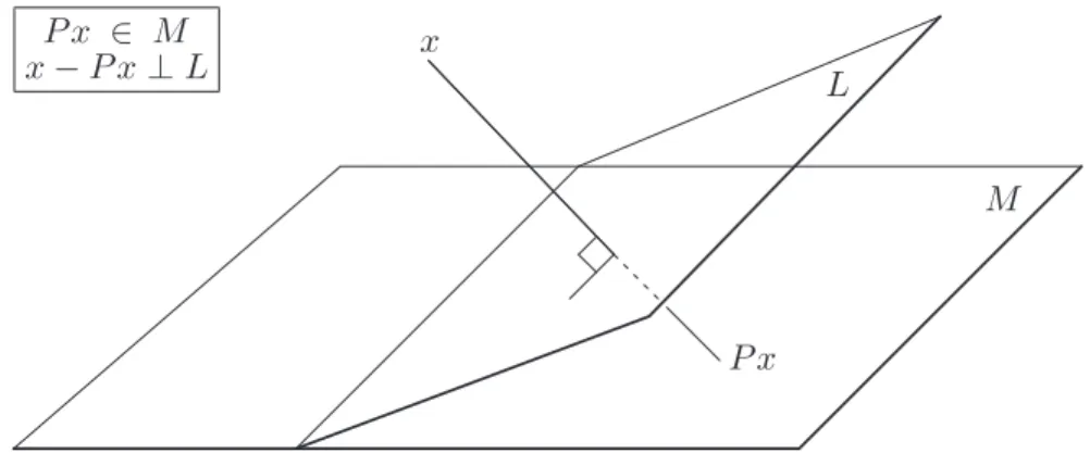
It is orthonormal if, in addition, every vector ofGhas a 2-norm equal to unity. A vector that is orthogonal to all the vectors of a subspaceSis said to be orthogonal to this subspace. The set of all the vectors that are orthogonal toSis a vector subspace called the orthogonal complement ofS and denoted by S⊥. The spaceCn _{is the}

direct sum ofSand its orthogonal complement. Thus, any vectorxcan be written in a unique fashion as the sum of a vector inSand a vector inS⊥_{. The operator which} mapsxinto its component in the subspaceSis the orthogonal projector ontoS.

Every subspace admits an orthonormal basis which is obtained by taking any basis and “orthonormalizing” it. The orthonormalization can be achieved by an al-gorithm known as the Gram-Schmidt process which we now describe.

Given a set of linearly independent vectors{x1, x2, . . . , xr}, first normalize the

vectorx1, which means divide it by its 2-norm, to obtain the scaled vector q1 of norm unity. Thenx2is orthogonalized against the vectorq1by subtracting fromx2 a multiple ofq1to make the resulting vector orthogonal toq1, i.e.,

x2 ←x2−(x2, q1)q1.

The resulting vector is again normalized to yield the second vectorq2. Thei-th step of the Gram-Schmidt process consists of orthogonalizing the vector xi against all

previous vectorsqj.

ALGORITHM1.1 Gram-Schmidt

1. Computer11:=kx1k2. Ifr11= 0Stop, else computeq1 :=x1/r11. 2. Forj= 2, . . . , rDo:

3. Computerij := (xj, qi) , fori= 1,2, . . . , j−1

4. qˆ:=xj −

j−1

P

i=1

rijqi

5. rjj :=kqˆk2,

6. Ifrjj = 0then Stop, elseqj := ˆq/rjj

7. EndDo

It is easy to prove that the above algorithm will not break down, i.e., allr steps will be completed if and only if the set of vectorsx1, x2, . . . , xris linearly

indepen-dent. From lines 4 and 5, it is clear that at every step of the algorithm the following relation holds:

xj = j

X

i=1

(32)

If X = [x1, x2, . . . , xr], Q = [q1, q2, . . . , qr], and if R denotes the r ×r upper

triangular matrix whose nonzero elements are therij defined in the algorithm, then

the above relation can be written as

X=QR. (1.19)

This is called the QR decomposition of then_×rmatrixX. From what was said above, the QR decomposition of a matrix exists whenever the column vectors ofX

form a linearly independent set of vectors.

The above algorithm is the standard Gram-Schmidt process. There are alterna-tive formulations of the algorithm which have better numerical properties. The best known of these is the Modified Gram-Schmidt (MGS) algorithm.

ALGORITHM1.2 Modified Gram-Schmidt

1. Definer11:=kx1k2. Ifr11= 0Stop, elseq1 :=x1/r11. 2. Forj= 2, . . . , rDo:

3. Defineqˆ:=xj

4. Fori= 1, . . . , j₋1, Do: 5. rij := (ˆq, qi)

6. qˆ:= ˆq₋rijqi

7. EndDo

8. Computerjj :=kqˆk2,

9. Ifrjj = 0then Stop, elseqj := ˆq/rjj

10. EndDo

Yet another alternative for orthogonalizing a sequence of vectors is the House-holder algorithm. This technique uses HouseHouse-holder reflectors, i.e., matrices of the form

P =I ₋2wwT, (1.20)

in whichwis a vector of 2-norm unity. Geometrically, the vector P xrepresents a mirror image ofxwith respect to the hyperplanespan{w}⊥_.

To describe the Householder orthogonalization process, the problem can be for-mulated as that of finding a QR factorization of a givenn_×mmatrixX. For any vectorx, the vectorwfor the Householder transformation (1.20) is selected in such a way that

P x=αe1, whereαis a scalar. Writing(I₋2wwT_)x₌_αe

1yields

2wTx w=x−αe1. (1.21)

This shows that the desiredwis a multiple of the vectorx₋αe1,

w=± x−αe1 kx₋αe1k2

.

For (1.21) to be satisfied, we must impose the condition

(33)

1.7. ORTHOGONAL VECTORS AND SUBSPACES 13

which gives 2(kxk2

1 −αξ1) = kxk22 −2αξ1 +α2, where ξ1 ≡ eT1x is the first component of the vectorx. Therefore, it is necessary that

α=±kxk2.

In order to avoid that the resulting vectorwbe small, it is customary to take

α=₋sign(ξ1)kxk2,

which yields

w= x+ sign(ξ1)kxk2e1 kx+ sign(ξ1)kxk2e1k2

. (1.22)

Given ann_×mmatrix, its first column can be transformed to a multiple of the columne1, by premultiplying it by a Householder matrixP1,

X1 ≡P1X, X1e1 =αe1.

Assume, inductively, that the matrixX has been transformed ink₋1 successive steps into the partially upper triangular form

Xk≡Pk−1. . . P1X1 =

            

x11 x12 x13 · · · x1m

x22 x23 · · · x2m

x33 · · · x3m

. .. _{· · ·} _{· · ·} .._.

xkk · · · ...

xk+1,k · · · xk+1,m

..

. ... ...

xn,k · · · xn,m

             .

This matrix is upper triangular up to column number k₋1. To advance by one step, it must be transformed into one which is upper triangular up thek-th column, leaving the previous columns in the same form. To leave the first k−1 columns unchanged, select awvector which has zeros in positions 1throughk₋1. So the next Householder reflector matrix is defined as

Pk=I−2wkwkT, (1.23)

in which the vectorwkis defined as

wk=

z kz_k2

, (1.24)

where the components of the vectorzare given by

zi =

 



0 if i < k β+xii if i=k

xik if i > k

(34)

with

β = sign(xkk)× n

X

i=k

x2_ik !1/2

. (1.26)

We note in passing that the premultiplication of a matrixX by a Householder transform requires only a rank-one update since,

(I −2wwT)X=X−wvT where v= 2XTw.

Therefore, the Householder matrices need not, and should not, be explicitly formed. In addition, the vectorswneed not be explicitly scaled.

Assume now thatm−1Householder transforms have been applied to a certain matrixXof dimensionn_×m, to reduce it into the upper triangular form,

Xm ≡Pm−1Pm−2. . . P1X =

            

x11 x12 x13 · · · x1m

x22 x23 · · · x2m

x33 · · · x3m

. .. .._. xm,m 0 .. . .. .              . (1.27)

Recall that our initial goal was to obtain a QR factorization ofX. We now wish to recover theQandRmatrices from thePk’s and the above matrix. If we denote by

P the product of thePion the left-side of (1.27), then (1.27) becomes

P X =

R O

, (1.28)

in whichR is anm_×m upper triangular matrix, andO is an(n₋m)_×mzero block. SinceP is unitary, its inverse is equal to its transpose and, as a result,

X=PT

R O

=P1P2. . . Pm−1

R O

.

IfEmis the matrix of sizen×mwhich consists of the firstmcolumns of the identity

matrix, then the above equality translates into

X=PTEmR.

The matrixQ=PTEmrepresents themfirst columns ofPT. Since

QTQ=E_mTP PTEm =I,

QandRare the matrices sought. In summary,

(35)

1.8. CANONICAL FORMS OF MATRICES 15

in whichRis the triangular matrix obtained from the Householder reduction of X

(see (1.27) and (1.28)) and

Qej =P1P2. . . Pm−1ej.

ALGORITHM1.3 Householder Orthogonalization

1. DefineX= [x1, . . . , xm]

2. Fork= 1, . . . , mDo:

3. Ifk >1computerk:=Pk−1Pk−2. . . P1xk

4. Computewkusing (1.24), (1.25), (1.26)

5. Computerk :=PkrkwithPk =I−2wkwT_k

6. Computeqk=P1P2. . . Pkek

7. EndDo

Note that line 6 can be omitted since theqiare not needed in the execution of the

next steps. It must be executed only when the matrixQis needed at the completion of the algorithm. Also, the operation in line 5 consists only of zeroing the components

k+ 1, . . . , nand updating thek-th component ofrk. In practice, a work vector can

be used forrkand its nonzero components after this step can be saved into an upper

triangular matrix. Since the components 1 throughkof the vectorwkare zero, the

upper triangular matrixRcan be saved in those zero locations which would otherwise be unused.

1.8 Canonical Forms of Matrices

This section discusses the reduction of square matrices into matrices that have sim-pler forms, such as diagonal, bidiagonal, or triangular. Reduction means a transfor-mation that preserves the eigenvalues of a matrix.

Definition 1.5 Two matricesAandBare said to be similar if there is a nonsingular matrixXsuch that

A=XBX−1.

The mappingB _→Ais called a similarity transformation.

It is clear that similarity is an equivalence relation. Similarity transformations pre-serve the eigenvalues of matrices. An eigenvectoruB ofB is transformed into the

eigenvectoruA =XuBofA. In effect, a similarity transformation amounts to

rep-resenting the matrixBin a different basis. We now introduce some terminology.

1. An eigenvalueλofAhas algebraic multiplicityµ, if it is a root of multiplicity

µof the characteristic polynomial.

(36)

3. The geometric multiplicityγ of an eigenvalueλofAis the maximum number of independent eigenvectors associated with it. In other words, the geometric multiplicityγ is the dimension of the eigenspaceNull (A₋λI).

4. A matrix is derogatory if the geometric multiplicity of at least one of its eigen-values is larger than one.

5. An eigenvalue is semisimple if its algebraic multiplicity is equal to its geomet-ric multiplicity. An eigenvalue that is not semisimple is called defective.

Often, λ1, λ2, . . . , λp (p ≤ n) are used to denote the distinct eigenvalues of

A. It is easy to show that the characteristic polynomials of two similar matrices are identical; see Exercise 9. Therefore, the eigenvalues of two similar matrices are equal and so are their algebraic multiplicities. Moreover, ifvis an eigenvector ofB, then

Xvis an eigenvector ofAand, conversely, ifyis an eigenvector ofAthenX−1yis an eigenvector ofB. As a result the number of independent eigenvectors associated with a given eigenvalue is the same for two similar matrices, i.e., their geometric multiplicity is also the same.

1.8.1 Reduction to the Diagonal Form

The simplest form in which a matrix can be reduced is undoubtedly the diagonal form. Unfortunately, this reduction is not always possible. A matrix that can be reduced to the diagonal form is called diagonalizable. The following theorem char-acterizes such matrices.

Theorem 1.6 A matrix of dimensionnis diagonalizable if and only if it hasn line-arly independent eigenvectors.

Proof. A matrixAis diagonalizable if and only if there exists a nonsingular matrix

X and a diagonal matrixDsuch thatA = XDX−1_{, or equivalently}_AX ₌ _XD_, whereDis a diagonal matrix. This is equivalent to saying thatnlinearly independent vectors exist — thencolumn-vectors ofX— such thatAxi =dixi. Each of these

column-vectors is an eigenvector ofA.

A matrix that is diagonalizable has only semisimple eigenvalues. Conversely, if all the eigenvalues of a matrixAare semisimple, then Ahasneigenvectors. It can be easily shown that these eigenvectors are linearly independent; see Exercise 2. As a result, we have the following proposition.

Proposition 1.7 A matrix is diagonalizable if and only if all its eigenvalues are

semisimple.

(37)

1.8.2 The Jordan Canonical Form

From the theoretical viewpoint, one of the most important canonical forms of ma-trices is the well known Jordan form. A full development of the steps leading to the Jordan form is beyond the scope of this book. Only the main theorem is stated. Details, including the proof, can be found in standard books of linear algebra such as [164]. In the following, mi refers to the algebraic multiplicity of the individual

eigenvalueλiandliis the index of the eigenvalue, i.e., the smallest integer for which

Null(A₋λiI)li+1= Null(A−λiI)li.

Theorem 1.8 Any matrixA can be reduced to a block diagonal matrix consisting ofpdiagonal blocks, each associated with a distinct eigenvalue λi. Each of these

diagonal blocks has itself a block diagonal structure consisting of γi sub-blocks,

whereγiis the geometric multiplicity of the eigenvalueλi. Each of the sub-blocks,

referred to as a Jordan block, is an upper bidiagonal matrix of size not exceeding li ≤ mi, with the constant λi on the diagonal and the constant one on the super

diagonal.

Thei-th diagonal block,i= 1, . . . , p, is known as thei-th Jordan submatrix (some-times “Jordan Box”). The Jordan submatrix numberistarts in columnji ≡ m1 +

m2+· · ·+mi−1+ 1. Thus,

X−1AX=J =          J1 J2 . .. Ji . .. Jp          ,

where eachJiis associated withλiand is of sizemithe algebraic multiplicity ofλi.

It has itself the following structure,

Ji=



  

Ji1

Ji2 . ..

Jiγi



 

 withJik= 

  

λi 1

. .. ...

λi 1

λi



  .

Each of the blocksJik corresponds to a different eigenvector associated with the

eigenvalueλi. Its sizeli is the index ofλi.

1.8.3 The Schur Canonical Form

(38)

Theorem 1.9 For any square matrixA, there exists a unitary matrixQsuch that QHAQ=R

is upper triangular.

Proof. The proof is by induction over the dimension n. The result is trivial for

n = 1. Assume that it is true forn₋1 and consider any matrixAof sizen. The matrix admits at least one eigenvectoruthat is associated with an eigenvalueλ. Also assume without loss of generality that_ku_k2 = 1. First, complete the vectoruinto an orthonormal set, i.e., find ann_×(n₋1)matrixV such that then_×nmatrix

U = [u, V]is unitary. ThenAU = [λu, AV]and hence,

UHAU =

uH VH

[λu, AV] =

λ uHAV 0 VHAV

. (1.29)

Now use the induction hypothesis for the(n₋1)_×(n₋1)matrixB = VHAV: There exists an (n₋1)_×(n₋1)unitary matrix Q1 such thatQH1 BQ1 = R1 is upper triangular. Define then×nmatrix

ˆ Q1 =

1 0 0 Q1

and multiply both members of (1.29) byQˆH₁ from the left andQˆ1from the right. The resulting matrix is clearly upper triangular and this shows that the result is true for

A, withQ= ˆQ1U which is a unitaryn×nmatrix.

A simpler proof that uses the Jordan canonical form and the QR decomposition is the subject of Exercise 7. Since the matrixRis triangular and similar toA, its diagonal elements are equal to the eigenvalues ofAordered in a certain manner. In fact, it is easy to extend the proof of the theorem to show that this factorization can be obtained with any order for the eigenvalues. Despite its simplicity, the above theorem has far-reaching consequences, some of which will be examined in the next section.

It is important to note that for anyk _≤ n, the subspace spanned by the first k

columns ofQis invariant underA. Indeed, the relationAQ =QR implies that for

1≤j≤k, we have

Aqj = i=j

X

i=1

rijqi.

If we letQk = [q1, q2, . . . , qk]and ifRkis the principal leading submatrix of

dimen-sionkofR, the above relation can be rewritten as

AQk =QkRk,

(39)

usually called Schur vectors. Schur vectors are not unique and depend, in particular, on the order chosen for the eigenvalues.

A slight variation on the Schur canonical form is the quasi-Schur form, also called the real Schur form. Here, diagonal blocks of size2×2 are allowed in the upper triangular matrixR. The reason for this is to avoid complex arithmetic when the original matrix is real. A2_×2block is associated with each complex conjugate pair of eigenvalues of the matrix.

Example 1.2. Consider the3_×3matrix

A= 



1 10 0 −1 3 1 −1 0 1



.

The matrixAhas the pair of complex conjugate eigenvalues

2.4069. . ._±i_×3.2110. . .

and the real eigenvalue0.1863. . .. The standard (complex) Schur form is given by the pair of matrices

V = 



0.3381−0.8462i 0.3572−0.1071i 0.1749 0.3193₋0.0105i ₋0.2263₋0.6786i ₋0.6214 0.1824 + 0.1852i ₋0.2659₋0.5277i 0.7637





and

S = 



2.4069 + 3.2110i 4.6073₋4.7030i ₋2.3418₋5.2330i 0 2.4069−3.2110i −2.0251−1.2016i

0 0 0.1863



.

It is possible to avoid complex arithmetic by using the quasi-Schur form which con-sists of the pair of matrices

U = 



−0.9768 0.1236 0.1749 −0.0121 0.7834 ₋0.6214 0.2138 0.6091 0.7637





and

R= 



1.3129 −7.7033 6.0407 1.4938 3.5008 ₋1.3870 0 0 0.1863



.

We conclude this section by pointing out that the Schur and the quasi-Schur forms of a given matrix are in no way unique. In addition to the dependence on the ordering of the eigenvalues, any column ofQcan be multiplied by a complex sign

(40)

1.8.4 Application to Powers of Matrices

The analysis of many numerical techniques is based on understanding the behavior of the successive powersAk_{of a given matrix}_A_{. In this regard, the following theorem}

plays a fundamental role in numerical linear algebra, more particularly in the analysis of iterative methods.

Theorem 1.10 The sequence Ak, k = 0,1, . . . , converges to zero if and only if ρ(A)<1.

Proof. To prove the necessary condition, assume that Ak _→ ₀_{and consider} _u

1 a unit eigenvector associated with an eigenvalueλ1 of maximum modulus. We have

Aku1 =λk1u1,

which implies, by taking the 2-norms of both sides,

|λk₁_|=_kAku1k2 →0.

This shows thatρ(A) =|λ1|<1.

The Jordan canonical form must be used to show the sufficient condition. As-sume thatρ(A)<1. Start with the equality

Ak=XJkX−1.

To prove that Ak converges to zero, it is sufficient to show that Jk converges to zero. An important observation is thatJk_{preserves its block form. Therefore, it is}

sufficient to prove that each of the Jordan blocks converges to zero. Each block is of the form

Ji =λiI+Ei

whereEiis a nilpotent matrix of indexli, i.e.,Eili = 0. Therefore, fork≥li,

J_ik=

li−1

X

j=0

k! j!(k−j)!λ

k−j i E

j i.

Using the triangle inequality for any norm and takingk≥li yields

kJ_ik_{k ≤}

li−1

X

j=0

k!

j!(k−j)!|λi|

k−j_k_Ej ik.

Since |λi| < 1, each of the terms in this finite sum converges to zero as k → ∞.

Therefore, the matrixJ_ikconverges to zero.

(41)

1.9. NORMAL AND HERMITIAN MATRICES 21

Theorem 1.11 The series

∞

X

k=0

Ak

converges if and only ifρ(A) <1. Under this condition, I₋Ais nonsingular and the limit of the series is equal to(I₋A)−1_.

Proof. The first part of the theorem is an immediate consequence of Theorem 1.10. Indeed, if the series converges, then kAkk → 0. By the previous theorem, this implies thatρ(A)<1. To show that the converse is also true, use the equality

I₋Ak+1= (I₋A)(I+A+A2+. . .+Ak)

and exploit the fact that sinceρ(A)<1, thenI−Ais nonsingular, and therefore,

(I₋A)−1(I₋Ak+1) =I+A+A2+. . .+Ak.

This shows that the series converges since the left-hand side will converge to(I − A)−1. In addition, it also shows the second part of the theorem.

Another important consequence of the Jordan canonical form is a result that re-lates the spectral radius of a matrix to its matrix norm.

Theorem 1.12 For any matrix normk._k, we have lim

k→∞kA

k_k1/k ₌_ρ(A).

Proof. The proof is a direct application of the Jordan canonical form and is the subject of Exercise 10.

1.9 Normal and Hermitian Matrices

This section examines specific properties of normal matrices and Hermitian matrices, including some optimality properties related to their spectra. The most common normal matrices that arise in practice are Hermitian or skew-Hermitian.

1.9.1 Normal Matrices

By definition, a matrix is said to be normal if it commutes with its transpose conju-gate, i.e., if it satisfies the relation

AHA=AAH. (1.30)

An immediate property of normal matrices is stated in the following lemma.