Forecasting Stock Markets Using Machine
Learning
André Dinis Oliveira
Forecasting the PSI-20 index using a Machine Learning
approach
Trabalho de Projeto apresentado como requisito parcial para
obtenção do grau de Mestre em Estatística e Gestão de
NOVA Information Management School
Instituto Superior de Estatística e Gestão de Informação Universidade Nova de Lisboa
FORECASTING
STOCK
MARKETS
USING
MACHINE
LEARNING
por
André Dinis Oliveira
Trabalho de Projeto apresentado como requisito parcial para a obtenção do grau de Mestre em Estatística e Gestão de Informação, Especialização em Análise e Gestão de Risco
Orientador: Prof. Mauro Castelli
ACKNOWLEDGEMENTS
It would be hard to do this work project without the help of Prof. Mauro Castelli that gave me full support trough out this adventure. I am sincerely grateful for all the material, discussion and patience provided.
I also wish to thank my friends that were always available to distracted me during the up’s and down’s of my life and this Master project. A special thanks to O Fred.
Por fim quero agradecer `a minha M˜ae persistente , ao meu Pai compreendedor, ao chato do meu irm˜ao Adriano e `a minha querida irm˜a Helena. A vossa ajuda e paciˆencia foi essencial.
ABSTRACT
Predicting financial markets is a task of extreme difficulty. The factors that influence stock prices are extremely complex to model. Machine Learning algorithms have been widely used to predict financial markets with some degree of success. This Master’s project aims to study the application of these algorithms to the Portuguese stock market, the PSI-20, with special emphasis on genetic programming and the introduction of the concept of semantics in the process of evolution. Three systems based on genetic programming were studied: STGP, GSGP and GSGP-LS. The construction of the predictive models is based on historical information of the index extracted through a blooberg portal. In order to analyze the quality of the models based on genetic programming, the final results were compared with other Machine Learning algorithms through the application of significance statistical tests. An analysis of the quality of the results of the different algorithms is presented and discussed.
KEYWORDS
RESUMO
Prever mercados financeiros ´e uma tarefa de extrema dificuldade. Os fatores que influenciam os pre¸cos de ac¸c˜oes s˜ao de natureza complexa e de dif´ıcil modeliza¸c˜ao. Algoritmos baseados em aprendizagem autom´atica tˆem sido bastante utilizados para prever os mercados financeiros com algum grau de sucesso. Este projeto de Mestrado tem o objetivo de estudar a aplica¸c˜ao destes algoritmos ao mercado de ac¸c˜oes portuguˆes, o PSI-20, com especial destaque para a aplica¸c˜ao de programa¸c˜ao gen´etica e para a introdu¸c˜ao do conceito de semˆantica no processo de evolu¸c˜ao. Trˆes sistemas baseados em programa¸c˜ao gen´etica foram estudados: STGP, GSGP and GSGP-LS. A constru¸c˜ao dos modelos preditivos baseia-se em informa¸c˜ao hist´orica do ´ındice extraida atrav´es de um portal blooberg. Para analisar a qualidade dos modelos baseados em programa¸c˜ao gen´etica, os resultados finais foram comparados com outros algoritmos da ´area de aprendizagem autom´atica atrav´es da aplica¸c˜ao de testes de significˆancia estat´ıstica. Uma an´alise `a qualidade dos resultados dos diferentes algoritmos ´e apresentada e discutida.
PALAVRAS-CHAVE
INDEX
1 Introduction 1
1.1 Forecasting Problem . . . 2
1.2 Research Objectives . . . 3
1.3 Document Structure . . . 4
2 Literature Review 5 3 Machine Learning 9 3.1 Introduction . . . 9
3.2 Genetic Programming . . . 10
3.2.1 Representation of Individuals . . . 11
3.2.2 Initialization the Population . . . 12
3.2.3 Fitness Function . . . 15
3.2.4 Selection . . . 15
3.2.5 Genetic Operators . . . 16
3.2.7 Termination Criterion . . . 19
3.3 Geometric Semantic Genetic Programming . . . 20
3.3.1 Local Search in Geometric Semantic Operators . . . 22
3.4 Other ML Teqcnhiques . . . 25
3.4.1 Linear Regression - LR . . . 25
3.4.2 Support Vector Machines - SVM . . . 26
3.4.3 Artificial Neural Networks - ANN . . . 27
4 Methodology 29 4.1 Introduction . . . 29
4.2 Machine Learning Algorithm . . . 31
4.2.1 Software Methodology . . . 32
4.3 Data Description . . . 32
4.3.1 Data Transformation . . . 33
4.4 Experimental settings . . . 34
5 Results and Discussion 36 5.1 Comparison with other ML algorithms . . . 40
6 Conclusion and Future work 42
List of Figures
3.1 General description of GP algorithm . . . 11
3.2 GP Tree-based representation of 10x+ 10 . . . 12
3.3 Two examples of individuals created by full method with maximum depth=2. 3.3a represents the tree syntax forf(x, y) =Sin(x)+(x−y) and 3.3b the tree syntax for f(x, y) = x∗y+x/y . . . 13
3.4 Three examples of individuals created by grow method with depth limit=2. 3.4a represents the tree syntax forf(x, y) = xand 3.4b the tree syntax for f(x, y) = (x+y) + 10 and 3.4c for f(x, y) = x∗y+x/y . . . 14
3.5 Example of subtree crossover . . . 17
3.6 Example of subtree mutation . . . 18
3.7 A visual intuition of a two-dimensional semantic space that is used to explain properties of the geometric semantic crossover presented in Moraglio (2012). . . 22
3.8 A graphical representation of (a) GSM and (b) GSM-LS . . . 23
3.9 Schematic of a single hidden layer neural network . . . 28
4.1 General Machine Learning System . . . 31
5.1 Comparison between the three GP systems: results obtained for the PSI-20 index dataset. Evolution of (a) training and (b) test errors
for each technique (MAE), median over 50 independent runs. . . 36
5.2 Comparison between the three GP systems: results obtained for the PSI-20 index dataset. Evolution of (a) training and (b) test errors
List of Tables
3.1 Three examples of possible primitive set . . . 12
4.1 The Data Set . . . 34
4.2 Experimental Settings . . . 35
5.1 Comparison between the GP systems: reports the median values obtained for the last generation . . . 37
5.2 P-values given by the statistical test for the GP systems . . . 39
5.3 Experimental comparison between different non-evolutionary techniques and GSGP . . . 40
ACRONYMS
ML Machine Learning: is the subfield of computer science that ”gives computers
the ability to learn without being explicitly programmed”
GP Genetic Programming: Evolutionary algorithm that mimics Darwin’s theory
of evolution of species
GSO Geometric Semantic Operators: new genetic operators that incorporate in
the process of evolution the concept of semantics.
SVM Support Vector Machines: algorithm belonging to ML field often used to
solve regression and segmentation problems. Frequency
ANN Artificial Neural Networks: algorithm belonging to ML that is bio-inspired
Chapter 1
Introduction
Stock price time-series are often characterized by a chaotic and non-linear behaviour which makes the forecast a challenging task. The factors that produces uncertainty in this field are complex and from different nature, from economic, political and investment decisions to unclear reasons that, somehow, produce effects and make hard to predict how the prices will evolve. The stock market attracts investments due to the ability of producing high revenues. However, owing to its risky nature, there is a need for an intelligent tool that minimizes risks and, hopefully, maximizes profits.
Predicting stock prices using historical data of the time-series to provide an estimate of future values is the most common approach among the literature. More recently, researchers have started to develop machine learning (ML) techniques that resemble biological and evolutionary process to solve complex and non-linear problems. This work contrasts the typical approach, where classical statistical
methods are employed. Examples of such ML techniques are Artificial Neural
Networks (ANN), Support Vector Machines and Genetic Programming (GP).
Genetic Programming (GP) belongs to the field of evolutionary computation
where algorithms are inspired on Darwin theory of evolution. In GP possible
using genetic operators (crossover and mutation) to produce, hopefully, better individuals. In the first description of GP made by Koza (1992), these genetic operators produce
new individuals simply by changing the syntax of the parents without taking into
account the semantics of the individuals. The concept of semantics in GP usually
refers to the vector of outputs produced by a GP individual on a set of training data. Recently, new gentic operators called geometric semantic operators have been proposed by Moraglio (2012). These operators have the interesting characteristic of inducing an unimodal fitness landscape on any supervised learning problem. However, these operators also presents a serious limitation, they produce individuals that are much larger then their parents which makes the size of the individuals in the population increasing exponentially over the generations.
The objective of this project is the application of genetic programming systems to forecast the PSI-20 index, the Portuguese stock market. The approach proposed in this work is to analyse the performance of different GP systems to predict the next day price.
1.1
Forecasting Problem
The application of ML algorithms, more specifically GP, can be helpful in various financial problems. It has already been applied successfully in financial forecasting, trading strategies optimization and financial modelling.
This Master project focus on forecasting stock prices time-series using a machine learning approach. Considering a short-term forecasting problem
(one-day-head forecast), the objective is to predict the stock price in givendayt+1 using a set
of inputs variables that represents the past stock prices up to dayt. The problem
can be described as follow: given a set of inputs variables,xt, xt−1, ..., xt−m we have:
ˆ
xt+1 = ˆf(xt, xt−1, ..., xt−n) (1.1)
ML algorithms play the role of finding the best forecast function, ˆf, through the identification of hidden patterns and relations in the data either by parameter optimization, creation of expressions and variable selection.
Although this project is applied to forecast financial time-series, it should not be only of value to the financial sector. In general, ML can be used to forecast and modelling any type of time-series.
1.2
Research Objectives
This project aims to apply ML algorithms to one of the most challenging tasks of the financial sector: forecasting financial time-series. Financial agents can benefit from systems based on ML to planning and monitoring their financial investments more accurately and therefore achieving higher returns.
The main goal of this work is the application of Genetic Programming (GP) and some new advances in the field, namely the introduction of geometric semantic operators, to the problem of finding the best model that, given historical data, can predict the price of the stock in the future.
In order to achieve the main goal, the following specific steps are set:
• A description of the ML algorithms with special emphasis in the field of GP
and its use in the financial sector.
• Selection of a financial time-series to develop the experimental work.
• Description of the data and the methodology used.
• Assessment of the performance of the models produced by the considered GP
systems:
– Geometric Semantic Genetic Programming (GSGP)
– Geometric Semantic Genetic Programming with Local Search
(GSGP-LS).
• A comparison of the performance of the models between different ML approaches
1.3
Document Structure
The paragraphs bellow describes how the rest of the document is structured.
Chapter 2, Literature Review, summarizes the past work done on this field. The main topics analysed in the scope of this project are Genetic Programming and Machine Learning approaches to forecast the financial markets.
Chapter 3, Genetic Programming, presents mainly an overview of GP, some advances made recently in the field, such the introduction of the concept of ”semantics” in GP and a brief description of other ML algorithms used in this field.
Chapter 4, Methodology and Data, describes the approach implemented during this project to design a forecast system based on GP, the dataset, the preparation and preprocessing of the data.
Chapter 5, Results and Discussion, presents the outcome of the project and a interpretation of the results provided.
Chapter 2
Literature Review
This chapter presents the literature and previous activities that are most relevant for this work project. The literature review is done accordantly with the most relevant subjects that were taking into account for the preparation of this project, more specifically, Genetic Programming and Machine Learning techniques to forecast stock prices.
Machine learning algorithms have been widely applied in many areas of finance. More specifically, ML techniques are common accepted to predict stock markets by means of a regression or classification problems. Usually, we have a quantitative output measurement (such as a stock price) or categorical (such as stock price goes up/down), that we wish to predict based on a set of variables, for example the stock prices of previous days or other indicators that could explain the final outcome. The use of ML algorithms allows us to build predictive models that can explain the relation between input and output variables on an set of training data.
Considering an Supervised Learning approach, the agent is provided with known
Some relevant articles about using ML techniques to predict the stock markets are listed here.Atsalakis & Valavanis (2009) presents a survey on neural and neuro-fuzzy techniques to forecast stock markets. It is shown that these techniques are widely accepted to studying and performing stock market prediction. Shen
et al. (2012) proposes a prediction algorithm that exploits the use of temporal correlation among global stock markets and various financial products to predict the next-day stock trend using SVM. The author performs an empirical study on NASDAQ, S&P500 and DJIA indexes achieving good results. Choudhry & Garg (2008) investigate the use of an hybrid machine learning system based on Genetic Algorithm (GA) and Support Vector Machines (SVM) for stock market forecasting. The genetic algorithm is used to choose the set of most informative input variables from the entire dataset. The results showed that the hybrid GA-SVM system outperforms the stand alone SVM system.
There are numerous papers exploiting the use of Genetic Programming to forecast stock prices. For instance, Hui (2003) presents a standard GP approach to forecast the IBM stock prices. The paper presents an experimental study, which aims to analyze how the GP parameters (population size, number of generations,
etc) effects the final accurracy of the GP model. Sheta et al. (2013) developed a
intelligent application based on GP was developed to forecast financial markets which allowed the authors to win the competition organized within the CEC2000 on ”Dow Jones Prediction”. Lee & Tong (2011) proposes a hybrid forecasting model for nonlinear time series by considering both ARIMA and GP models to improve upon both the ANN and the ARIMA forecasting models. The results indicate improvements in the accuracy of the proposed model against other ML approaches, such ANN and standard GP, both on training and testing instances.
More recently, researchs have been focused on developing new variants of GP to improve its performance. Moraglio (2012) proposes the use of geometric semantic operators which enables the GP system to evolve and improve based on the semantics of the solutions. The concept of semantics in GP is often intended as the vector of outputs produced by a GP program on the training data. Although these new operators have the interesting property of inducing a unimodal fitness landscape, they also have the serious limitation of producing individuals much larger than their parents which makes the size of the individuals in the population increasing exponentially with generations and, making impossible to use them in real life applications.
To surpass this limitation, L. Vanneschi (2013) proposed an efficient implementation of geometric semantic operators (GSGP) which makes possible to use them in real
life applications. In Castelli & Vanneschi (2015) a detailed description of the
Chapter 3
Machine Learning
3.1
Introduction
The use of machine learning techniques in the financial markets, specifically for predicting financial time-series, have been quite successful. Nowadays, researchers and companies are trying to develop intelligent algorithms that can capture the hidden patterns inherent to stock markets in order to predict more efficiently the behaviour of the stock prices. This field falls into the scope of machine learning and predictive models.
In general, the approaches used by researchers can be divided into two main classes:
• The econometric models developed based on statistical approaches such the
Linear Regression (LR), Autoregression Moving Average and ARIMA models. However this models models offer a simple implementation they have the nonrealistic assumption that the financial time-series data follows a linear pattern and is stationary.
• Predictive models for forecasting market stock prices based on intelligent
problems . Examples of such algorithms are Genetic Programming (GP), Artificial Neural Networks (ANN) and Support Vector Machines (SVM).
In the following sections will be presented the most common machine learning algorithms used to predict the stock market, with special emphasis on the Genetic Programming model.
3.2
Genetic Programming
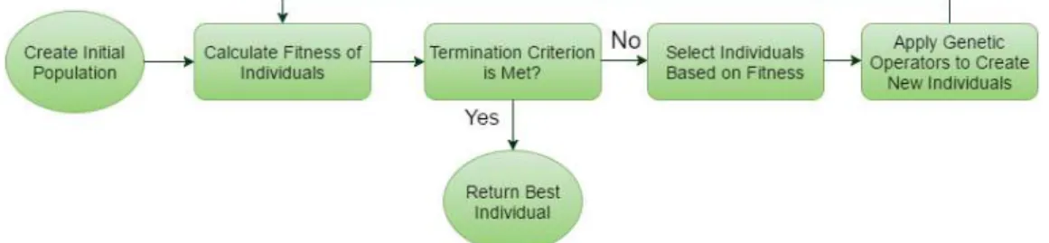
GP represents one of the famous evolutionary computation techniques which seeks to solve wide domain problems automatically. It was first described by Koza (1992) as an automatic and domain-independent method which can create computer programs capable of solving a large variety of problems. Moreover, GP attempts to perform automated learning of computers programs by mimicking the process of Darwinian evolution. In GP the process starts by randomly creating a initial population of computer programs and with generations GP algorithm transforms the population of programs into a new, hopefully better, population of programs through the use of genetic operators, usually mutation and crossover. The quality of the computer programs to solve the specific domain problem is asses by the usage of an appropriate fitness function. A general description of the GP algorithm is described in Figure 3.1. Hence, in order to set up the GP run, there are 4 preparatory steps for solving a given problem with GP:
1. Define the representation space. This means choosing the appropriateTerminal
set and Function Set, together they define the structure that is available for GP to generate the computer programs (individuals).
2. Define thefitness function. Choose an indicate fitness function to evaluate the
candidate solutions.
parameters need to be set (population size, generations, probabilities of applying the genetic operators, etc).
4. Define thetermination criterion. Choose what triggers the GP run to terminate.
Figure 3.1: General description of GP algorithm
3.2.1
Representation of Individuals
In GP it is usual to represent the computer programs or individuals in a tree-based notation (Koza, 1992). The syntax trees are constructed from a set of functions and
terminals, the Function Set and Terminal Set respectively. Together they form the
primitive set of the problem. The primitive set defines the search space which GP will scan, that is, all the individuals that can be generate by the combination of primitives in all possible ways.
The Function Set represents the internal nodes of the trees and in a simple numeric problem the function set could consist, for instance, on the arithmetic functions (+,-,*,/). The Terminal Set may consist of external input variables (e.g x,y,z), function with no arguments (e.g rand() which returns random numbers) and constants. The elements in the Function Set and Terminal Set are specified with
a number of arguments (which is usually called Arity). Table 3.1 presents three
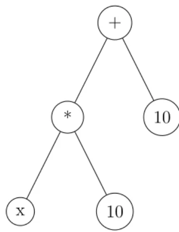
different examples of primitive sets which will be used as examples. For instance, considering the primitive set 1 in table 3.1, Figure 3.2 shows a tree-based syntax
representation of the candidate expression 10x+ 10.
+
*
x 10
10
Figure 3.2: GP Tree-based representation of 10x+ 10
Table 3.1: Three examples of possible primitive set
Primitive Set Function Set Arity Terminal Set Arity
1 (+,-,*,/) (2,2,2,2) (x,y,10) (0,0,0)
2 (+,-,*,/,sin,cos) (2,2,2,2,1,1) (x,y,rand(),10) (0,0,0,0)
3 (AND, OR, NOT) (2,2,1) (x,y) (0,0)
properties known as closure and sufficiency. Sufficiency means that is possible to
create the solution to the problem using the elements available in the primitive set. Unfortunately, ensure that the primitive set is sufficient may not be a easy task. Having a insufficient primitive set, GP can only create programs that approximate the desired one.
The primitive set also needs to ensure the closure property, that is, the function set must be well define for any possible combination of expression that may occur in the process of evolution. For example, considering the tree expression in Fig 3.3b, the / function must be protected for the case when y equals zero. To ensure the closure property for the divide operator, Koza (1992) introduced the protected division, which returns 1 when the denominator equals zero.
3.2.2
Initialization the Population
population are usually randomly created. In GP there are three usual methods of initialization:
• The full method
• The grow method
• The ramped half-and-half method
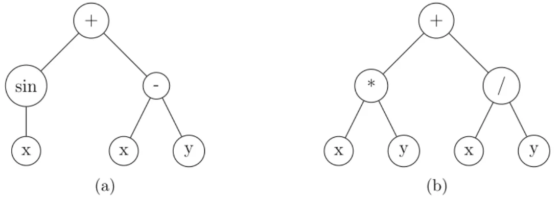
In the full method the initial individuals are created having a pre-specified maximum depth. It is, randomly, selected functions from the Function Set to all nodes of the tree until the maximum tree depth is reached. For the maximum depth level of the tree only terminals can be selected. The full method creates trees which all the leaves (terminals) have the same depth, although this does not mean that all the trees will have the same number of nodes or the same shapes. This only happens if all the functions in the primitive set have equal arity (R. Poli & McPhee., 2008). For example, Figure 3.3 shows two individuals created by the full method with a maximum tree depth equal 2. Although this method will generate all individuals with maximum depth, the shapes may vary depending on the arity of the functions.
Individual 3.3a has a slightly different shape than 3.3b because the sin function
have arity equal to 1 and all functions of 3.3b have arity equal to 2. This method creates all the individuals in the initial population with maximum depth which will diminish the population diversity, at least in the initial population.
+ sin x -x y (a) + * x y / x y (b)
Figure 3.3: Two examples of individuals created by full method with maximum
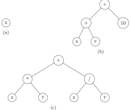
The grow method allows the creation of trees with different sizes and shapes. In this method, nodes are selected from the function and terminal sets until the maximum tree depth is reached. Then, when the maximum depth is reached only terminals can be selected. This method allows to generate individuals with different levels of depth, up to maximum depth. Figure 3.4 shows three individuals created by grow method. Considering the primative set 2 in table 3.1 and with a depth limit equal 2, in 3.4a the node chosen, x, belongs to the terminal set. This prevents the tree of growing any more creating a tree with depth equal 0.
x (a)
+
+
x y
10
(b)
+
*
x y
/
x y
(c)
Figure 3.4: Three examples of individuals created by grow method with depth limit=2.
3.4a represents the tree syntax forf(x, y) = xand 3.4b the tree syntax for f(x, y) =
(x+y) + 10 and 3.4c for f(x, y) =x∗y+x/y
3.2.3
Fitness Function
After determinate the search space, we need to define a measure of performance to quantify how good a candidate solution is. This is done by the definition of a fitness function. The fitness function is the mechanism that tells GP which candidate
solutions or regions of the search space are good. In problems such symbolic
regression, the fitness is usually based on error measures. Two error measures which are widely used for regression problems are, for example, the MAE (Mean Absolute Error) and the RMSE (Root Mean Squared Error) given by the formulas:
M AE = 1
n
n
X
i=1
|fi−yi| (3.1)
RM SE = 1
n v u u t n X i=1
(fi−yi)2 (3.2)
The fitness function evaluates the candidate solution by the amount of error between its output and the desired output.
3.2.4
Selection
In GP genetic operators are applied to individuals that are selected based on fitness, which means that better individuals are more likely to be chosen to be copy to the next population or selected to perform crossover or mutation. The most usual
employed selection methods used in GP are: tournament selection and the fitness
proportionate selection.
selection pressure, (big tournament size), highly benefits the more fit individuals, while a tournament with a weak selection pressure, (small tournament size) gives a better change for less fit individuals to be chosen as parents.
In a fitness proportionate selection, individuals are chosen based on a probability given by:
pi =
fi n
P
i=1 fi
(3.3)
where pi is the probability of individual i to be selected and fi is the fitness of
individuali. This method ensures that better individuals will always be more likely
to be selected as parents for the next population.
3.2.5
Genetic Operators
GP uses genetic operators to create new individuals which will be breed into the new
population. Therefore, the most commonly used operators in GP are the crossover
andmutation operators. The selection of which genetic operators should be used to create new individuals is probabilistic. Their probability of application are called operator rates. Usually, crossover operator is chosen with higher probability and, on
the contrary, mutation operator is less likely to be applied. The crossover rate (pc)
is normally above 90% and the mutation rate (pm) is usually much smaller, typically
being in the region of 1%. When the sum of crossover and mutation rates is less
than 100% a new operator calledreproduction is used with a rate of 100%-(pc+pm).
Crossover Operator
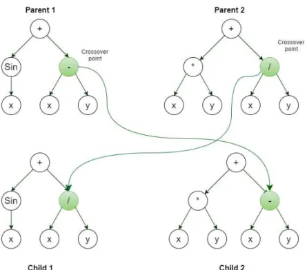
The crossover operators produce new individuals (child’s) by mixing the structure of their parents. The parents are chosen by a selection algorithm introduced in section 3.4. The most commonly used form of crossover is subtree crossover (Koza, 1992), which works in the following way:
2. Select a random subtree from each parent and the root of each subtree is the
crossover point.
3. Create two new individuals (child’s) by swapping the subtrees selected in their parents.
Figure 3.5 shows a example of subtree crossover.
Figure 3.5: Example of subtree crossover
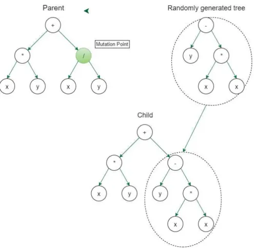
Mutation Operator
Other genetic operator used in GP to change the syntax structure of the trees is the
Mutation operator. The most commonly used form of mutation in GP is the subtree mutation which selects, randomly, a node in the tree and replaces that subtree selected by a random generated tree.
Another common method of mutation used in GP ispoint mutation. When
Figure 3.6: Example of subtree mutation
certain probability is altered by another primitive on the primitive set as explained above. This method allows multiple nodes to be mutated in a single application of point mutation.
Reproduction Operator
The reproduction operator simply involves the copy of the selected individual to the next generation without any modification. Reproduction is often associated with elitism. Elitism consist in copying the best individual, or a percentage of the fittest individuals, of the generation to the next one, without any modification.
3.2.6
GP Parameters
GP to solve the problem. Before any GP run, the user must specify the following parameters:
• Population Size. The population size is an important parameter and its value depends on the complexity of the problem. However, generally GP performs better if the population size is ’bigger’.
• Number of Generations. This parameters indicate the maximum number of generations available for GP to evolve.
• Probabilities of performing the genetic operators. Traditionally, Crossover is applied with a ’big’ probability, usually 90%, and mutation is applied with a ’smaller’ probability, usually less than 5%.
• The Selection method. The most common selection method used in GP is the tournament selection. When using this method, it is also needed to specify another parameter which is the tournament size.
• Population initialization. In many GP applications, it is common generate the initial population using ramped half-half with a depth range of 2-6. This method is more commonly used because it provides a diverse initial population.
3.2.7
Termination Criterion
3.3
Geometric Semantic Genetic Programming
In the earlier sections GP was presented has in Koza (1992). Genetic operators as described above only produces new offspring’s by manipulating their syntactic representation. Although this property allows genetic operators to remain simple and generic search operators it becomes difficult to understand how a modification of the syntax may affect the quality of the individual.
A recent trend in Genetic Programming is the attempt to construct genetic operators that can take into account the semantics of the solution. The concept of semantics in GP is often intend to mean a vector of output values obtained by a set of input data. In order words, the semantics of a solution refers to the behaviour of itself. Regarding on this definition, Moraglio (2012) have introduced geometric
semantic operators for GP:Geometric Semantic Crossover and Geometric Semantic
Mutation. In Moraglio (2012) is presented the formal definitions of this genetic operators.
Definition 3.3.1. Geometric Semantic Crossover(GSC).
Given two parent functions T1,T2 : Rn → R , the geometric semantic crossover
returns the real function TXO = (T1∗TR) + ((1−TR)∗T2), where TR is a random
real function whose output values range in the interval [0,1].
Moraglio (2012) formally proves that this GSC operator corresponds to geometric crossover on the semantic space, and thus induces a unimodal fitness
landscape. In order to TRproduces values in the range of [0, 1] it is usually use the
sigmoid function:
TR=
1
1 +e(−TRand) (3.4)
where TRand is a generated random tree with no constrains.
Definition 3.3.2. Geometric Semantic Mutation(GSM).
Given a parent function T :Rn→R, the geometric semantic mutation with mutation step ms returns the real function TM = T +ms∗(TR1−TR2), where TR1 and TR2
Moraglio (2012) proves that this operator corresponds to ball mutation on the semantic space and induces a unimodal fitness landscape. The random generated
tress TR1 and TR2 have been limited to assume values in the range of [0,1], using
the exact same method describe for TR used in GSC. The parameter ms allows a
’small’ perturbation in the individual because in centred in zero (difference between the two random trees). Despite that, this parameter can be tuned to define a bigger or smaller magnitude of the perturbation produced by this operator.
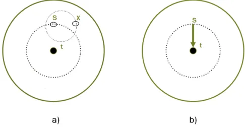
The use of this new genetic operators allows us to produce modifications on the syntactic space of GP individuals that have a exact effect on their semantics. For any supervised learning problem, where the expected output values are known and the fitness consists on the distance in the semantic space between any individual and the target point, these operators have a very interesting property of inducing a uni-modal fitness landscape (error surface), such like regression and classification problems. Other interesting property derived from the definition of this operators is that geometric properties remains independently from the data on which individuals are evaluated. In other words, geometric semantic crossover produces an offspring that lies between the parents also in the semantic space induced by the test data. This is extermely interesting because this operators can be considered a tool to help
control and limitoverffing, offering a satisfatory generalization ability in the test set
(out-of sample data). This last property was first clearly presented in L. Vanneschi (2013) trough the application of this operators to several real life applications.
Figure 3.7: A visual intuition of a two-dimensional semantic space that is used to explain properties of the geometric semantic crossover presented in Moraglio (2012).
Although this operators have the interesting properties explained above, they also have the strong limitation, by construction, of generating offspring’s that are much larger than their parents, provoking an exponential growth in the size of the individuals. In a few generations the size of the individuals in the population becomes incredibly large which makes these operators unusable in real life applications
To overcome this limitation, in L. Vanneschi (2013) is defined a new implementation of these operators, which allows us to use them efficiently. For a more comprehensive
description of this efficient implementation the interested reader in pointed to L. Vanneschi
(2013) and Castelli et al. (2014).
3.3.1
Local Search in Geometric Semantic Operators
TM =α0+α1 ∗T +α2∗(TR1−TR2) (3.5)
where αi ∈ R; notice that α2 replaces the mutation step parameter ms of
the geometric semantic mutation (GSM). The LS operator attempts to determine the best linear combination between the parent tree and the random trees used to perturb it, which is local in the sense of the linear problem posed by the GSM operator. This strategy can be seen as fitting a linear regression model on the GSM operator to improve
It should not be seen as a LS in the entire semantic space, since in that case the LS would necessarily converge thorough to the desired program in the unimodal landscape.
With a local search method integrated, the search process will become more efficient and will improve the convergence speed of the algorithm in order to obtain better performance with respect to the algorithm that only uses the geometric semantic operators. Moreover, by speeding up the search process, it will be possible to limit the construction of over-specialised solutions that could overfit the data.
Figure 3.8: A graphical representation of (a) GSM and (b) GSM-LS
3.4
Other ML Teqcnhiques
In the following subsections will be presented a brief description of other machine learning techniques that are commonly used to perform stock market prediction, such linear regression models, support vector machines and artificial neural networks.
3.4.1
Linear Regression - LR
The linear model has been present for a long time now and remains one of the most important tools in the statistics field. A linear regression model can be represented by the following mathematical expression:
X = (X1, X2, ..., Xp) (3.6a)
β= (β1, β2, ..., βp) (3.6b)
ˆ
Y = ˆβ0+
p
X
j=1
Xjβˆj (3.6c)
whereXi represents the model input variables and Y is the model output variable.
The βi, i=1,2,...,p are the model parameters which need to be estimated.
The term β0 is the intercept, also known as the bias in machine learning.
Often it is convenient to include the constant variable 1 in X, include β0 in the
vector of coefficients β, and then write the linear model in vector form as an inner
product:
ˆ
Y =XTβˆ (3.7)
For the estimation of the coefficients of the model β the most common
approach is to estimate using the least squares method. In this approach β is
estimate in order to minimize the residual sum of squares:
RSS(β) =
N
X
j=1
writing the formula in matrix notation we have:
RSS(β) = (y−Xβ)T(y−Xβ) (3.9)
where X is an N * p matrix with each row an input vector, and y is an N-vector of
the outputs in the training set. Differentiating in order of β and equal to zero we
get the equations:
XT(y−Xβ) = 0 (3.10a)
ˆ
β = (XTX)−1XTy (3.10b)
3.4.2
Support Vector Machines - SVM
Suppport vector machine (SVM) have been implemented in many types of problems such classification, recognition and regression. It was firstly on classification problems, principle to develop binary classifications. The goal of support vector machine is to build a hyperplane as the decision surface such the margin of separation between labels is maximized.
For SVM regression, the inputs X are first mapped into a m-dimensional
feature space using some nonlinear relation, and then a linear model is constructed in this feature space. Using mathematical notation, the linear model is given by
f(X, φ) =
m
X
j=1
(φj∗gj(X)) +b (3.11)
wheregj(X),j=1,...mis the function representing the nonlinear transformations
and b is the ’bias’ term. In order to estimate the quality of the produced outputs is used a loss function proposed by Vapnik.
Lε(y, f(X, φ)) =
0, if |y−f(X, φ)|<=ε
For a more comprehensive explanation of SVM, the reader is referred to the Bibliography (Zhang (2001) and Smola & Sch¨olkopf (2004)).
3.4.3
Artificial Neural Networks - ANN
Artificial neural networks (ANNs) are a bio-inspired computational model that tries to mimic, at some rudimentary level, the behaviour of the human brain. These models are used to estimate or approximate functions by building a system of interconnected ’neurons’ which can compute values from input variables and fit a function the approximate the desired output. The artificial neural networks are
usually presented by having three layers, the input layer which are compose by
the input variables used to modelling the problem, the hidden layer that receive
values from the input layer and provides them for the output layer. All the layers
are connected between each other by correspondingweights to neurons of different
layers. Them, each network is trained through receiving some examples (many pairs of input and outputs) and as a result, weights among layers will change and update by comparing the output of the network with the desired target until the computed values from the networks ’match’ the desired target.
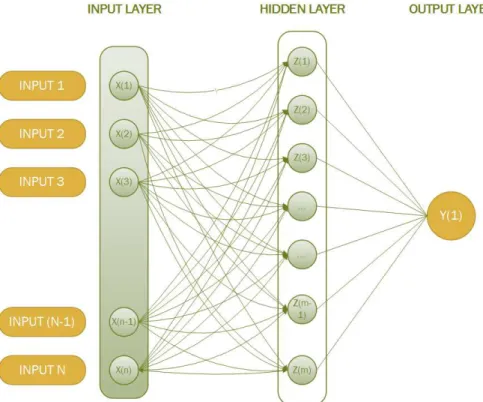
A neural network can be seen as a two-stage regression or classification model, typically represented by a network diagram as in Figure 3.9.
In real life applications, a neural networks is often constructed having more than one hidden layers. A multi layer perceptron (MLP) is a feed forward artificial neural network model that maps sets of input data on to a set of appropriate outputs. A MLP consists of multiple layers of nodes with each layer fully connected to the next one. Except for the input nodes, each node is a neuron (or processing element) with a non-linear activation function.
Figure 3.9: Schematic of a single hidden layer neural network
although tends to converge slowly. To produce a non-linearly relationship between
the layers is necessary to use a nonlinear activation function suchsigmoid function:
φ(s) = 1
1 +e−s (3.12)
Chapter 4
Methodology
4.1
Introduction
Forecasting stock prices can be a challenging task. The process of determining which indicators and input data will be used, and gathering enough training data to training the system appropriately is not obvious. The input data may be raw data on volume, price, or daily change, but also it may include derived data such as technical indicators (moving average, trend-line indicators, etc.) or fundamental indicators (intrinsic share value, economic environment, etc.). It is crucial to understand what data can be useful to capture the underlying patterns and integrate into the machine learning system.
The methodology used in this work consists on applying Machine Learning systems, with special emphasis on Genetic Programming. GP has been considered one of the most successful existing computational intelligence methods and capable to obtain competitive results on a very large set of real-life application against other methods. The experimental work is focused on applying the standard GP, such as the introduction of geometric semantic operators, to forecast the PSI-20 index using historical data and considering one day ahead forecasting.
4.2
Machine Learning Algorithm
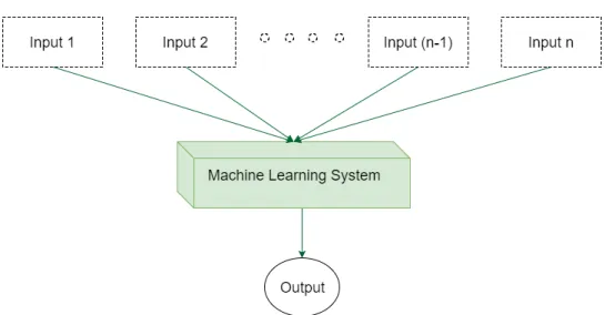
In the chosen approach to predict the next day price of PSI-20 index, it was used a supervised learning approach where the input variables of the algorithm are a set of economic indicators, directly related with the PSI-20 Index, with known time-stamp t. The goal of the Machine Learning System is to use the input variables to predict the values of the outputs.
Figure 4.1 shows how a supervised learning system functions.
Figure 4.1: General Machine Learning System
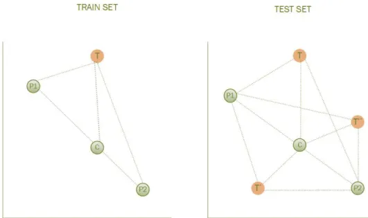
The whole time series, PSI-20 Index prices from 2 January 2014 to 6 May 2016, were divided into the training and the testing data sets as described in Figure 4.2. For the training set was considered the data from 2 January 2014 to 31 December 2015 (500 data observations) and for the testing set the remaining period.
The objective is to predict the stock price at the end of the day t+1
4.2.1
Software Methodology
For the Standard Genetic Programming Application (STGP), a c++ library written for the purpose of this work was implemented.
Regarding the Geometric Semantic Genetic Programming (GSGP) it was used the GSGP implementation freely available at http://gsgp.sourceforge.net and very well documented in Castelli & Vanneschi (2015). GSGP is free/open source c++ library and it provides a robust and efficient implementation of geometric semantic genetic operators for Genetic Programming. This library implements the standard GP algorithm but the genetic operators have embedded the concept of the semantic awareness as explained in section 3.3. It is easily adaptable and its implementation is straightforward, depending on set of configuration parameters.
For the GSGP-LS implementation the same library was used with small adaptations of the source code to include a local search optimizer in the GSM operator.
All the results concerning other Machine Learning Techniques were obtained by using WEKA software.
4.3
Data Description
The data for this work are a set of variables related with the PSI-20 Index from 2 January 2014 to 6 May 2016, which corresponds to 600 data observations. The variables represent historical data relative to the index, namely daily close prices, open price, high price and low price. In Table 4.1 is the description of the dataset used that was transformed using this variables.
Figure 4.2: Evolution of PSI-20 Index close prices (02/01/2014 to 06/05/2016)
4.3.1
Data Transformation
After running a few experiments on raw stock prices the GP systems often reach to a local optimal in a small number generations by predicting a solution similar to last day price. To overcome this problem rather than using raw stock prices, daily
changes in stock prices were used. A new variable xi is defined, which represents
the daily change in price of the time series data:
xi =Pi−Pi−1 (4.1)
This method of differencing the data is commonly used to transform non-stationary time series into non-stationary ones. Given that stock prices are likely to be near with each other considering consecutive days, GP systems will be more likely to produce a solution that resembles on last day price data as output prediction. When
considering daily changes in stock prices the later is not likely to happen because
Table 4.1: The Data Set
Variable Description
(x1,...x10) Daily changes of close prices between consecutive days
x11 The change of open price between consecutive days
x12 The change of high price between consecutive days
x13 The change of low price between consecutive days
x14 The percent change of close prices between consecutive days
Target The change of close price in the next day
4.4
Experimental settings
Three different GP systems were implemented: the standard GP approach (ST-GP), as proposed by Koza (1992); GSGP that uses geometric semantic operators, both
GSC (Geometric Semantic Crossover) and GSM (Geometric Semantic Mutation);
and GSGP with a Local Search Optimizer implemented on the GSM operator, GSGP-LS.
All the systems were set with a population size of 200 individuals evolved for 1000 generations with a total of 50 runs. To perform the tree initialization the Ramped Half-and-Half method was used with a maximum initial depth equal to 6. Selection was made by the tournament selection method with a tournament size of 10. For the STGP, the function set consisted on the arithmetic operators, (+,-,*,/) as well as the cosine, sine, and log functions. For the others GP systems the function set contained only the arithmetic operators. The terminal set consisted of by 14 variables, summarized in Table 4.2. For all systems, Crossover has been used with probability 70% and Mutation with probability 30%. With respect to of GSM
the mutation step was set randomly in each mutation event as in Vanneschi et al.
GP systems, defined as follow:
M AE = 1
n
n
X
i=1
|fi−yi| (4.2)
where fi is the output measure of the GP program and yi is the target value for the
instance i. All the parameters of the systems studied are summarized in Table 4.2.
In the next chapter the results obtained are reported. The experimental results are evaluated by reporting the median error of the training and test sets. For each run, the best individual of the generation is stored and then the median value per generation is reported.
Table 4.2: Experimental Settings
Method
Parameters STGP GSGP GSGP-LS
Terminal set x1,...,x14 x1,...,x14 x1,...,x14
Funcion set +,-,*,/,cos ,sin,log +,-,*,/ +,-,*,/
Fitness Function MAE MAE MAE
Population 200 200 200
Generations 1000 1000 1000
Probability Crossover 0.7 0.7 0.7
Probability Mutation 0.3 0.3 0.3
Elitism best individual best individual best individual
Tournament Size 10 10 10
Max depth creation 6 6 6
Chapter 5
Results and Discussion
The results presented in this section were obtained using the described methodology in subsection 4.2.1. For all the GP systems, 50 runs have been performed. Figure 5.1 reports, for the dataset taken into account, training and test error (MAE) for the all the GP systems considered against generations.
(a) (b)
Figure 5.1: Comparison between the three GP systems: results obtained for the
PSI-20 index dataset. Evolution of (a) training and (b) test errors for each technique (MAE), median over 50 independent runs.
over the mean in reported plots because of its higher robustness to outliers.
Considering STGP and GSGP, Figure 5.1 clearly show that GSGP outperforms STGP on both training and test sets. It is possible to see that GSGP performs well against STGP because the properties of the genetic operators defined in GSGP allow a faster convergence on the training data and it is also possible to note on the testing set that GSGP is able to control overfitting. Although the GSGP in the final generation is able to converge to a lower training error than STGP, on unseen (test) data the two GP systems achieve a comparable test error. Regarding the GSGP-LS system performance, it shows a even faster convergence on the training data with respect to the GSGP system on the first 10 generations. After that, the LS optimizer stops and the performance become like a normal GSGP system. It is possible to note that the application of the LS optimizer despite of producing a faster convergence in the training data also produces a overfit on the testing data, even greater than STGP for the considered dataset. The median results of 50 runs for the last generation are shown in Table 5.1.
Table 5.1: Comparison between the GP systems: reports the median values obtained
for the last generation
Mean Absolute Error
Method Train Test
STGP 61.13 60.02
GSGP 43.28 59.49
GSGP-LS 39.1 62.02
(a) Train (b) Test
Figure 5.2: Comparison between the three GP systems: results obtained for the
PSI-20 index dataset. Evolution of (a) training and (b) test errors for each technique, median over 50 independent runs.
the data achieving test error greater than 100.
In order to study the statistical significance of the final results, at generation
1000, it was firstly used the Shapiro Wilk test, with α=0.05, to test if the data are
normally distributed. The Shapiro Wilk test is based on the following statistic:
W = b
2
n
P
i=1
(x(i)−x¯)
(5.1)
where x(i)are the ordered values,x(1) < x(2) < ... < x(n). The variable b is calculated
in the following way:
b = n/2 X i=1
an−i+1×(x(n−i+1)−x(i)) if n is even
(n+1)/2
X
i=1
an−i+1×(x(n−i+1)−x(i)) if n is odd
(5.2)
where an−i+1 are calculated based on statistical moments from a normal distribution.
rank-sum test, with α = 0.05, was used under the null hypothesis that the samples have equal medians. For a more comprehensive explanation of statistical test performed in this work, the reader is referred to Bibliography Kanji (2006). The p-values obtained are reported in Table 5.2.
Table 5.2: P-values given by the statistical test for the GP systems
STGP GSGP GSGP-LS
Method Train Test Train Test Train Test
STGP - - <0.001 0.0358 <0.001 <0.001
GSGP - - - - <0.001 <0.001
According the p-values, it is possible to say that GSGP produces solutions that are significantly better (i.e., with lower error) than STGP both on training and test data. When comparing the STGP against GSGP-LS, the latter clearly produce significantly better solutions but only on the training set, due to some overfitting in early generations of GSGP-LS, the former ended up producing better results on the test set. Analysing the p-values obtained for the comparison between GSGP and GSGP-LS it is possible to state that GSGP-LS only produces significantly better solutions on the training data, when considering the test data GSGP-LS ended up producing significantly worst solutions. This results were somehow expected in the training data due to how the genetic operators are constructed on the different GP systems. In the testing data the application of the LS optimizer was not beneficial for the PSI-20 dataset. Despite the fact that GSGP-LS is able to achieve an incredible faster convergence in fewer generations, in this case it also ended up producing over-specialized solutions.
5.1
Comparison with other ML algorithms
After comparing the GP systems against each other it is also important to compare against other state-of-the-art ML algorithms, to understand and evaluate the how the results obtained by GP are competitive against more common approaches.
Table 5.3 reports the values of the training and test errors (MAE) of the solutions obtained by all the studied techniques including the GP systems.
Table 5.3: Experimental comparison between different non-evolutionary techniques
and GSGP
Mean Absolute Error
Method Train Test
Linear Regression 63.01 58.6
Isotonic Regression 62.69 57.71
Neural Nets 53.14 71.88
SVM (degree 1) 62.49 58.9
SVM (degree 2) 57.38 66.88
SVM (degree 3) 48.04 76.56
STGP 61.13 60.02
GSGP 43.28 59.49
GSGP-LS 39.1 62.02
From these results, it is possible to say that GSGP and GSGP-LS perform better than all the other methods on training set. Considering both training and test set it is also interesting to note that GSGP and GSGP-LS outperforms well known ML algorithms such as Neural Networks and SVM polynomial degree 2 and 3 for this dataset. For the other cases it is possible to notice that the GP systems is able to produce very comparable results against the other methods
Table 5.4: P-values given by the statistical test for the GP systems
LIN ISO NN SVM-1 SVM-2 SVM-3
Method Train Test Train Test Train Test Train Test Train Test Train Test
STGP <0.001 <0.001 <0.001 <0.001 <0.001 <0.001 <0.001 0.0011 <0.001 <0.001 <0.001 <0.001 GSGP <0.001 <0.001 <0.001 <0.001 <0.001 <0.001 <0.001 <0.001 <0.001 <0.001 <0.001 <0.001 GSGP-LS <0.001 <0.001 <0.001 <0.001 <0.001 <0.001 <0.001 <0.001 <0.001 <0.001 <0.001 <0.001
In table 5.4, LIN refers to linear regression, ISO stands for isotonic regression, NN stands for neural networks, SVM-1 refers to the support vector machines with polynomial kernel of first degree and similarly for SVM-2 and SVM-3. According to the results reported in the table, the differences in terms of training and test fitness between all methods are statistically significant for the PSI-20 dataset. Regarding the GSGP method, which is the best performance on unseen instances, it produces results that are significant better results with respect to several of the other non evolutionary methods (NN and SVM-2 and SVM-3). When considering the training instances, GSGP performs significant better with respect to all non evolutionary methods STGP(according to the p-values). The only techniques that significantly outperform the GSGP system on the test instances are LIN and ISO and SVM-1.
Chapter 6
Conclusion and Future work
Predicting stock market prices is far from being a trivial task. The uncertainty and volatility that characterize stock markets makes very hard and sometimes even impossible to predict what will happen. Understanding what can and will happen in financial markets is extremely important nowadays to everyone who needs to plan investments, management of risks or allocate efficiently their resources. In order to address this extremely hard problem, computational intelligence techniques have been proposed and applied with some degree of success. This computational
intelligence techniques are often referred asMachine Learning and Predictive Models.
In this work project we studied the application of evolutionary algorithms, namely
Genetic Programming, in order to address this problem. A comparison between the standard approach of GP and some recent developments on GP systems, which incorporates the concept of semantics in the evolution process trough the definition of new genetic operators.
state-of-the-art ML techniques. The usage of geometric semantic operators (GSGP) presented some interesting theoretical and practical properties that can be exploited to achieve better performance versus the standard GP (STGP). It was interesting to see that the introduction of a local search optimizer within GSGP is able to produce better results on the training set in a significantly lower number of generations with respect of GSGP. Unfortunately, the usage of LS, in this experimental study, ended up to early over-specialize solutions provoking an superior error on the test set. Experimental results reported in this work have shown that GP is more than capable of produce satisfactory results when comparing with other techniques and in some cases is able to outperform them. These results are a clear indication that GP is capable of generate appropriate predictive models of stock prices.
Regarding possible future work,, I intend to continue investigate the usage of genetic programming to forecast stock prices considering the following main areas:
• Variable selection. Considering a larger dataset with more indicators can be helpful to construct accurate predictive models.
• Parameter optimization. Normally, parameters configuration on GP has meaningful effects on the performance of GP. It is important to build more scientific methods to set up this parameters rather than just running a few experiments.
• Hybrid models. It might be useful to construct hybrid predictive models in order to take advantage of the pros inherent to different models. Mixing different models with GP may be beneficial to model the volatility of stock markets.
Bibliography
Atsalakis, George S., & Valavanis, Kimon P. 2009. Surveying stock market
forecasting techniques - Part II: Soft computing methods. Expert Systems with
Applications, 36(3 PART 2), 5932–5941.
Castelli, Mauro, & Trujillo, Leonardo. 2016. Stock index return forecasting:
semantics-based genetic programming with local search optimiser .
Castelli, Mauro, Vanneschi, Leonardo, & Silva, Sara. 2014. Prediction of the Unified Parkinson’s Disease Rating Scale assessment using a genetic programming system
with geometric semantic genetic operators,41. Expert Systems with Applications,
4608–4616.
Castelli, M., Silva S., & Vanneschi, L. 2015. A C++ framework for geometric semantic genetic programming, Genetic Programming and Evolvable Machines, Vol. 16, No. 1, pp.73–81.
Choudhry, Rohit, & Garg, Kumkum. 2008. A Hybrid Machine Learning System for Stock Market Forecasting. World Academy of Science, Engineering and Technology, 2(15), 315–318.
Hui, Anthony. 2003. Using Genetic Programming to Perform Time-Series
Forecasting of Stock Prices.
Kanji, G.K. 2006. 100 Statistical Tests, 3Rd Ed. 1–257.
Kara, Yakup, Acar Boyacioglu, Melek, & Baykan, ¨Omer Kaan. 2011. Predicting
support vector machines: The sample of the Istanbul Stock Exchange. Expert Systems with Applications,38. 5311–5319.
Keijzer, M. 2003.
Koza, JR. 1992. Genetic Programming: On the Programming of Computers by
Means of Natural Selection. MIT, Cambridge.
L. Vanneschi, M. Castelli, L. Manzoni S. Silva. 2013. A new implementation of
geometric semantic GP and its application to problems in pharmacokinetics, in Proceedings of the 16th European Conference on Genetic Programming, EuroGP 2013, Volume 7831 of LNCS, ed. by K. Krawiec, et al. (Springer, Vienna, 2013), pp. 205–216.
L. Vanneschi, M. Castelli, S. Silva. 2014. A survey of semantic methods in genetic programming. Genet.Program Evolvable Mach. 15(2), 195–214.
Lee, Yi Shian, & Tong, Lee Ing. 2011. Forecasting time series using a methodology based on autoregressive integrated moving average and genetic programming. Knowledge-Based Systems, 24(1), 66–72.
Moraglio, A., Krawiec K. Johnson C.G. 2012. Geometric Semantic Genetic
Programming. In: Coello Coello, C.A., Cutello, V., Deb, K., Forrest, S., Nicosia, G., Pavone, M. (eds.) PPSN XII, Part I. LNCS, vol. 7491, pp. 21–31. Springer, Heidelberg .
R. Poli, W. Langdon, & McPhee., N. 2008. A Field Guide to Genetic Programing.
Santini, Massimo, & Tettamanzi, Andrea. 2001. Genetic Programming for Financial Time Series Prediction. Genetic Programming, Proceedings of EuroGP’2001, 2038, 361–370.
Schwaerzel, Roy, & Bylander, Tom. 2006. Predicting Financial Time Series by Genetic Programming with Trigonometric Functions and High-Order Statistics,4.
Shen, Shunrong, Jiang, Haomiao, & Zhang, Tongda. 2012. Stock market forecasting
using machine learning algorithms. Department of Electrical Engineering,
Stanford University, 1–5.
Sheta, Alaa, Faris, Hossam, & Alkasassbeh, Mouhammd. 2013. A Genetic
Programming Model for S&P 500 Stock Market Prediction,6. International
Journal of Control and Automation, 303–314.
Smola, a J, & Sch¨olkopf, B. 2004. A tutorial on support vector regression,14.
Statistics and Computing, 199–222.
Vanneschi, Leonardo, Silva, Sara, Castelli, Mauro, & Manzoni, Luca. 2014. Geometric Semantic Genetic Programming for Real Life Applications,in Genetic Programming Theory and Practice XI, Springer, New York, pp.191–209. 191–209.
Zhang, Tong. 2001. An Introduction to Support Vector Machines and Other