Note
COMPUTATIONAL SYSTEM FOR GEOSTATISTICAL ANALYSIS
Laurimar Gonçalves Vendrusculo1*; Paulo Sérgio Graziano Magalhães2; Sidney Rosa Vieira3; José Ruy Porto de Carvalho1
1
Embrapa Informática Agropecuária, C.P. 6041 - 13083-970 - Campinas, SP - Brasil.
2
UNICAMP/Faculdade de Engenharia Agrícola, C.P. 6011 - 13083-970 - Campinas, SP - Brasil.
3
IAC - Centro de Solos e Recursos Agroambientais, C.P. 28 - 13001-970 - Campinas, SP - Brasil. *Corresponding author <[email protected]>
ABSTRACT: Geostatistics identifies the spatial structure of variables representing several phenomena and its use is becoming more intense in agricultural activities. This paper describes a computer program, based on Windows Interfaces (Borland Delphi), which performs spatial analyses of datasets through geostatistic tools: Classical statistical calculations, average, cross- and directional semivariograms, simple kriging estimates and jackknifing calculations. A published dataset of soil Carbon and Nitrogen was used to validate the system. The system was useful for the geostatistical analysis process, for the manipulation of the computational routines in a MS-DOS environment. The Windows development approach allowed the user to model the semivariogram graphically with a major degree of interaction, functionality rarely available in similar programs. Given its characteristic of quick prototypation and simplicity when incorporating correlated routines, the Delphi environment presents the main advantage of permitting the evolution of this system.
Key words: spatial variability, semivariogram, software
SISTEMA COMPUTACIONAL PARA ANÁLISE GEOESTATÍSTICA
RESUMO: O uso da geoestatística como técnica para identificação da estrutura espacial de vários fenômenos vem crescendo em aplicações agrícolas. Este trabalho apresenta um sistema computacional implementado em ambiente Windows (Borland Delphi), voltado à análise espacial de dados por meio de ferramentas, como estatísticas descritivas, modelagem de semivariogramas médios, direcionais e cruzados, auto-validação (Jack-Knifing) e krigagem. A fim de avaliar a acurácia dos resultados, o sistema foi testado por meio de um conjunto de dados de carbono e nitrogênio publicados em literatura. O sistema foi eficiente no processo de análise geoestatística para manipulação da rotina computacional num ambiente MS-DOS. A tentativa de desenvolvimento no Windows permitiu ao usuário modelar graficamente o semivariograma com maior grau de interação, sendo esta funcionalidade raramente disponível em programas similares. Devido a sua rápida prototipação e simplicidade após a incorporação de rotinas correlatas, o ambiente Delphi apresenta a principal vantagem de permitir a evolução do sistema.
Palavras-chave: variabilidade espacial, semivariograma, tecnologias de informação
INTRODUCTION
Geostatistics is consolidated as an useful tool ap-plied to various scientific fields. Combined with classi-cal statistics, this technique aims increasing the knowl-edge over a dataset to identify and quantify the spatial structure of studied phenomena. In addition to knowing the spatial continuity, it is important to locate the sources of any variation. In agriculture, such variations may origi-nate from geological and/or pedological natural processes or from management practices. Whenever human activi-ties cause excess or lack of any mineral element in the soil, farmers may look for a solution to this problem us-ing spatial analysis. To define a more precise spatial varia-tion of form in a mining area, Matheron (1963) devel-oped a theory named Regionalized Variables.
Geostatistics considers the randomized and structured nature of spatial variables and the spatial distribution of the samples (Oliver, 1987).
The semivariogram is the main instrument of the theory of Regionalized Variables. It quantifies the scale and intensity of the spatial variation, provides a basis for an optimum interpolation through the kriging method, and assist applications to optimize sampling plans. Various computational systems were built to implement the geostatistical concepts either in an isolated way or inte-grating them to other tools, using pre-existing routines. There is an increasing trend to implement these tech-niques in Geographical Information Systems (GIS).
As for Geostatistics, one of the most complete
routine sets is called Geostatistical Software LIBrary
University of Stanford. It comprises a library of programs
written in ANSI(American National Standard Institute)
Fortran 77. ANSI allows GSLIB to run on various com-putational platforms. Camargo (1997) added a geostatistical module to the Geographical Information System called SPRING (SPRING, 2002) using the GSLIB routines. A Windows version (WinGslib) is available on the site http://www.gslib.com (GSLIB, 2001).
Also using FORTRAN, Vieira et al. (1983) de-veloped and validated computational programs for geostatistical calculations, based on routines making di-rect calls to DOS. An input of specific parameters gen-erates an output file in ASCII format. Although these pro-grams are handled in a modular form, making it difficult for users to interpret the results, they provide consider-able help to the geostatistical analysis allowing to choose the theoretical model best suited to the experimental semivariogram, according to the parameter analysis gen-erated using a Jackknifing technique.
Developing new, user-friendly packages of spatial statistics using graphic interfaces and visual resources is quite necessary. This work presents a computational tool developed from the routines of Vieira et al. (1983), which allows a spatial analysis of data. In addition to the inter-polation process using simple kriging, tools to model av-erage, cross and directional semivariograms and modules to treat the infinite dispersion of data (nonstationarity) were implemented. Authors as Isaaks & Srivastava (1989), Journel (1989) and Vieira (2000) made a complete report of the geostatistical theory. This work also uses a case study to validate this tool and the implemented techniques.
MATERIAL AND METHODS
The methodology used to develop this system is based on principles and paradigms of the Software En-gineering and on the sequence of steps of the Traditional Life Cycle approach to system development (Pressman, 1982) combined with the Software Reuse techniques. This application, developed for a Windows environment, uses mainly two computational tools:
• Geostatistical routines previously developed by Vieira et al. (1983) – a set of executable programs written in For-tran 77. The open source codes and the cross-validation routine were decisive when choosing a library to integrate the tool presented here;
• Environment and programming language Borland Delphi 5 (Inprise Corporation, 1999).
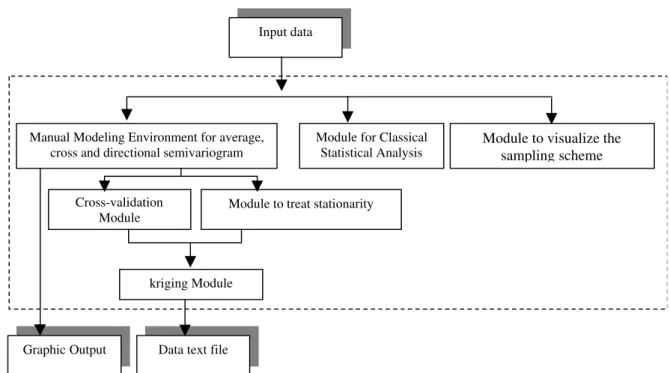
Figure 1 illustrates the modules developed in the current version of the system.
The system first verifies the possible lack of in-put parameters (name of the data file, maximum distance, LAG, etc.) and, if necessary, generates error messages or warnings. These data are then recorded in a text file, called parameter file (Figure 2c), which informs the ac-tions to be performed by the Fortran Program. Internally, the Delphi system evokes the Fortran Program. Next, the command line shows this call to the Fortran Program, which calculates the values of an experimental semivariogram (avar.exe):
WinExec(‘ avar.exe’, SW_HIDE );
Figure 1 - Diagram of the geostatistical system developed. Input data
Manual Modeling Environment for average, cross and directional semivariogram
Module for Classical Statistical Analysis
Module to treat stationarity Cross-validation
Module
Module to visualize the sampling scheme
kriging Module
The avar.exe program is executed within the DOS environment, producing a result text file. The Delphi sys-tem then reads the resulting file and presents it in a graphic and/or tabular form. Figure 2 depicts an example of the interaction between the Delphi system modules and the text files generated executing the FORTRAN routines. The kriging step used the Surfer software 7.0 to produce the soil maps.
Notions of continuity and of spatial dependence are associated to the semivariogram (Clark, 1979). Two
regional variables, X and Y, where X = Z(xi) and Y = Z(xi
+ h), are then considered and associated as coordinate pairs, (x1,y1) and (x2,y2), respectively, and separated by the lag or distance vector h (module and direction). The semivariogram is defined as:
γ(h) = 1/2 E{ Z (xi) - Z(xi + h)}2
(1)
that is, half of the mathematical expectation (E) of the square of the difference between the values of the points in a field, separated by a distance vector h. The equation
for the estimation γ* is given by:
(2)
where N(h) is the number of pairs of measured values
Z(xi) and Z(xi+h), separated by the vector h and Z(xi);
Z(xi+h) are values of observations of the regionalized
variable sampled at the points xi and xi+h.
A semivariogram that is practically uniform for all directions of the vector h denotes the presence of
isotropy within the spatial variability. Conversely, if the semivariogram is not the same for all directions, this characterizes an anisotropic distribution. Figure 3 exem-plifies a geometrical anisotropy where, for the same sill, directions 45º and 135º present ranges with different values.
Figure 3 presents the essential parameters of the semivariogram, which are:
• Nugget Effect (Co): when a semivariogram tends to zero
(γ (h) = 0) a value Co is observed, which reveals the
dis-continuity of the phenomenon for values smaller than the least distance between samples.
• Range (a): distance within samples are spatially corre-lated.
• Sill (C): value of γ which corresponds to the range (a)
on the graph of the semivariogram. It is considered that, from this point on, there is no more spatial dependence between the samples.
The next step is to adjust a mathematical model that best represents the configuration of the curve of the experimental semivariogram. The spherical (Sph), exponential (Exp) and Gaussian (Gau) models are rep-resented in Figure 4. These are basic models, which Isaaks & Srivastava (1989) called isotropic models with sill. Models with sill are known as transitive, that is, after a certain distance, the model reaches a maxi-mum and constant value. Other models reach the sill (C) asymptotically. There are also models with no sill, which correspond to the possibility of infinite dispersion of
Figure 2 - Generic scheme of interaction between the system modules and text files generated by the FORTRAN routines. (b) Parameter files
(c) Result file (d) Interface with output graphic
Execution of the Fortran Routine
Delphi system processing the Numerical Results (a) Interface for parameters input
a phenomenon. These phenomena do not have finite variance and their covariance may not be defined (Vieira, 2000).
Since the whole geostatistical analysis process involves uncertainty and subjectivity, one must assess the performance of the estimation in points where the val-ues are known. This estimation error assessment may be
performed using the procedure known as Jackknifing or
cross-validation. Vieira (2000) discusses the concepts in-volved in this technique in details.
Matheron (1963) pays a tribute to the South-Af-rican mining engineer Daniel G. Krige and his tion method, called kriging, which allows the interpola-tion of values in any posiinterpola-tion of the field studied, with-out bias and with minimum variance. Because of its weighed moving average, the kriging method resembles the interpolation method, but, since it determines the weights according to the spatial analysis provided by the experimental semivariogram, it diverges from the simple linear interpolation and Inverse Square of Distance meth-ods. The kriging estimator supplies unbiased estimations, that is, on the average, there is no distortion between the
estimated and actual values of a same point. Another im-portant characteristic is the minimum variance, which means that, although there may be differences between the estimated and measured values from point to point, these differences are very low.
As a linear estimator, a kriging procedure may be represented by the weighed linear combinations of mea-sured data, or a moving average that considers a variabil-ity structure of the measured variable, expressed by the semivariogram and by the localization of known values. In this concept, the points closest to the position that will be interpolated have a major weight in relation to the most distant ones.
The kriging estimator is formulated as follows:
( )
( )
i Ni
iZ x
x
Z
∑
=
=
1 0
* λ
(3)
where N is the number of measured values Z(xi) used in
the prediction, and λi is the weight associated to each
measured value Z(xi). The simple and ordinary krigings
are the most used techniques. For further details, see Journel (1989).
Data used in this study came from Waynick & Sharp (1919), which were later also used by Vieira (2000). The observations concern two fields in Califor-nia, USA, with almost invariant slope, one in the so-called University Farm, in Davis (clay loamy soil) and the other in the city of Oakley (sandy soil). One hundred soil samples were collected in each field.
The case study presented in this work is an analy-sis of Carbon (C), Nitrogen (N) and of the Carbon/Ni-trogen relationship in a rectangular grid (63.99 m x 81.89 m) with different densities in its edges and central parts. According to the authors, sampling sought to assess the variability of C and N in two apparently homogenous, al-luvial soils.
The spatial distribution of the sampled points is illustrated in Figure 5.
RESULTS AND DISCUSSION
The highest means and the maximum and mini-mum values of Carbon and Nitrogen correspond to the field in Davis (Table 1). Except for the variable C/N -Oakley, all other present low variance values, which means that most of the values are close to the mean.
The high values of the kurtosis coefficient rep-resent a more peaked frequency curve than the normal curve, which confirms the concentration of values close to the mean value. The 0.7637 index, between the mea-sures of Carbon and Nitrogen in the Oakley field, and the 0.6268 index between Carbon and Nitrogen in Davis, de-note mean positive correlations between these two vari-ables (Table 2).
Figure 4 - Theoretical models of semivariogram (Source: Camargo, 1997).
Figure 3 - Graphic representation of a geometrical anisotropy for two directions (a), according to the directional conventions (b) used in geostatistics.
(b) East 45 º
135 º
Range 1 Range 2
Theoretical models
Sill (C)
(
C0
)
North
South West
45 º
135 º
h γ(h)
Mean Variance C.V. Minimum Maximum Symmetry Coefficient Kurtosis C-Davis (g kg-1) 11.110 1.0900 9.394 8.960 13.83 0.464 -0.154
N-Davis (g kg-1) 0.998 0.008403 9.183 0.770 1.18 -0.254 -0.0183
C-Oakley (g kg-1) 4.330 1.3290 26.620 1.820 9.50 1.468 3.881
N-Oakley (g kg-1) 0.3208 0.0048 21.800 0.210 0.60 1.582 4.233
C/N-Davis (%) 11.170 0.9630 8.784 9.415 17.26 2.731 14.320
C/N- Oakley (%) 13.570 6.1060 18.210 7.857 23.23 0.926 3.055
C-Davis N-Davis C-Oakley N-Oakley C/N-Davis C/N-Oakley
C-Davis 1.0000 0.6268 0.0406 0.1362 0.4322 -0.1130
N-Davis 0.6268 1.0000 -0.0425 -0.0511 -0.4243 -0.0101
C-Oakley 0.0406 -0.0425 1.0000 0.7637 0.0925 0.5205
N-Oakley 0.1362 -0.0511 0.7637 1.0000 0.2224 -0.1337
C/N-Davis 0.4322 -0.4243 0.0925 0.2224 1.0000 -0.1333
C/N-Oakley -0.1130 -0.0101 0.5205 -0.1337 -0.1333 1.0000
Table 1 - Statistics for the dataset Waynick & Sharp (1919).
Table 2 - Correlation matrix.
Figure 5 - Spatial distribution of the points sampled in the two fields.
Modeling average semivariogram
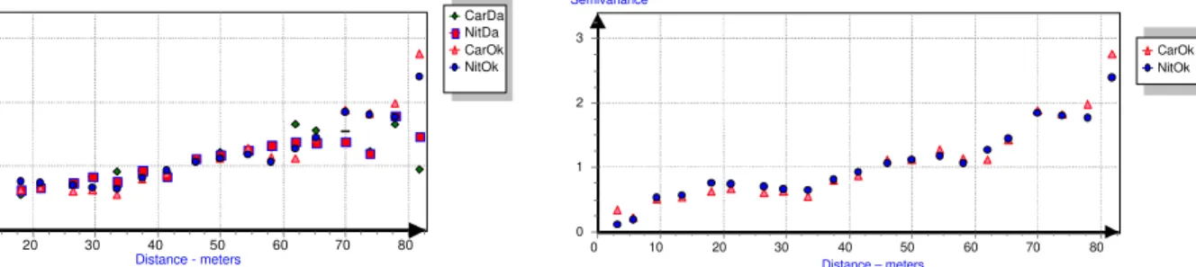
Figure 6 presents the scaled semivariograms of the Carbon and Nitrogen variables for the fields in Davis and Oakley. Scaling is obtained dividing each semivariogram point of the variables by its respective variance. This procedure allows to compare the spatial structure of the variables on a same scale, as used in Vieira et al. (1991). A preliminary visual analysis of Fig-ure 6 shows that the semivariance values between both variables (carbon and nitrogen) in the two sites, through-out the distance axis, are very close.
In the present study, the Carbon and Nitrogen variables in Oakley were chosen to perform a geostatistical analysis, since they presented the highest
Treatment of data stationarity
In this step, the parabolic trend surface was ap-plied to the unscaled semivariogram of the Carbon and Nitrogen variables in Oakley, as to subtract the effect of the infinite dispersion of the data. This operation resulted in a residue curve (Figure 8), which consists of the dif-ference between the values of the experimental semivariogram and the values of the trend surface. As it presents a graphic behavior similar to that of an ideal semivariogram, this curve is used, from now on, to ad-just the theoretical models, and in the cross-validation and kriging processes. Once interpolated, the values of the trend surface are summed up to the residues to reconsti-tute the data set that will yield the maps.
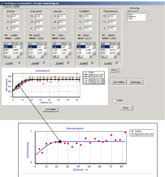
Adjusting the mathematical models
The system implements five kinds of mathemati-cal models to adjust the experimental semivariogram: spherical, exponential, Gaussian, Hole Effect and pentaspherical. Through the input of the theoretical model parameters (nugget effect – Co, structural variance – C1, and range – a), the respective curve is superimposed to the points of the experimental semivariogram.
The spherical model provided the best Multiple
correlation coefficient (R2) – close to one – and Weighed
Regression Sum of Square (WRSS) – least value (Figure 9). For Carbon, the values following parameters were ob-tained: nugget (Co) = 0.25; structural variance (C1) = 0.43; sill = 19.5 meters. The model best fitted to the semivariogram of Nitrogen residues was the spherical,
with the following parameters: C0 = 0.0; C1= 0.003, and
sill = 19 meters. In this step, the system reproduced a non-scaled experimental semivariogram. This approach allows the adjusted parameters to be in the natural scale of each variable semivariance.
Application of the of Cross-validation – JackKnifing
module
Using C0, C1 and range values of the section:
“Adjusting the mathematical models”, one obtains the es-timates of the cross-validation parameters presented in Tables 3 and 4. The neighborhoods that best estimated the parameters, according to the ideal parameters of each variable, were the 16 and 8 neighborhoods for Carbon and
Figure 7 - Scaled average semivariograms for Carbon and Nitrogen in the Oakley field.
CarOk NitOk
Distance – meters
80 70 60 50 40 30 20 10 0 3 2 1 0 Semivariance
Figure 6 - Scaled average semivariograms of Carbon and Nitrogen in the Davis and Oakley fields.
CarDa NitDa CarOk NitOk
Distance - meters
80 70 60 50 40 30 20 10 0 3 2 1 0 Semivariance
Figure 8 - Graph generated by the function Detrending (experimental semivariogram - , residue curve - ), for carbon (a) and nitrogen (b).
C-Oakley Residue Distance- meters 80 70 60 50 40 30 20 10 Semivariiance 2 1 0
Distance - meters
80 70 60 50 40 30 20 10 Semivariance 2 1 0 N-Oakley Residue A B
Nitrogen, for Oakley, respectively. These neighborhoods are considered as ideal for the kriging process.
Kriging
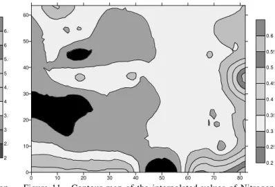
The system generated a text file with the esti-mated values in a one-meter square grid, to which the re-spective values of the estimate variance were added. The interpolated map for Carbon for Oakley (Figure 10) shows its major continuity or variability of value classes for the
direction – 45ºQ, a direction that presents the least
con-tinuity for the Nitrogen variable (Figure 8). The 0.3 to 0.35 values represent the class of major occurrence in the studied area (Figure 11).
CONCLUSIONS
Neighborhoods Reduced error variance (1) *
Reduced error
mean (0) Intersection (0)
Angular coefficient (1)
Correlation coefficient (1)
8 1.387 -0.02372 0.001070 0.7395 0.4215
12 1.413 -0.02815 0.0009622 0.6405 0.3798
16 1.535 -0.03278 0.001053 0.5906 0.3597
20 1.598 -0.01622 0.0006361 0.5778 0.3514
24 1.642 -0.01281 0.0005356 0.5730 0.3504
Table 4 - Estimate of the parameters of the cross-validation for data of Nitrogen residues - Oakley
* Ideal values of each parameter are in brackets. Neighborhoods Reduced error
variance (1) *
Reduced error
mean (0) Intersection (0)
Angular coefficient (1)
Correlation coefficient (1)
8 1.339 -0.03860 0.002929 0.08225 0.03243
12 1.329 -0.02142 0.002401 0.1086 0.04108
16 1.336 -0.01567 0.001671 0.09424 0.3551
20 1.342 -0.01391 0.001723 0.1077 0.04078
24 1.356 -0.02904 0.005836 0.07839 0.02974
Table 3 - Estimates of the cross-validation parameters for the Carbon residues data - Oakley
* Ideal values of each parameter are in brackets.
Figure 9 - Adjusting the mathematical models to the curve of Carbon residues for the Oakley soil, with details of the curve of the spherical model.
CaRes Sph(0,25-0,43-19,5) Semivariogram
Distance - m
80 70 60 50 40 30 20 10 0
Semivariance
1
model is also thought off as a future activity, in this sys-tem, to provide a comparison basis for the manual adjust-ment. Given its characteristic of quick prototypation and simplicity when incorporating correlated routines, the Delphi environment presents the main advantage of per-mitting the evolution of this system. The analysis of the dataset of Waynick & Sharp (1919) constituted an initial study and did not intend to deepen the results as for the agronomic issue. Still, the results obtained, mainly as re-gards to the interpolated maps, resemble those found by Vieira (2000). Further information on the use of this sys-tem may be found at: http://www.cnptia.embrapa.br.
REFERENCES
CAMARGO, E.C.G. Desenvolvimento, implementação e teste de procedimentos geoestatísticos (krigeagem) no sistema de processamento de informações georreferenciadas (SPRING). São José dos Campos: INPE, 1997. 146p. (Dissertação - Mestrado).
CLARK, I. Practical geostatistics. London: Applied Science Publishers, 1979. 130p.
DEUTSCH, C.V.; JOURNEL A.G. GSLIB: geostatistical software library and user’s guide. New York: Oxford University Press, 1998. 369p.
GEOSTATICAL SOFTWARE LIBRARY. http://www.gslib.com. (13 nov. 2001).
INPRISE CORPORATION. Borland Delphi 5 for Windows 98, Windows
95, & Windows NT: developer’s guide. Scotts Valley, 1999.
Figure 10 - Contour map of the interpolated values of Carbon (Oakley).
Received April 08, 2002 Accepted October 23, 2003
Figure 11 - Contour map of the interpolated values of Nitrogen (Oakley).
ISAAKS, E.H.; SRIVASTAVA, R.M. An introduction to applied
geostatistics. New York: Oxford University Press, 1989. 561p.
JOURNEL, A.G. Fundamentals of geostatistics in five lessons. Short Course in Geology. Washington: American Geophysical Union, 1989. 40 p.
MATHERON, G. Principles of geostatistics. Economic Geology, v.58, p.1246-1266, 1963.
OLIVER, M.A Geostatistics and its application to soil science. Soil Use
and Management, v.3, p.8-20, 1987.
PRESSMAN, R.S. Software engineering: a practitioner’s approach. New York: McGraw-Hill, 1982. 352p.
SPRING. http://www.dpi.inpe/spring. (4 fev. 2002).
VIEIRA, S.R. Geoestatística em estudos de variabilidade espacial do solo. In: NOVAIS, R.F. de; ALVAREZ V., V.H.; SCHAEFER, C.E.G.R. (Ed.)
Tópicos em ciência do solo. Campinas: Sociedade Brasileira de Ciência
do Solo, v.1, p.1-54, 2000.
VIEIRA, S.R.; LOMBARDI NETO, F.; BURROWS, I.T. Mapeamento da chuva máxima provável para o Estado de São Paulo. Revista Brasileira
de Ciência do Solo, v.15, p.93-98, 1991.
VIEIRA, S.R.; HATFIELD, T.L.; NIELSEN, D.R.; BIGGAR, J.W. Geostatistical theory and application to variability of some agronomical properties. Hilgardia, v.51, p.1-75, 1983.
WAYNICK, D.D.; SHARP, L.T Variability in soils and its significance to past and future soil investigations. II. Variation in nitrogen and carbon in field soils and their relation to the accuracy of field trials. Agricultural
Science, v.4, p.121-139, 1919.
0 10 20 30 40 50 60 70 80
0 10 20 30 40 50 60
2 2.5 3 3.5 4 4.5 5 5.5 6 6.5
0 10 20 30 40 50 60 70 80
0 10 20 30 40 50 60