Abstract—A strategy for dealing with turbulent flows over a two dimensional surface mounted obstacle using the wall y+ as guidance in selecting the appropriate grid configuration and corresponding turbulence models are investigated using Fluent. The CFD results were compared with experimental data from Zeidan’s Turbulent Shear Recovery behind Obstacles on Smooth and Rough Surfaces. Both undisturbed and disturbed (over ridge) flows are studied.
For both cases, a wall y+ in the range of 30 to 60 is determined to be sufficiently accurate, where the log-law region is resolved. It is also advisable to avoid having the wall-adjacent mesh in the buffer region since neither wall functions nor near-wall modeling approach accounts for it accurately. RSM predicts the flow properties more consistently because it accounts for all the Reynolds Stress components.
Keywords— Computation Fluid Dynamics, Fluent, turbulence, wall bounded flow, wall y+.
I. INTRODUCTION
HE majority of time spent on a Computation Fluid Dynamics (CFD) project in the industry is usually devoted to successfully generating a mesh for the domain geometry [1], that allows for a compromise between desired accuracy and solution cost. This time consuming process is considered a bottleneck in the analysis process.
The preferred procedure for determining the most accurate mesh is to carry out test runs on different mesh sizes and configurations until the numerical solution converges, in what is termed the grid independence test. Evidently, this requires a lot of time and computational effort.
Turbulent flows are significantly affected by the presence of walls, where the viscosity-affected regions have large gradients in the solution variables and accurate presentation of the near-wall region determines successful prediction of near-wall bounded turbulent flows. A strategy using the computed wall y+ is recommended when dealing with such flows as proposed by Gerasimov in his seminar titled Modeling Turbulent Flows using Fluent from ANSYS [2]. This assists in selecting the most suitable near-wall treatment (wall functions or near-wall modeling) and the corresponding turbulence model based on the wall y+.
Manuscript received December 3, 2008.
Salim .M. Salim (phone: 603-89248350; fax: 603-89248017; e-mail: [email protected]).
Cheah Siew Cheong (e-mail: [email protected]). All authors are with the School of Mechanical Manufacturing and Materials Engineering, Faculty of Engineering, University of Nottingham (Malaysia Campus), Jalan Broga, Semenyih, 43500 Selangor, Malaysia.
Undisturbed and disturbed turbulent flows over a flat plate, with and without a 2-D solid ridge, respectively, are simulated using Fluent 6.2 and the wall skin friction coefficient, Cf ,and mean velocity profiles are validated against reliable experimental data obtained by Zeidan [3].
The present study aims at drawing up recommendations for cases where experimental data might not be available for validation, including the behavior and suggested usage of the available models and near wall functions using Fluent. This serves to increase confidence of using commercial CFD package for industrial simulation instead of solely relying on experimentation, when dealing with wall-bounded complex turbulent flows.
II. NEAR WALL TREATMENT
Near-wall regions have larger gradients in the solution variables, and momentum and other scalar transports occur most vigorously [4]; and from Fig. 1 it can be observed that the viscosity-affected region (the inner layer in this case) is made up of three zones (with their corresponding wall y+), namely the:
Viscous sublayer (y+ 5)
Buffer layer or blending region (5 y+ ) Fully turbulent or log-law region (y+ 30 to 60) The wall y+ is a non-dimensional distance similar to local Reynolds number, often used in CFD to describe how coarse or fine a mesh is for a particular flow. It is the ratio between the turbulent and laminar influences in a cell.
Very close to the wall, viscous damping reduces the tangential velocity fluctuations, while kinematic blocking reduces the normal fluctuations. Towards the outer part of the near-wall region, however, the turbulence is rapidly augmented by the production of turbulent kinetic energy due to the large gradients in mean velocity.
Accurate presentation of the flow in the near-wall region determines successful prediction of wall-bounded turbulent flows. Values of y+close to the lower bound (y+≈30) are most desirable for wall functions whereas y+≈1 are most desirable for near-wall modeling [2].
Wall y
+
Strategy for Dealing with Wall-bounded
Turbulent Flows
Salim .M. Salim, and S.C. Cheah
Fig. 1 Subdivisions of near-wall region
The k- , RSε and δES turbulence models are primary valid for turbulent core flows (somewhat far from walls); and hence are coupled with wall functions to bridge them with the solution variables in the viscosity-affected region.
Spalart-Allmaras and k-ω are by design applicable throughout the boundary layer, provided near-wall mesh resolution is sufficient. Hence, need for near-wall modeling.
III. UNDISTURBED FLOW
The computation domain, as illustrated by Fig. 2, was chosen to mimic the experimental work carried out by Zeidan for an undisturbed flow with zero-pressure gradient over a smooth surface. Air enters the flow domain perpendicular to the wall with uniform velocity. Symmetry, which is essentially a wall with slip condition, is chosen for the above boundary to reduce computational time, as the height of the domain is sufficiently far to influence the flow over the surface of interest, i.e. the bottom wall.
Fig. 2 Computation flow domain and boundary conditions
RSM was used in the grid test. Three different mesh sizes are applied in the grid test, as illustrated in Fig. 3, to introduce the idea of wall y+ as a means of identifying the appropriate near-wall treatment (wall functions or near-wall modeling). This is achieved by refining the mesh, with particular attention
to the near-wall region so as to achieve the above wall y+, i.e. the distance from the wall to the centroid of the wall-adjacent cells.
As seen in Fig. 4, the corresponding wall y+ values are: y+≈32.5 (log-law region)
y+≈17.5 (buffer region) y+≈2.5 (viscous sub layer)
Fig. 3 Mesh configuration for undisturbed flow
Fig. 4 Corresponding wall y+
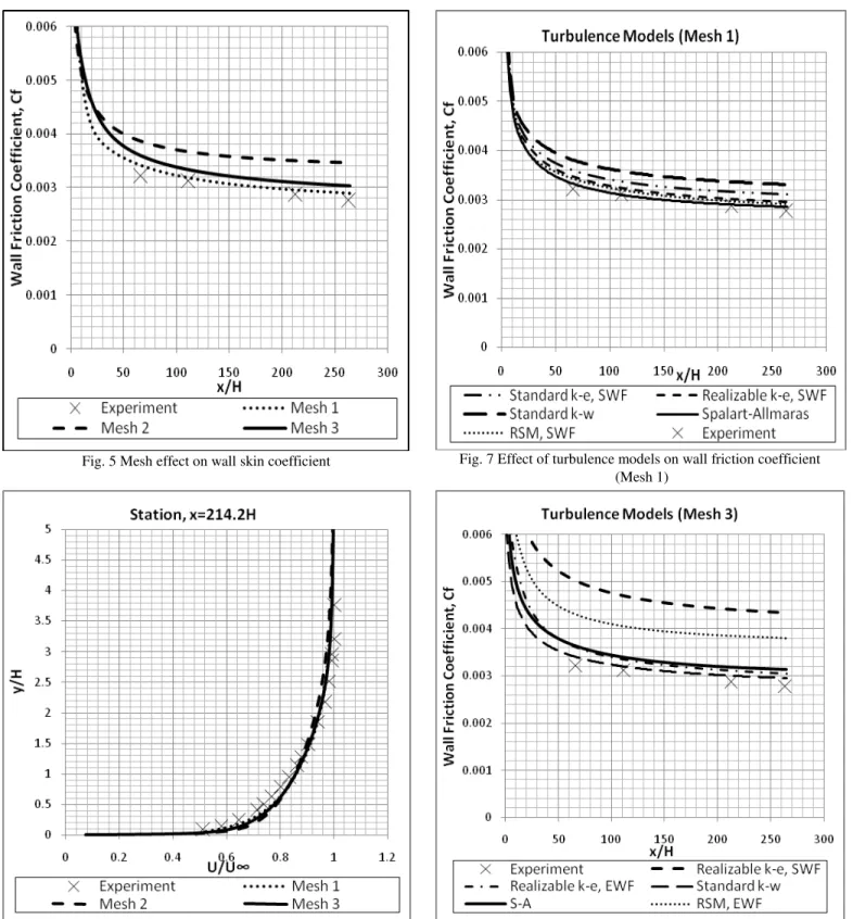
The different mesh configurations and corresponding wall y+ have a significant influence on the computed wall friction coefficient results as shown in Fig. 5, but minimal effect on the mean velocity profile as can be seen in Fig. 6.
Mesh 1 (3000 cells)
Mesh 2 (4000 cells)
Mesh 3 (10600 cells) Proceedings of the International MultiConference of Engineers and Computer Scientists 2009 Vol II
Fig. 5 Mesh effect on wall skin coefficient
Fig. 6 Mesh effect on velocity profile
Referring to Fig. 5, mesh configurations that have wall y+ values resolved in the buffer region, i.e. 5<y+<30 (Mesh 2 [max error 20.22%]) tend to exhibit less accuracy in Cf -predictions as compared to those resolving the viscous sublayer or log-law region (Mesh 1 [max error 6.27%] and Mesh 3 [max error 11.86%], respectively).
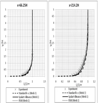
Fig. 7 Effect of turbulence models on wall friction coefficient (Mesh 1)
Fig. 8 Effect of turbulence models on wall friction coefficient (Mesh 3)
From the grid test, it was determined that Mesh 1 [max error 6.27%] gave the best accuracy followed by Mesh 3. Mesh 2 is discarded due to its large deviation. Turbulence models are tested using Mesh 1 and Mesh 3 as shown in Fig. 7 and Fig. 8, respectively, to highlight the different approaches required for the near-wall treatment.
[max error 6.27%] and Spalart-Allmaras [max error 5%], whereas for Mesh 3 (Fig. 8), it is Standard k-ω [5.87%]. Some interesting trends in the turbulence model behavior are also observed in Fig. 7 and Fig. 8. For example, RSM works well in Mesh 1 but deviated significantly in Mesh 3, whereas the Standard k-ω model improves in Mesh 3 in comparison to Mesh 1.
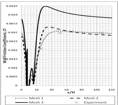
Again, the effect of turbulence models on the mean velocity profiles at two downstream locations is minimal as shown in Fig. 9.
The above comparison of results can be explained in terms of the turbulence model itself and the near-wall treatment approach it is coupled with. RSM is primary valid for turbulent core flows as it is coupled with wall functions (semi-empirical formulas usually approximating the log-law region). Hence, it works well when the wall-adjacent cells are in the log-law region (as in Mesh 1) but the accuracy is severely affected when the cells are resolved in the viscous sublayer since the log-law formulae ceases to be valid [4]. This is equally true for k- .
Unlike RSM, the k-ω and Spalart-Allmaras models are designed to be applied throughout the boundary layer provided that the near-wall mesh resolutions are sufficient (with no added wall-functions necessary to bridge them to the wall). That is why their accuracy increased as the cell sizes (and correspondingly the wall y+) reduced, because more details (i.e. the viscous sublayer) is captured during computation.
Fig. 9 Effect of turbulence models on velocity profile (Mesh 1)
IV. DISTURBED FLOW-FLOW OVER RIDGE
Similar to the undisturbed flow, the computational flow domain illustrated by Fig. 10 was chosen to mimic the experiment done by Zeidan for a flow over a ridge bounded by a smooth surface. The obstacle (ridge) is placed at a distance x=112.5 H from the inlet, where the boundary layer thickness
has grown to ≈2H, with H being the height of the obstacle.
Fig. 10 Computational flow domain and boundary conditions
Parallel to the undisturbed flow study, three different mesh sizes are applied to investigate the concept of wall y+ as a means of identifying the suitable near-wall treatment (wall functions or near-wall modeling). The mesh configurations and corresponding wall y+ chosen for the flow domain are illustrated in Fig. 11 and Fig. 12, respectively, and are as follows:
y+≈50 (log-law region) y+≈12.5 (buffer region) y+≈2.5 (viscous sub layer)
The drop and spikes in wall y+ are expected due to the presence of an obstruction (ridge) in the flow path [5].
Fig. 11 Mesh configuration for disturbed (over ridge) flow Mesh 1 (5822 cells)
Mesh 2 (9138 cells)
Mesh 3 (19393 cells) Proceedings of the International MultiConference of Engineers and Computer Scientists 2009 Vol II
Fig. 12 Corresponding wall y+
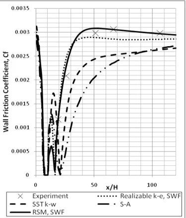
The grid test is done using the RSM turbulence model coupled with Standard Wall Function (SWF). The noticeable thing in Fig. 13 is that the model chosen failed to predict the wall friction coefficient appropriately for Mesh 3. This could be explained in terms of the y+, which is laminar ( i.e. resolving the viscous sublayer) and as previously determined, the wall functions cease to be valid in that region.
Mesh 1, gave the best approximation [max error 4.03%] and the recommendation to avoid refining the mesh into the buffer region is confirmed as seen by the result of Mesh 2 (y+ ≈12, buffer region).
Interestingly, as concluded in the undisturbed flow study, the mesh choices does not matter much when predicting the velocity profiles as observed in Fig. 14.
Fig. 13 Mesh effect on wall friction coefficient
Fig. 14 Mesh effect on velocity profile
Comparison of the computational results with experimental data for Mesh 1(shown in Fig. 15) further emphasizes the relationship between the mesh size (using the y+ parameter) and near wall treatment for each turbulence model. Starting off with the general trends, it is observed that RSM and Realizable k- (both using SWF) give better Cf-predictions than the S-A (Spalart-Allmaras) and SST (Shear Stress Transport) k-ω models. As discussed earlier, RSM and k- are core-turbulent models and need to be bridged to the near-wall region using wall functions which work best in the log-law region. Contrary to that, S-A and k-ω are designed to be valid throughout the boundary layer, hence the need for fine mesh resolution (i.e. near-wall modeling).
As for the two core-turbulent models (i.e. between RSM and k- ), RSε performs better because it accounts for each Reynolds Stress component unlike k- , which assumes them to be isotropic. But if computation time and effort are limited, then k- is an acceptable choice, since RSε takes roughly twice the number of iterations to reach convergence.
Fig. 15 Effect of turbulence model on wall friction coefficient (Mesh 1)
Fig. 16 Effect of turbulence model on wall friction coefficient (Mesh 3)
V. CONCLUSION
The present study shows that the non-dimensional wall y+ is a suitable selection criterion for determining the appropriate mesh configuration and turbulence model, coupled with near-wall treatment, that lead to accurate computational predictions in Fluent.
A mesh size that resolves the log-law (fully turbulent) region is sufficient for computation, without incurring added time or effort by refining into the viscous sublayer. It is also advisable to avoid resolving the buffer (mixing) region as neither wall functions nor near-wall modeling accounts for it accurately.
REFERENCES
[1] T. Jinyuan, H.Y. Guan, and L. Chaoqun, Computation Fluid Dynamics:
A Practical Approach . USA: Butterworth-Heinemann, 2006, pp. 35–
37.
[2] A. Gerasimov, “εodeling Turbulent Flows with FδUENT,” Europe,
ANSYS,lnc. 2006.
[3] A. Zeidan, “Turbulent Shear Flow Recovery Behind Obstacles on
Smooth and Rough Surfaces,” PhD Thesis. Dept. Mech. Eng.,
University of Liverpool, UK, 1980.
[4] Fluent 6.2 Documentation File, ANSYS Manual, 2006.
[5] R. Bashakaran, and C. Lance, “Introduction to CFD,” New York, Cornell University.