Rafael Gabler Gontijo
[email protected] Universidade de Brasília - Departamento de Engenharia Mecânica Vortex - Mecânica dos Fluidos de Escoamentos Complexos Brasília 70910-900 DF, Brazil
José Luiz Alves da Fontoura
Rodrigues
[email protected] Universidade de Brasília - Departamento de Engenharia Mecânica Vortex - Mecânica dos Fluidos de Escoamentos Complexos Brasília 70910-900 DF, Brazil
The Numerical Modeling of Thermal
Turbulent Wall Flows with the Classical
κ
−
ε
Model
The goal of this work is to propose a new methodology to simulate turbulent thermal wall flows using the classicalκ−εmodel. The focus of this approach is based on the manner used to implement heat flux boundary conditions on the solid walls. In order to explain and to validate this new algorithm, several test cases are presented, testing a great range of flows in order to analyze the numerical response on different physical aspects of the fluid flow. The proposed approach uses simultaneously a thermal wall law, an analogy be-tween fluid friction and heat transfer and an interpolating polynomial relation that is con-structed with a data base generated on experimental research and numerical simulation. The algorithm used to execute the numerical simulations applies the classicalκ−εmodel with a consolidate Reynolds and Favre averaging process for the turbulent variables. The turbulent inner layer can be modeled by four distinct velocity wall laws and by one tem-perature wall law. Spacial discretization is done by P1 and P1/isoP2 finite elements and the temporal discretization is implemented using a semi-implicit sequential scheme of fi-nite differences. The pressure-velocity coupling is numerically solved by a variation of Uzawa’s algorithm. To filter the numerical noises, originated by the symmetric treatment of the convective fluxes, it is adopted a balance dissipation method. The remaining non-linearities, due to explicit calculations of boundary conditions by wall laws, are treated by a minimal residual method.
Keywords:turbulence, finite element method, wall laws, analogies, turbulent heat flux
Introduction
Thermal turbulent flows over solid surfaces occur in many sit-uations of industrial interest and the thermal boundary conditions imposed on the boundaries of the computational grid may be of two types: temperature and/or heat flux. The second condition is more usual in real problems and it brings some additional difficulties to its numerical treatment.
According to Chen and Jaw (1998), the high Reynolds κ−ε
model is the most used turbulence model in the treatment of indus-trial flows. To model the behavior of the flow in the internal region of the turbulent boundary layer, theκ−εmodel uses analytical ex-pressions known as wall laws. The main difficulty in simulating a thermal turbulent flow with a heat flux boundary condition on the wall using the high Reynoldsκ−εmodel is the absence of a heat flux wall law.
The method that we propose to solve this inconvenience is to calculate the convective heat transfer coefficienth, along the solid boundary, and use its value to convert an imposed heat flux on an equivalent wall temperature. This information is then sent to a tem-perature wall law that calculates the temtem-perature boundary condition in the nodes placed on the border of the computational grid.
The main difficulty is to estimate, with a good accuracy, the nu-merical values of the convective heat transfer coefficient, since it strongly depends on the flow and on features like the thermodynam-ical properties of the fluid, the solid geometry in which the flow occurs and the Reynolds number of the flow. In this work, for
non-Paper accepted August, 2010. Technical Editor: Eduardo Morgado Belo
detached boundary layers, the values of hare calculated with the use of analogies between fluid friction and heat diffusion. For de-tached boundary layers the calculation is done using an interpolating polynomial relation.
The good performance of classical analogies used to calculate heat transfer rates on flat plates was shown by Gontijo and Fon-toura Rodrigues (2006). The problem of using analogies between fluid friction and heat diffusion in detached boundary layers was dis-cussed in the work of Gontijo and Fontoura Rodrigues (2007). An original approach based on the use of analogies for solving the prob-lem of imposing heat flux boundary conditions on the high Reynolds
κ−εmodel was first presented by Gontijo and Fontoura Rodrigues (2008) and an evolution of this method was shown by Gontijo and Fontoura Rodrigues (2009). The present work shows how this new and original method can be used to simulate thermal turbulent flows with heat flux boundary conditions over different geometries.
The solver used to execute the simulations, named Turbo 2D, is a research Fortran numerical code that has been continuously developed by members of the Group of Complex Fluid Dynamics -Vortex, of the Mechanical Engineering Department of the Univer-sity of Brasilia, in the last twenty years. This solver is based on the adoption of the finite elements technique, under the formulation of weighted residuals proposed by Galerkin, adopting in the spatial dis-cretization of the calculation domain triangular elements of the type P1 and P1-isoP2, as proposed by Brison, Buffat, Jeandel and Serres (1985). The P1-isoP2 mesh is obtained dividing each element of the P1 mesh into four new elements. In the P1 mesh only the pressure field is calculated, while all the other turbulent variables are calcu-lated with the P1-isoP2 mesh.
Considering the uncertainties normally existing about the ini-tial condition of the flow field, it is adopted a temporal integration scheme of the governing equations system. In the temporal inte-gration process, the initial state corresponds to the beginning of the flow and the final state occurs when temporal variations of veloc-ity, pressure, temperature and other turbulent variables stop. In or-der to reach the final state a pseudo transient occurs. The temporal discretization of the governing equations is implemented by the al-gorithm of Brun (1988), wich uses a sequential semi-implicit finite differences method with truncation error of order0(∆t)and allows a linear handling of the equation system, at each time step.
The resolution of the coupled equations of continuity and mo-mentum is done by a variant of Uzawa’s algorithm, proposed by Buffat (1981). The statistical formulation, used for obtaining the system of average equations, is done with the simultaneous employ-ment of the Reynolds (1895) and Favre (1965) decomposition. The Reynolds stress tensor is calculated by the hypothesis of the turbu-lent viscosity of Boussinesq (1877), wich is modeled by theκ−ε
model, proposed by Jones and Launder (1972) with the modifica-tions introduced by Launder and Spalding (1974). The turbulent heat flux is modeled algebraically using a turbulent Prandl number with a constant value of 0.9.
In the program Turbo 2D, the boundary conditions of velocity and temperature can be calculated by four velocity and two tem-perature wall laws. The velocity wall functions used in this work are: the classical logarithm law, and the laws of Mellor (1966), Nakayama and Koyama (1984), and Cruz and Silva Freire (1998). The temperature wall law used is the Cheng and Ng (1982) law. The numerical instability resultant of the explicit calculation of veloc-ity boundary conditions is controlled by the algorithm proposed by Fontoura Rodrigues (1990). The numerical oscillations induced by the Galerkin formulation, resultant of the centered discretization ap-plied to a parabolic phenomenon, are cushioned by the technique of balanced dissipation, proposed by Huges and Brooks (1979) and Kelly, Nakazawa and Zienkiewicz (1976) with the numerical algo-rithm proposed by Brun (1988).
In order to validate and quantify the consistence of the present research code, the numerical results are compared with an extensive experimental database, including several flows over distinct geome-tries, based on the works of Ng (1981), Vogel and Eaton (1985), Taylor et al. (1990), Liou et al. (1992), Buice and Eaton (1995) and Loureiro et al.(2007).
Nomenclature
t time variable
xi spacial variable - component in theidirection ui fluid velocity
e
ui velocity’s mean value by Favre’s decomposition u′′i velocity fluctuation by Favre’s decomposition u∞ velocity of the free stream flow
uf friction velocity T fluid temperature
e
T temperature’s mean value by Favre’s decomposition
T∞ temperature of the free stream flow
Tf friction temperature Tw wall temperature p pressure
¯
p mean pressure by Fravre’s decomposition
qi′′ heat flux vector qw′′ heat flux on the wall k fluid’s thermal conductivity
Cp specific heat at constant pressure gi gravitational acceleration vector
D
Dt Material’s derivative operator R ideal gas constant
K Von Karman’s constant
α fluid’s thermal conductivity
αt turbulent thermal conductivity ρ fluid’s density
¯
ρ density mean value by Reynolds decomposition
ρ′′ density’s fluctuations
τij shear stress tensor in indicial notation τw shear stresses on the wall
κ turbulent kinetic energy
ε dissipation of turbulent kinetic energy
ν kinematic viscosity
νt dynamic turbulent viscosity µ dynamic viscosity
µt turbulent dynamic viscosity β volumetric expansion coefficient
δij Kronecker’s delta operator F r Froude number
M a Mach number
N u Nusselt number
P r Prandtl number
P rt turbulent Prandtl number Re Reynolds number
Ret turbulent Reynolds number St Stanton number
y+ Reynolds number of the turbulent boundary layer
Theoretical Formulation
Governing Equations
In this work all the dependent variables of the fluid are treated as a time average value plus a fluctuation in a determinate point of space and time. In order to account variations of density, the model applies the well known Reynolds (1985) decomposition to pressure and fluid density and the Favre (1965) decomposition to velocity and temperature. In the Favre (1965) decomposition a generic variable
ϕis defined as:
ϕ(~x, t) =ϕe(~x) +ϕ′′(~x, t)
with
e
ϕ= ρϕ
¯
ρ and ϕ
′′
Applying the Reynolds (1895) and Favre (1965) decompositions to the governing equations and taking the time average value of those equations, we obtain the mean Reynolds equations:
∂ρ
∂t +
∂ ∂xi
(ρeui) = 0, (2)
∂
∂t(ρuei) + ∂ ∂xj
(ρuejeui) =−∂p ∂xi
+ ∂
∂xj
h
τij−ρu′′ju′′i
i
+ρgi, (3)
where
τij =µ
∂ e
ui ∂xj
+∂euj
∂xi
−2
3
∂uel ∂xl
δij
, (4)
∂(ρTe)
∂t +
∂(ueiTe) ∂xi
= ∂
∂xi α∂Te
∂xi
−ρu′′ iT′′
!
(5)
p=ρRTe (6)
In this system of equations,ρis the fluid density,tis time,xiare
the space cartesian coordinates in index notation,µis the dynamic viscosity coefficient, αis the molecular thermal diffusivity, δij is
the Kronecker’s delta operator,giis the acceleration due to gravity, T is the fluid temperature,ui is the flow velocity,kis the thermal
conductivity,pis the fluid pressure andτ is the fluid stress tensor. In these equations the tilde denotes the time-average of a quantity whereas quotation marks denote the fluctuation of a quantity in the sense of Favre (1965) decomposition. Similarly, overbar denotes the time-average of a quantity in the sense of Reynolds (1985) de-composition. Two new unknown quantities appear, respectively, in the momentum (3) and in the energy equations (5), defined by the correlations between velocity fluctuations, the so-called Reynolds Stress, given by the tensor−ρu′′
iu′′j, and by fluctuations of
temper-ature and velocity, the so-called turbulent heat flux, defined by the vector−ρu′′
iT′′.
The Reynolds stress of turbulent tensions is calculated by the
κ−εmodel, proposed by Jones and Launder (1972) with the modi-fications introduced by Launder and Spalding (1974), given by
−ρu′′
iu′′j =µt
∂uei
∂xj +
∂euj ∂xi
−2
3
ρκ+µt∂uel ∂xl
δij, (7)
with
κ= 1
2u′′iu′′i. (8)
and
µt=Cµρ¯κ
2
ε =
1
Ret
. (9)
The turbulent heat flux is modeled using the Fourrier law and a turbulent Prandl numberP rtequal to a constant value of 0.9 by the
relation:
−ρu′′ iT′′=
µt P rt
∂Te ∂xi
. (10)
In Eq. (9)Cµis a constant of calibration of the model, equal to
0.09,κrepresents the turbulent kinetic energy andεis the rate of dis-sipation of the turbulent kinetic energy. Onceκandεare additional variables, we need to know the transport equations. The transport equations ofκandεwere deduced by Jones and Launder (1972), and the closed system of equations of theκ−εmodel is given by:
∂ρ¯
∂t +
∂(¯ρeui)
∂xi = 0
, (11)
∂(¯ρuei)
∂t +uej
∂(¯ρeui) ∂xj
=−∂p¯∗
∂xi
+∂x∂
j h 1 Re+ 1 Ret ∂eui ∂xj +
∂euj ∂xi
i
+F r1 ρg¯ i , (12)
∂ρ¯Te
∂t +euj
∂ρ¯Te
∂xj = ∂ ∂xj h 1
Re P r +
1
RetP rt
∂Te ∂xj
i
, (13)
∂(¯ρκ)
∂t +uei ∂(¯ρκ)
∂xj = ∂ ∂xi 1 Re ∂κ ∂xi + ∂ ∂xi 1
Retσκ ∂κ ∂xi
+ Π−ρε¯ + ρβg¯ i RetP rt
∂Te ∂xi , (14)
∂(¯ρε)
∂t +eui ∂(¯ρε)
∂xj = ∂ ∂xi 1 Re ∂ε ∂xi + ∂ ∂xi 1
Retσε ∂ε ∂xi
+ ε
κ(Cε1Π−Cε2ρε¯ )
+κεCε3Reρβg¯tP ri t∂x∂Tei
, (15)
¯
ρ1 +Te= 1 , (16)
where:
1
Ret
= Cµρ¯κ
2
ε , (17)
Π = 1
Ret
∂uei ∂xj
+∂uej
∂xi
∂eui ∂xj
−23ρκ¯ +Re1t∂eul ∂xl
p∗ = p¯+2
3 1
Re +
1
Ret
∂ e
ul ∂xl
+ ¯ρκ
(19)
with the model constants given by:
Cµ= 0,09, Cε1= 1,44, Cε2= 1,92,
Cε3= 0,288, σκ= 1, σε= 1,3, P rt= 0,9.
Wall Functions
Theκ−εturbulence model is uncapable of properly represent-ing the laminar sub-layer and the transition regions of the turbulent boundary layer. To solve this inconvenience, the solution adopted in this work is the use of wall laws, capable of properly representing the flow in the inner region of the turbulent boundary layer.
There are four velocity and two temperature wall laws imple-mented on the code Turbo 2D. The laws used in this simulation are explained bellow, except for the classical log law whose further ex-planations are unnecessary.
Velocity wall law of Mellor (1966)
Deduced from the mean equation of Prandtl for the turbulent boundary layer and considering the pressure gradient term for inte-gration, this wall function is a primary approach to flows that suffer influence of adverse pressure gradients. Its equations are, respec-tively, for the laminar and turbulent regions
u∗=y∗+1
2p
∗y∗2 , (20)
u∗= 2
K
p
1 +p∗y∗−1
+K1 4y
∗
2+p∗
y∗
+2√1+p∗
y∗
+ξp∗ , (21)
where the asterisk upper-index indicates dimensionless quantities of velocityu∗, pressure gradientp∗and distance to the wally∗as
func-tions of scaling parameters at the near wall region, K is the Von Karman constant andξp∗ is Mellor’s integration constant which is a
function of the near-wall dimensionless pressure gradient.
For calculation purposes the intersection of both regions is con-sidered to be the same as the log law expressions, where y∗ =
11,64. The relations between the dimensionless near wall proper-ties and the friction velocityuf are:
y∗= y uf
ν ,u
∗= eux uf
and p∗=1
¯
ρ ∂p¯
∂x ν uf3
. (22)
The friction velocity is calculated by the relation:
uf =
1
Re +
1
ReT
∂ui ∂xj
−1
ρ ∂P ∂xi
δij (23)
In Eq. (21) the termξp∗ is a value obtained from the integration
process proposed by Mellor (1966) and is a function of the dimen-sionless pressure gradient. Its values are obtained through interpo-lation of those obtained experimentally by Mellor, shown in Table 1.
Table 1. Mellor’s integration constant (1966).
p∗ −0.01 0.00 0.02 0.05 0.10 0.20
ξp∗ 4.92 4.90 4.94 5.06 5.26 5.63
p∗ 0.25 0.33 0.50 1.00 2.00 10.00
ξp∗ 5.78 6.03 6.44 7.34 8.49 12.13
Velocity wall law of Nakayama and Koyama (1984)
In their work Nakayama and Koyama (1984) proposed a deriva-tion of the mean turbulent kinetic energy equaderiva-tion, that resulted in an expression to evaluate the velocity near solid boundaries. Us-ing experimental results and those obtained by Strattford (1959), the derived equation is
u∗= 1
K∗
3(t−ts) +ln
ts+ 1 ts−1
t−1
t+ 1
, (24)
with
t=
r 1 + 2τ∗
3 , τ
∗= 1 +p∗y∗,
K∗= 0,419+0,539p∗
1+p∗ and y∗s=
eK C
1+p∗0,34, (25)
whereK∗ is the expression for the Von Karman constant modified
by the presence of adverse pressure gradients,τ∗is a dimensionless
shear stress,C= 5.445is the log-law constant and the parameterts
is a value of t at a positiony∗ s.
Velocity wall law of Cruz and Silva Freire (1998)
Analyzing the asymptotic behavior of the boundary layer flow under adverse pressure gradients, Cruz and Silva Freire (1998) derived an expression for the velocity in the inner region of turbulent boundary layer. The solution of the asymptotic approach is
u= τw
|τw|
2
K
s
τw
ρ +
1
ρ dpw
dx y+
τw
|τw| uf
Kln
y
Lc
with Lc =
q
(τw ρ )
2
+2ν ρ
dpw dx uf−τwρ 1
ρdpwdx
(26)
where the sub-indexwindicates the properties at the wall, K is the
Von Karman constant,Lcis a length scale parameter anduf is the
The proposed equation for the velocity, equation (26), has a be-havior similar to the log law far from the separation and reattach-ment points, but, close to the separation point, it gradually tends to Stratford’s equation (1959).
Temperature wall law of Cheng and Ng (1982)
In this work it is used the temperature wall law of Cheng and Ng (1982). For the calculation of the temperature profile in the near wall region, Cheng and Ng (1982) derived an expression similar to the logarithmic law for velocity. For the laminar and turbulent regions, the equations are respectively
(T0−T)y Tf
=y∗P r and
(T0−T)y
Tf =
1
KN gln(y
∗) +CN g
with y∗=ufy
ν (27)
whereT0is the environmental temperature,yis the normal distance
up to the wall,ν is the cinematic viscosity and Tf is the friction
temperature, as defined by Brun (1988)
Tf = 1
uf
" 1
ReP r+
1
ReTP rT
∂Te ∂xj
#
δ
, (28)
and the friction velocityufis calculated by Eq. (23).
The intersection of these regions are aty∗= 15,96and the
con-stantsKN gandCN g are, respectively,0,8and12,5.
The Heat Flux Boundary Condition And The
κ
−
ε
Model
As discussed before, imposing a heat flux boundary condition on the wall in a high Reynolds turbulence model, such as the classical
κ−ε, requires a special treatment since there are no heat flux wall functions available. This work proposes a new method to solve this inconvenience without the need of creating a heat flux wall law. The main idea is to use the Colburn (1933) analogy, Eq. (29), to estimate the Stanton number for non-detached boundary layers.
Stx=
Cf x
2P r23
, (29)
whereCfxis the local friction coefficient and the local Stanton
num-ber can be evaluated by
Stx=
qx ρcpu∞(Tw−T∞)
, (30)
where, for a flat plate
qx=−k
∂T
∂y
y=0
. (31)
By Eq. (30) it is possible to convert an imposed heat flux on the wall into an equivalent wall temperature by knowing the behavior of the local Stanton number, since
Tw=T∞+
qx ρCpu∞Stx
. (32)
If there is an unheated starting length, so the thermal boundary layer begins its development under a pre-existing velocity boundary layer an adjustment is necessary to take into account this peculiarity of the flow. The adjust proposed by Kays and Crowford (1993) can be done on Eq. (29) resulting in the Eq. (36),
Stx=
Cf x
2P r23
δ
u δT
1 7
, (33)
where δu and δT denotes, respectively, the velocity and thermal
boundary layer thickness.
In equation (30) an accurate calculation of the temperature gra-dient is a difficult task since the use of wall laws produces the loss of some information in the wall region. On the other hand, this dif-ficulty can be avoided by employing equations (29) or (36), where the local friction coefficient Cfx is calculated with the use of the
friction velocityuf, wich is calculated by equation (23), so:
Cf x
2 =
τw ρu2
∞
with τw=ρu2f
and Cf x= 2 u2
f u2
∞. (34)
By these calculations it is possible to estimate, with a good ac-curacy, the heat transfer rates in turbulent flows where the boundary layer is well structured, for example, in flows over flat plates and other geometries that don’t generate boundary layer detachment.
The problem in using this formulation happens when we analyze the flow inside or at downstream of a recirculation region, where the boundary layer is not well structured and the use of analogies is not a viable alternative. In these cases, Gontijo and Fontoura Ro-drigues (2009) developed an expression using a previously experi-mental work of Vogel and Eaton (1985), where the authors studied a turbulent flow over a heated backward facing step that had a condi-tion of a constant heat flux imposed on its lower wall. The relacondi-tion obtained is expressed by Eq. (35).
St(x∗) = 0,00106 + 0,00912x∗−0,00895x∗2+ 0,00233x∗3,
with
x∗= x−xd
xr−xd,
(35)
wherexdefines the local coordinate in the flow direction,xdis the
detachment point andxris the reattachment point.
Results
Several test cases were used to validate this methodology in or-der to show its generality. First it is shown the good performance of analogies in cases where there is no boundary layer detachment. Following are addressed problems of using classical analogies when the boundary layer is not well structured. Thereafter, it is shown the arguments taken into account to develop a new approach to cal-culate the Stanton number inside a recirculation region and, finally, this approach is tested for different geometries that induce boundary layer detachment. A mesh study was done for each test case and more details on the numerical process can be found in the Master’s Dissertation of Gontijo (2009).
Use of analogies on flat plates with unheated starting lengths and low temperature gradients
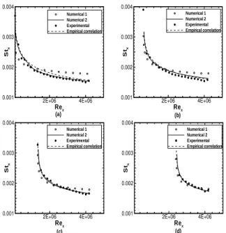
First it is shown the performance of the Colburn analogy in the estimation of the local Stanton number for four different test cases, based on the experimental works of Taylor et al. (1990). In this work the authors made several measurements of the local Stanton number over a heated flat plate. The plate had2.4mlong. The flow is considered two-dimensional in the midle section and the velocity of the free stream flow isU∞ = 28m/s. The results presented in Fig. (1) show the behavior of four different test cases, varying the initial unheated starting length.
Rex
S
tx
2E+06 4E+06 0.001
0.002 0.003 0.004
Numerical 1 Numerical 2 Experimental Empirical correlation
(a)
Rex
S
tx
2E+06 4E+06 0.001
0.002 0.003 0.004
Numerical 1 Numerical 2 Experimental Empirical correlation
(b)
Rex
S
tx
2E+06 4E+06 0.001
0.002 0.003 0.004
Numerical 1 Numerical 2 Experimental Empirical correlation
(c)
Rex
S
tx
2E+06 4E+06 0.001
0.002 0.003 0.004
Numerical 1 Numerical 2 Experimental Empirical correlation
(d)
Figure 1. Local Stanton number for Taylor et al. (1990) test case.
U∞ = 28 - Isothermal plate (a), ξ=0,36 m (b), ξ=0,76 m (c) and ξ=1,36 m (d).
In the legend the experimental result is obtained from the work of Taylor et al. (1990), empirical correlation denotes the Kays and
Crowford (1993) correlation, given by
Stx=
Cfx
2P r2/3 "
1−
ξ
x
9/10#−1/9
, (36)
wherexis the distance from the beginning of the plate andξis the unheated starting length. The numerical value of the local Stanton number was calculated by two different ways, using Eqs. (30) and (36) called in Fig. (1), respectively, numerical 1 and numerical 2. The main idea of the works of Taylor et al. (1990) is to evaluate the influence of a thermal boundary layer starting over a developed velocity boundary layer in the behavior of the heat transfer rates over a plate with low temperature gradients. In these cases, there is a difference of18Kbetween the temperature of the plate and of the free stream flow. The numerical P1-isoP2 mesh used to execute the simulations had 18447 nodes and 35872 elements. In this case the wall law used for velocity was the classic logarithm law and for temperature the wall law of Cheng and Ng (1982), since there are no significative pressure gradients imposed by this geometry. It is possible to notice that the use of the Colburn (1933) analogy calcu-lated by Eq. (36) produces better results. The explanation for this behavior consists on the fact that the derivatives of temperature in the normal direction of the plate are not taken on the wall, since the use of a high Reynolds model restrict the numerical simulation to a certain distance above it.
Analogies in an isothermal flat plate with high temperature gradients
In order to validate the use of the Colburn (1933) analogy in problems where the temperature and velocity fields are coupled due to a high temperature gradient, a simulation of a problem first stud-ied by Ng (1981) is presented. In this test case a flat plate of0.25m
long, heated in a constant temperature of 1250K, receives a flow of air with a free stream velocity of10,7m/sand with an uniform temperature of293K. In this work the range of the local Reynolds number is placed between5.0 105 < Re
x < 7.8 105. There is a
difference of957Kbetween the temperature of the plate and of the free stream flow. It was used a P1-isoP2 mesh with 6499 nodes and 12672 elements. The simulation was done with the classic wall law for velocity and the wall law of Cheng and Ng (1982) for temper-ature. Figure (2) shows the variation of the local Stanton number through the plate calculated by the same way as those from the Tay-lor et. al (1990) test case.
In the legend of Fig. (2) the experimental values are taken from the work of Ng (1981) and the numerical values are obtained by the same way that in the Taylor et al. (1990) test case. The behavior ob-served is the same, the use of the Colburn (1933) analogy calculated by Eq. (36) is the best option to estimate the heat transfer rates. It is important to notice that the Colburn analogy works well even when the temperature gradients involved are very strong.
The use of analogies in a recirculation region
X (m)
S
tx
0 0.05 0.1 0.15
0.002 0.003 0.004 0.005
Numerical 1 Numerical 2 Experimental
Figure 2. Local Stanton number for Ng (1981) test case.
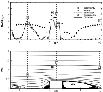
was selected a test case based on the works of Liou et al. (1992). In this test case, artificial roughness elements calledribsare used to induce the flow separation, increasing the turbulence levels and, by consequence, the heat transfer rates. The ribbed channel studied in this work presents a Reynolds number of 12600. The velocity on witch the Reynolds number was calculated is7.4m/sand the height of the rib is0.008m. The P1-isoP2 mesh used on the simulations had 3739 nodes and 7200 elements. In the experimental work of Liou et al. (1992), the rib was made of aluminum and it was heated by a thermal film in its underside, providing a condition of constant heat flux. The top part of the channel was insulated, so an adiabatic wall was created. The height of the rib represents twenty percent of the height of the channel. Figure (3) shows the behavior of the heat transfer rates along the channel. In the legend of Fig. (3) the experimental values are taken from the work of Liout et al. (1992).
X/h
Y
/h
-1 0 1
0 0.5 1 1.5 2
(b) A
B C
D
x/h
N
u
/N
u
_
s
0 1 2 3 4 5 6
experimental log law Mellor’s law Koyama’s law CSF’s law
-1 0 1 (a)
A
B C
D
Figure 3. Nusselt number along the bottom wall (a), structure of the recirculation regions (b).
In this work, the wall heat flux is calculated in the non
dimen-sional form of the Nusselt number that for a channel can be calcu-lated by the following relation:
N ux= 2qxP rH
µCp(Tw−Tbulk)
(37)
In the equation above,N uxrepresents the local Nusselt number, qx is the local heat flux,P r is the Prandtl number of the fluid, H
is the height of the channel, andTwis the temperature of the wall.
Combining Eq. (37) with the Colburn (1933) analogy, Eq. (30), and with the definition of the local Stanton number, where the bulk temperature may be taken as
Tbulk =
Tw+T∞
2 , (38)
it is possible to establish a relation between the local Nusselt number and the friction velocity as
N ux=
4P r13u2
f xH
νu∞
. (39)
The values ofN us, shown in Fig. (3), are the local Nusselt
num-bers for a channel without the presence of the Ribs, calculated by the Dittus-Boeltter equation. It is possible to observe a good agreement between numerical and experimental data in non detached regions (places A, B and C). Inside the recirculation zones, the use of the Colburn analogy does not present good results. This was already ex-pected, since analogies between fluid friction and heat transfer can only be done in a well structured boundary layer. The results of Fig. (3) show the necessity of an alternative treatment to estimate, with a good accuracy, the behavior of the local Stanton number in regions of the flow where the boundary layer is not well structured, like in-side recirculation zones and after the reattachment of the boundary layer, as the following test case will illustrate.
An approach to estimate the Stanton number in detached flows
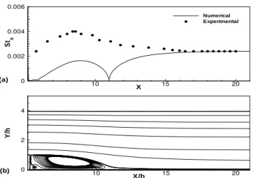
In order to propose a new methodology to estimate the local Stanton number inside a recirculation region, the experimental work of Vogel and Eaton (1985) was set as the benchmark to develop this approach. In this test case a backward facing step, with a height of
0.038m is heated in the bottom plate with a constant heat flux of
270W/m2. The Reynolds number based on the height of the step
is 27023. The free stream velocity of the flow is 11.3m/s. The P1-isoP2 mesh used to execute the simulation has 4191 nodes and 8016 elements. Figure (4) shows the behavior of the local Stanton number when calculated by the use of the Colburn analogy. This be-havior suggests that after the reattachment point the boundary layer is being restructured. This restructure occurs in a region that has approximately the same length of the recirculation region.
X/h
Y
/h
10 15 20
0 2 4
(b)
X
S
t
10 15 20
0 0.002 0.004 0.006
Numerical Experimental
(a)
x
Figure 4. Numerical and experimental behavior of the Stanton num-ber (a), streamlines of the flow (b).
X/h
S
t
5 10 15 20
0 0.002 0.004
0.006 This approach
Experimental
x
Figure 5. Adjusts obtained by the proposed relation.
the detachment point to a distance of twice the recirculation zone length, based on the physical reality of the backward facing step of Vogel and Eaton. This relation is given by Eq. (35). By using this equation the behavior of the local Stanton number, in a simulation done with the Cruz and Silva Freire wall law, is shown in Fig. (5). The adjust obtained with Eq. (35) shows a good accuracy between numerical and experimental values and the transition from the use of this equation to the calculation with the Colburn analogy is smooth, after the restructuring region of the boundary layer. It is important to say that the necessary length for the boundary layer restructuring is still an open problem and needs further studies. However, this methodology turns viable the simulation of turbulent thermal flows with the high Reynoldsκ−εmodel with wall laws and heat flux boundary conditions. In order to validate this methodology to other geometries with boundary layer detachment, the next section shows its performance in an asymmetric plane diffuser and on a smooth hill.
Extension of this new approach to other detached flows in-duced by different geometries
In order to extend this methodology to other geometries, two new test cases were proposed, based on studies of the asymmetric plane
diffuser of Buice and Eaton (1995) and the turbulent flow over a 2D hill, studied by Loureiro et al. (2007). The boundary conditions used to execute these simulations are illustrated in Figs. (6) and (7).
Figure 6. Geometry and boundary conditions of the Buice and Eaton (1995) diffuser.
Figure 7. Geometry and boundary conditions of the Loureiro et al. (2007) 2D hill.
T
Y
/h
0 0.01 0.02 0.03 0
0.2 0.4 0.6 0.8 1
Expected profile This approach
(b) T
Y
/h
0 0.1 0.2 0
1 2 3
4 Expected profileThis approach
(a)
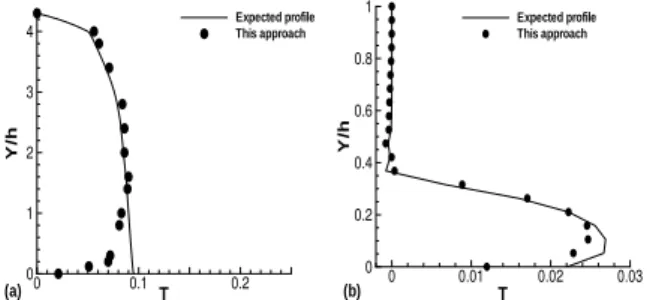
Figure 8. Temperature profiles in the asymmetric diffuser of Buice and Eaton (1995) - X/h=26 (a) and in the 2D hill of Loureiro et al.
(2007) in X/h=6.5 (b).
Figure (8) illustrates, respectively, the temperature profiles taken after the heated walls for the asymmetric plane diffuser of Buice and Eaton (1995) and the 2D hill of Loureiro et al. (2007) test cases. The expected profile line indicates a temperature profile taken when an equivalent constant temperature is imposed, more details are given in the master’s dissertation of Gontijo (2009). This approach is able to predict the equivalent wall temperature in-side the recirculation regions of flows over distinct boundary ge-ometries, even when the mechanism responsible by the bound-ary layer detachment is a very smooth adverse pressure gradi-ent. More details over the proccess of development of this new methodology are given by Gontijo and Fontoura Rodrigues (2009). It is important to notice that the temperature profiles should not be exactly the same when simulations are taken using a constant tem-perature and a constant heat flux boundary condition, even if the en-ergy injected by both boundary conditions is the same. The enen-ergy injected in the flow, associated with the integral of the temperature profile should be the same instead. The error on the energy injected by both boundary conditions, obtained with this methodology based on the physical reality of the backward facing step and extended to other geometries is0.21%for the diffuser and0.06%for the smooth hill.
Conclusions
This work proposed, implemented and validated, successfully, a original numerical methodology used to impose heat flux boundary conditions in the high Reynoldsκ−εmodel, without the need to create a heat flux law of the wall. Past works done by the authors were used to develop this methodology based on the employment of classical analogies between fluid friction and heat transfer on the wall. The test case used to develop this methodology and also to understand the main obstacles of this approach was the Vogel and Eaton (1985) backward facing step. The advances done based in this test case were then tested in two other geometries and showed that this methodology can be extended to distinct geometries, even when the detached is induced by smooth adverse pressure gradients. One of the aspects that can be better studied is the necessary length to the restructuring of the boundary layer after the detachment, even though in the studied test cases the adopted standard considered in
this work has provided good results.
Acknowledgements
The authors are grateful by the support given by the Conselho Nacional de Desenvolvimento Científico e Tecnológico, CNPq and by the professors, students and members of the research group Vor-tex - Group of Fluid Mechanics of Complex Flows of the University of Brasília.
References
Boussinesq, J., 1877, “Théorie de l’écoulement Tourbillant”, Mem. Présentés par Divers Savants Acad. Sci. Inst. Fr., Vol. 23, pp. 46-50.
Buffat, M., 1981, “Formulation moindre carrés adaptées autraite-ment des effets convectifs dans les équation de Navier-Stokes”, Doc-torat thesis, Université Claude Bernard, Lyon, France.
Buice, C. and Eaton, J., 1995, “Experimental investigation of flow through an asymmetric plane diffuser”, Annual Research Briefs - 1995, Center of Turbulence Research, Stanford University/ NASA Ames, pp. 117-120.
Brison ,J.F., Buffat, M., Jeandel, D., Serrer, E., 1985, “Finite el-ements simulation of turbulent flows, using a two equation model”, Numerical methods in laminar and turbulent flows, Swansea. Piner-idg Press.
Brun, G., 1988, “Developpement et application d’une methode d’elements finis pour le calcul des ecoulements turbulents fortement chauffes”, Doctorat thesis, Laboratoire de Mécanique des Fluides, Ecole Centrale de Lyon, France.
Chen, C.J. and Jaw, S.Y., 1998, “Fundamentals of Turbulence Modeling”, Taylor and Francis, New York.
Cheng, R.K. and Ng, T.T., 1982, “Some aspects of strongly heated turbulent boundary layer flow”,Physics of Fluids, Vol. 25(8). Colburn, A.P., 1933, “A method for correlating forced convec-tion heat transfer data and a comparison with fluid fricconvec-tion”, Trans-action of American Institute of Chemical Engineers, Vol. 29, pp. 174-210.
Cruz, D.O.A., Silva Freire, A.P., 1998, “On single limits and the asymptotic behavior of separating turbulent boundary layers”,
International Journal of Heat and Mass Transfer, Vol. 41,No 14,
pp. 2097-2111.
Favre, A., 1965, “Equations de gaz turbulents compressibles”,
Journal de mecanique, Vol. 3 and Vol. 4.
Fontoura Rodrigues, J.L.A., 1990, “Méthode de minimisation adaptée à la techinique des éléments finis pour la simulation des écoulements turbulents avec conditions aux limites non linéaires de proche paroi”, Doctorat thesis, Ecole Centrale de Lyon, France.
Gontijo, R.G. and Fontoura Rodrigues, J.L.A., 2006, “Numerical modeling of the heat transfer in the turbulent boundary layer”, Encit, 2006.
Gontijo, R.G. and Fontoura Rodrigues, J.L.A., 2007, “Numerical modeling of a turbulent flow over a 2D channel with a rib-roughened wall”, Cobem, 2007.
boundary conditions in a high Reynolds turbulence model”, Encit, 2008.
Gontijo, R.G. and Fontoura Rodrigues, J.L.A., 2009, “Thermal boundary conditions based on the use of analogies. A numerical study”, Cobem, 2009.
Huges, T.J.R. and Brooks, A., 1979, “A multi-dimensional up-wind scheme with no crossup-wind diffusion”, in “Finite Element Methods foConvection Dominated Flows”, ASME - AMD 34, New York.
Jones, W. and Launder, B.E., 1972, “The prediction of lami-narization with a two equations model of turbulence”,International Journal of Heat and Mass Transfer, Vol. 15, pp. 301-314.
Kays, W.M., Crawford, M.E., 1993, “Convective Heat and Mass Transfer”, McGraw Hill, INC., USA.
Kelly, D.W., Nakazawa, S., Zienkiewiczs, O.C., Heinrich, J., 1976, “A note on upwind and anisotropic balancing dissipation in finite element approximations to convective diffusion problems”, In-ternational Journal for Numerical Method in Engineering,15, Vol. 11, pp.1705-1711.
Launder, B.E. and Spalding, D.B., 1974, “The numerical compu-tation of turbulent flows”,Computational Methods in Applied Me-chanical Engineering, Vol. 3, pp. 269-289.
Loureiro, J.B.R, Soares, D.V, Fontoura Rodrigues, J.L.A, Silva Freire, A.P, Pinho, F.T, 2007, “Water tank and numerical model stud-ies of flow over 2-D hill”,Boundary Layer Meteorology, Vol. 122, Serie 2 , pp.343-365.
Mellor, G.L., 1966, “The effects of pressure gradients on turbu-lent flow near a smooth wall”,Journal of Fluid Mechanics, Vol. 24,
No2, pp. 255-274.
Nakayama, A., Koyama, H., 1984, “A wall law for turbulent boundary layers in adverse pressure gradients”,AIAA Journal, Vol. 22,No10, pp. 1386-1389.
Reynolds, O., 1895, “On The Dynamical Theory of Incompress-ible Viscous Fluids and the Determination of the Criterion”, Philo-sophical Transactions of the Royal Society of London, Series A, Vol. 186, p. 123.
Taylor, R.P. , Love, P.H. , Coleman, H.W. and Hosni, M.H., 1990, “Heat Transfer Measurements in Incompressible Turbulent Flat Plate Boundary Layers With Step Wall Temperature Boundary Conditions”,Journal of Heat Transfer, Vol. 112, pp 245-247.
Vogel, J.C., Eaton, J.K., 1985, “Combined heat transfer and fluid dynamic measurements downstream of a backward-facing step”,