Open Plot Project: an open-source toolkit for 3-D structural data analysis

(1)

SED

2, 375–385, 2010

Open Plot Project

S. Tavani et al.

Title Page

Abstract Introduction

Conclusions References

Tables Figures

◭ ◮

Back Close

Full Screen / Esc

Printer-friendly Version Interactive Discussion

Discussion

P

a

per

|

Dis

cussion

P

a

per

|

Discussion

P

a

per

|

Discussio

n

P

a

per

|

Solid Earth Discuss., 2, 375–385, 2010 www.solid-earth-discuss.net/2/375/2010/ doi:10.5194/sed-2-375-2010

Solid Earth Discussions

This discussion paper is/has been under review for the journal Solid Earth (SE). Please refer to the corresponding final paper in SE if available.

Open Plot Project: an open-source toolkit

for 3-D structural data analysis

S. Tavani, P. Arbues, M. Snidero, N. Carrera, and J. A. Mu ˜noz

Geomodels, Departament de Geodinamica i Geofisica, Facultat de Geologia, Universitat de Barcelona, Barcelona, Spain

Received: 12 November 2010 – Accepted: 1 December 2010 – Published: 6 December 2010 Correspondence to: S. Tavani (stefano.tavani@ub.edu)

(2)

SED

2, 375–385, 2010

S. Tavani et al.

Title Page

Tables Figures

◭ ◮

Back Close

Full Screen / Esc

Discussion

P

a

per

|

Dis

cussion

P

a

per

|

Discussion

P

a

per

|

Discussio

n

P

a

per

|

Abstract

In this work we present the Open Plot Project, a software for structural data analysis including a 3-D environment. This first alpha release represents a stand-alone toolkit for structural data analysis and, due to many import/export facilities and to the presence of a 3-D environment, also candidates as a tool to be incorporated in workflows for 3-D 5

geological modelling.

The software (for both Windows and Linux O.S.), the User Manual, a set of exam-ple movies, and the source code are provided as Supexam-plement. It is our purpose that the publication of the source code sets the base for the development of a public and free software that, hopefully, the structural geologists community will use, modify, and 10

implement. The creation of additional public controls/tools is strongly encouraged.

1 Introduction

In the last years the rising availability of new technologies and high-quality 3-D seismic data has implied the increasing use of truly 3-D geological models. Contextually, new methodologies have been developed to integrate surface and sub-surface geological 15

data to build geologically constrained 3-D models (e.g. Fern ´andez et al., 2004; Carrera et al., 2009; Jessel et al., 2010). However, information used for building 3-D mod-els commonly includes a limited suite of available data, particularly for data collected in the field. The geometries of geological surfaces, like faults and layers, are by far considered the most important data. Methodologies for the construction of geologi-20

cal models rarely incorporate other information, like the attributes of the deformation pattern, which can be crucial for extrapolating data into the undersampled portions of the aimed model (e.g. Thorbjornsen and Dunne, 1997; Tavani et al., 2006). More-over, the tools for structural data analysis implemented in commonly used 3-D CAD-like geological modelling software, have limitations in the interactive data selection, man-25

(3)

SED

2, 375–385, 2010

S. Tavani et al.

Title Page

Tables Figures

◭ ◮

Back Close

Full Screen / Esc

Discussion

P

a

per

|

Dis

cussion

P

a

per

|

Discussion

P

a

per

|

Discussio

n

P

a

per

|

data. Robust methodologies for 3-D reconstruction based on consistent bedding data interpolation and extrapolation require the use of in-house developed tools (e.g. Car-rera et al., 2009). In addition, widely used software for structural data analysis do not incorporate 3-D tools (or these are quite basic) and the “communication” between 3-D modelling software and structural data analysis tools is frequently neither simple 5

nor direct. Therefore, the whole process of 3-D reconstruction requires frequent and time-consuming passages between different CAD-like tools, software for structural data analysis, and in-house developed routines (e.g. Fern ´andez, 2004).

In this work we present the Open Plot Project software, a stand-alone structural data analysis software including a 3-D tool for data managing. The intents of Open 10

Plot Project are: (1) reducing the gap between CAD-like software for 3-D modelling and structural data analysis tools, and (2) providing an advanced toolkit for structural data analysis. The software is entirely written in RealBasic 2009r2 (RealSoftware Inc, 2009), a multi-platform basic language (running on Linux, Windows and Mac), which includes a 3-D control and represents an optimal compromise between speed, 3-D 15

graphic quality and programming easiness. The last point is particularly important to us, as the main intent of Open Plot Project is that of providing an open source code (the code is here provided as Supplement). A set of functionalities are provided in this first release being, however, the main purpose that of inviting the structural geology community to modify/implement the code, returning it to the community.

20

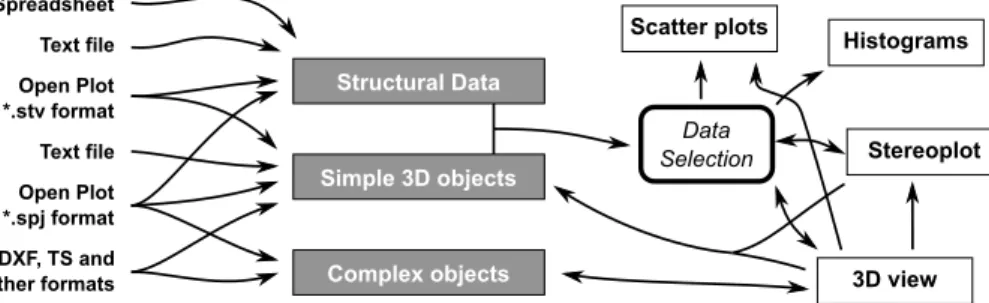
2 Summary of software architecture and functionalities

The complete description of functions and procedure for importing, saving, managing and exporting data is illustrated in the User Manual, which is attached to this work. In this section we summarise the internal workflow of the software.

The working philosophy of Open Plot Project is schematically illustrated in Fig. 1. 25

(4)

SED

2, 375–385, 2010

S. Tavani et al.

Title Page

Tables Figures

◭ ◮

Back Close

Full Screen / Esc

Discussion

P

a

per

|

Dis

cussion

P

a

per

|

Discussion

P

a

per

|

Discussio

n

P

a

per

|

– Structural data are punctual objects and include lineations, planes (eventually with slickenlines), and tensors. For these elements each record can include user-defined attributes. As an example, a joint with associated spacing, orientation, author, date, lithological information, etc., is a structural datum.

– Basic 3-D objects include “simple” 3-D surfaces (i.e. planar polygons and vertical 5

panels/multipanels), polylines, vectors and triangles. The record associated with vectors, triangles, polygons and polylines can include user-defined attributes and, in all the cases, orientation data are computed for them. On the contrary, vertical multipanels are purely geometrical objects with no attributes. These are used to create and save selections, drape images (like seismic sections or geological 10

cross sections), and to project structural data along the multipanel trace (i.e. to create structural transects, e.g. Wise and McCroy, 1982; Tavani et al., 2006).

– Complex objects include triangular meshes and images. In particular, three types of images can be loaded. (1) Textures: non-georeferenced images, which can be draped on vertical panels. (2) Map: georeferenced images, which can be draped 15

on meshes. (3) Image lists: arrays of images (typically photos of outcrops).

Structural data and basic 3-D objects can be saved in both *.stv and *.spj format. On the contrary, complex objects can be saved only in *.spj format. The first format is, in few words, a N×M matrix of strings, with an initial header where the number of columns and rows is specified. Such a format allows to easily import an *.stv file in 20

a spreadsheet, modify and re-import it in Open Plot Project (with a simple copy and paste procedure). Data editing and modification in external spreadsheets is thus rec-ommended, although a data editing tool is provided within the software. The structure of *.spj files is, in its first part (where structural data and basic 3-D objects are stored), identical to that of *.stv files. In the second part of the file points and triangles of 25

(5)

SED

2, 375–385, 2010

S. Tavani et al.

Title Page

Tables Figures

◭ ◮

Back Close

Full Screen / Esc

Discussion

P

a

per

|

Dis

cussion

P

a

per

|

Discussion

P

a

per

|

Discussio

n

P

a

per

|

Structural data and basic 3-D objects can be selected by filtering their attributes, and plotted in five windows: Frequency analysis, 2-D Scatterplot, 3-D Scatterplot, Stereoplot and 3-D View. In the first three cases a new matrix, including only the se-lected portion of the dataset, is generated. This new matrix is sent to the corresponding plotting window, just for data displaying and analysis, not for editing or modification. In 5

the case of stereoplot, the corresponding temporary matrix is linked to the main one and many operations can be performed on the selected portion of the dataset. These include the selection of a new sub-dataset, the assignation of new attributes, and the “storage” of directions that can be used in the 3-D View window to create new data. The functionalities of the 3-D View window are much more complex. Structural data, 10

basic 3-D objects, and complex objects can be displayed in this window. Similarly to the Stereoplot window, the displayed objects are linked to the main matrix. Basic 3-D objects can be created/erased here (also with the aid of tools present in the Stereoplot window) and many operations can be performed on the selected dataset. These op-erations include the projection of data along panels and the selection of sub-dataset, 15

which can be directly sent to the other plotting windows.

As previously described, structural data and basic 3-D objects can be directly im-ported in a spreadsheet by opening the corresponding *.stv file. Many 3-D objects, including polylines, meshes and planar polygons can be exported in *.DXF format.

Additional functionalities, which do not require the loading of data, are present in 20

Open Plot. Like, for example, the computation of fault slip direction from Riedel struc-tures (Riedel, 1929).

3 System requirements

Open Plot Project derives from a basic software developed to work in the field with the first low-cost netbooks. Open Plot Project preserves the capability of its ancestor of 25

(6)

SED

2, 375–385, 2010

S. Tavani et al.

Title Page

Tables Figures

◭ ◮

Back Close

Full Screen / Esc

Discussion

P

a

per

|

Dis

cussion

P

a

per

|

Discussion

P

a

per

|

Discussio

n

P

a

per

|

and Ubuntu8.04 or higher OS (it “should” also run in other Linux distribution, provided

that GTK +2.8 is installed and the window version run on Linux under Wine). The

version for Mac OS is not provided. However, Mac users can easily compile the code. Although most of the windows are correctly displayed on 800×480 screens, a minimum screen resolution of 1024×600 is recommended.

5

4 Case studies

In this section is briefly illustrated the application of Open Plot Project in two case studies. The procedures described in these examples can be followed in the relatives movies, provided in the Supplement, named Sibillini.mp4 and Pobla.mp4, respectively. The first example is from the Sibillini anticline, Northern Apennines (Italy). The 10

“structural” problem is that of evaluating the variability of pressure solution cleavage frequency in different structural positions of an anticline characterised by a variable axis orientation. The input dataset is from a spreadsheet including measurements col-lected in the field, like cleavage strike, dip, spacing and, as in this anticline the cleavage is stratabound, the thickness of the hosting layer. Scatterplot of cleavage spacing (S₎

15

vs. host-layer thickness (H_{) shows that these parameters are related and, accordingly,} H_/S _{should be used to quantify the cleavage frequency (e.g. Tavani et al., 2006). The}

*.stv file is thus imported in a spreadsheet, a new column is added, named “./HvsS” (the “./” characters will indicate the software that this is a numeric field), and the num-ber of columns is updated in the header. Now the entire file, including reserved fields 20

(see user manual) and the header, is copied. Import from clipboard procedure will recognise the header, and will load data without passing through the “boring” import procedure. In the data selection window bedding surfaces and pressure solution cleav-ages are selected and then plotted in the 3-D window. To evaluate the variability of cleavage HvsS across the fold strike, data have to be projected onto an across-strike 25

(7)

SED

2, 375–385, 2010

S. Tavani et al.

Title Page

Tables Figures

◭ ◮

Back Close

Full Screen / Esc

Discussion

P

a

per

|

Dis

cussion

P

a

per

|

Discussion

P

a

per

|

Discussio

n

P

a

per

|

region and send the data included in this region (both bedding and cleavage data) to the stereoplot. Here a tensorial analysis is performed only on bedding data. In the tensorial analysis results, we click “apply K3”, this assigns to entire selected dataset (including cleavages) the orientation of the local best-fit cylindrical axis. The same op-erations are performed for another region. We end up with two regions with di_fferent 5

cylindrical axes. Data now are projected onto the across-strike panel using “eigen-vector” option, such that, data are projected using the local axis orientation. A new 2-D scatterplot window will open up, including data that have been previously selected (i.e. bedding surfaces and cleavages). Two new attributes are added to each datum, namely the X and Z coordinates along the panel. In this scatterplot window we plot the 10

“X-position along panel” versus “HvsS”, result shows that cleavage frequency varies along the panel (i.e. across the fold) and, in particular, it roughly decreases toward the central portion of the transect (i.e. in the crestal sector).

The second example is from La Pobla de Segur (Spanish Pyrenees). Here it is il-lustrated how Open Plot can be used to create dip-domains. Traces were previously 15

digitalised onto a georeferenced orthophoto draped on a DEM. In the planar regres-sion tab of the drawing options window we define the parameters for the trace analysis procedure. This is a recursive procedure that finds, for each selected polylines group, a set of best-fit dip-domains (see user manual). In this window we also activate the dip-domains evaluation option, which will allow us to evaluate the “quality” of the au-20

(8)

SED

2, 375–385, 2010

S. Tavani et al.

Title Page

Tables Figures

◭ ◮

Back Close

Full Screen / Esc

Discussion

P

a

per

|

Dis

cussion

P

a

per

|

Discussion

P

a

per

|

Discussio

n

P

a

per

|

5 Discussion and conclusions

The possibility of easily import different data types from spreadsheets, text files, and other file formats, including meshes and polylines from DXF files, coupled with the simple STV file structure and the presence of a DXF export facility, allow to: (1) easily use Open Plot Project as a sort of structural add-on of CAD software, (2) use Open 5

Plot together with other structural tools; (3) use it as a stand-alone toolkit.

In the first case, Open Plot Project represents an external add-on allowing to import from di_fferent sources and manage together both georeferenced structural data and 3-D objects (like meshes and polylines), thus allowing to bypass the limitations of many CAD-like software in the import and management of “structural” data. These limita-10

tions can include, for example, the di_fficulties in making spatial or attribute queries, the difficulties in importing user-defined data attributes, the possibility of customizing the extraction of dip-domains from polylines, the handling of axial surfaces, and the defini-tion of projecdefini-tion direcdefini-tions. These and others limitadefini-tions can be partially (even totally) bypassed by acquiring specifically-developed add-ons that, however, in the most part 15

of the cases are neither free nor open source. Consistent and structurally-validated dip-domains created within Open Plot Project can be exported as DXF meshes and then imported in CAD software, where tools not present in Open Plot Project can be used to create and manage consistent volumetric models from these and other information. The possibility of selecting data according to (1) user-defined numeric and alphanu-20

meric attributes, (2) spatial distribution, and (3) attitude, together with the possibility of digitalising vectors and polylines on DEM or georeferenced images (including ge-ological map), allows to “export” selected data also toward structural software includ-ing analysis tools not yet implemented in Open Plot Project (like fault data inversion). Once a sub-dataset is selected, if data are saved as *.stv, the state (i.e. selected or 25

(9)

SED

2, 375–385, 2010

S. Tavani et al.

Title Page

Tables Figures

◭ ◮

Back Close

Full Screen / Esc

Discussion

P

a

per

|

Dis

cussion

P

a

per

|

Discussion

P

a

per

|

Discussio

n

P

a

per

|

On the other hand, the presence of widely-used data analysis tools (stereonets, ten-sorial regression, histograms with frequency analysis tools, 2-D and 3-D scatter-plots with data density contouring, transect analysis), efficient and different filtering options, 3-D environment, rather fast import/export procedures, coupled with the intrinsic ad-vantages of an open source software, support the use of Open Plot Project as the 5

main platform for data management.

Supplementary material related to this article is available online at:

http://www.solid-earth-discuss.net/2/375/2010/sed-2-375-2010-supplement.zip.

Acknowledgements. This work was carried out with the financial support of the Repsol-YPF, the MODES-4D (CGL2007-66431-C02-125 02/BTE) project and the “Grup de Recerca de

10

Geodin `amica i An `alisi de Conques” (2001SRG-126 000074). Susanne Buiter is thanked for editorial handling.

References

Carrera, N., Mu ˜noz, J. A., and Roca, E.: 3-D reconstruction of geological surfaces by the equiv-alent dip-domain method: an example from field data of the Cerro Bayo Anticline (Cordillera

15

Oriental, NW Argentine Andes), J. Struct. Geol., 31, 1573–1585, 2009.

Fern ´andez, O.: Reconstruction of geological structures in 3-D, An example from the southern Pyrenees, Ph.D. thesis, University of Barcelona, 2004.

Fern ández, O., Mu ñoz, J. A., Arbu és, P., Falivene, O., and Marzo, M.: Three-dimensional reconstruction of geological surfaces: An example of growth strata and turbidite systems

20

from the Ainsa basin (Pyrenees, Spain), AAPG Bull., 88, 1049–1068, 2004.

Jessell, M. W., Ailleres, L., and De Kemp, E. A.: Towards an integrated inversion of geoscientific data: What price of geology?, Tectonophysics, 490, 294–306, 2010.

RealSoftware Inc.: Realbasic 2009r2. Austin, Texas, USA, 2009.

Riedel, W.: Zur mechanik geologischer brucherscheinungen, Zentralblatt f ¨ur Mineralogie,

Ge-25

(10)

SED

2, 375–385, 2010

S. Tavani et al.

Title Page

Tables Figures

◭ ◮

Back Close

Full Screen / Esc

Discussion

P

a

per

|

Dis

cussion

P

a

per

|

Discussion

P

a

per

|

Discussio

n

P

a

per

|

Tavani, S., Storti, F., Fern ández, O., Mu ñoz, J. A., and Salvini, F.: 3-D deformation pattern analysis and evolution of the A ñisclo anticline, southern Pyrenees, J. Struct. Geol., 28, 695– 712, 2006.

Thorbjornsen, K. L. and Dunne, W. M.: Origin of a thrust-related fold; geometric vs. kinematic tests, J. Struct. Geol., 19, 303–319, 1997.

5

(11)

SED

2, 375–385, 2010

S. Tavani et al.

Title Page

Tables Figures

◭ ◮

Back Close

Full Screen / Esc

Discussion

P

a

per

|

Dis

cussion

P

a

per

|

Discussion

P

a

per

|

Discussio

n

P

a

per

|

Structural Data

Spreadsheet Text file Open Plot *.stv format

DXF, TS and other formats

Simple 3D objects

Text file

Complex objects

Open Plot *.spj format

Data Selection

Histograms Scatter plots

Stereoplot

3D view

Figure 1