CENTRO DE CIÊNCIAS
PROGRAMA DE PÓS-GRADUAÇÃO EM MATEMÁTICA DOUTORADO EM MATEMÁTICA
FRANCIANE DE BRITO VIEIRA
CONTROLLABILITY OF SOME NONLINEAR PDES AND DENSITY AND SPECTRUM OF MINIMAL SUBMANIFOLDS IN SPACE FORMS
CONTROLLABILITY OF SOME NONLINEAR PDES AND DENSITY AND SPECTRUM OF MINIMAL SUBMANIFOLDS IN SPACE FORMS
Tese apresentada ao Curso de Doutorado em Matemática do Programa de Pós-Graduação em Matemática do Centro de Ciências da Universidade Federal do Ceará, como requisito parcial à obtenção do título de doutor em Matemática. Área de Concentração: Análise Orientador: Prof. Dr. José Fábio Bezerra Montenegro
Coorientador: Enrique Fernández-Cara
Gerada automaticamente pelo módulo Catalog, mediante os dados fornecidos pelo(a) autor(a)
V715c Vieira, Franciane de Brito.
Controllability of some nonlinear PDEs and density and spectrum of minimal submanifolds in space forms / Franciane de Brito Vieira. – 2017.
90 f. : il. color.
Tese (doutorado) – Universidade Federal do Ceará, Centro de Ciências, Programa de Pós-Graduação em Matemática , Fortaleza, 2017.
Orientação: Prof. Dr. José Fábio Bezerra Montenegro. Coorientação: Prof. Dr. Enrique Fernández-Cara.
1. Null controllability. 2. Approximate controllability. 3. Navier-Stokes and Boussinesq system. 4. Nonlinear parabolic PDEs. 5. Minimal submanifolds. I. Título.
CONTROLLABILITY OF SOME NONLINEAR PDES AND DENSITY AND SPECTRUM OF MINIMAL SUBMANIFOLDS IN SPACE FORMS
Tese apresentada ao Curso de Doutorado em Matemática do Programa de Pós-Graduação em Matemática do Centro de Ciências da Universidade Federal do Ceará, como requi-sito parcial à obtenção do título de doutor em Matemática. Área de Concentração: Análise
Aprovada em: 24 de maio de 2016
BANCA EXAMINADORA
Prof. Dr. José Fábio Bezerra Montenegro (Orientador) Universidade Federal do Ceará (UFC)
Enrique Fernández-Cara (Coorientador) Universidad de Sevilla-España (US)
Prof. Dr. Levi Lopes de Lima Universidade Federal do Ceará (UFC)
Prof. Dr. Eduardo Vasconcelos Oliveira Teixeira Universidade Federal do Ceará (UFC)
Agradeço primeiramente aos meus Pais (Zenilda e Arnaldo) e aos meus irmãos (Fernando e Maria de Fátima), por sempre acreditarem em mim, pelos incentivos e por todo o amor que sempre compartilhamos.
Aos amigos e também companheiros de apartamento, que hoje em dia são parte de minha família: Alex Sandro e Irsael Evangelista.
Ao professor Barnabé Pessoa Lima que sempre foi excelente orientador, conselheiro, incentivador, um bom amigo e um exemplo a seguir.
Ao professor José Fábio Bezerra Montenegro, orientador desta Tese, por abrir as portas do mundo para mim, pela paciência, pela confiança, pela amizade e por toda a matemática compatilhada. Muito obrigado!
Ao professor Enrique Fernández-Cara, co-orientador desta Tese, pela excelente assistência dada durante o ano que estive em Sevilha, permitindo reforçar ainda mais os resultados desta tese. Muito obrigado!
Aos professores da pós-graduação da UFC que tive o privilégio de ter como profes-sores durante meu doutorado: Diego Moreira, Fernanda Camargo, Gleydson Ricarte e Ernani Ribeiro.
Aos professores Levi Lopes de Lima, Eduardo Vasconcelos Oliveira Teixera, Enrique Fernández-Cara e Barnabé Pessoa Lima por ter aceito o convite de participar da banca.
Aos amigos que fiz no decorrer do doutorado, em particular Ivaldo Tributino que dividiu comigo a grande experiência de viver em Sevilla.
Ao meu esposo, Gilcenio Rodrigues, por toda sua ajuda matemática e por todas as coisas que compartilhamos nestes últimos anos.
sabe.”
Na primeira parte desta tese tratamos dos sistemas 3D de Navier-Stokes e Boussinesq em um cubo. Nós provamos alguns resultados sobre a controlabilidade aproximada global por meio de controles de bordo que agem em uma parte da fronteira. Estes reultados são generalizações e variações de alguns resultados anteriores de Guerrero, Imanuvilov e Puel. Ainda na primeira parte da tese, nós provamos a controlabilidade nula local interna e de bordo de uma EDP parabólica 1D com difusão não linear. Aqui, as ferramentas principais são o teorema da função inversa de Liusternik e desigualdades de Carleman adequadas.
Na segunda parte desta tese, consideramosMmsubvariedades mínimas propriamente imersas em um espaço ambiente completoNnadequadamente próximo a um espaço formaNknde curvatura −k≤0. Estamos interessados na relação entre a função densidade Θ(r)de Mm e o espectro do operador Laplace-Beltrami. Em particular, provamos que se Θ(r) temum crescimento
subexponencial (quando k<0) ou bubpolinomial (k=0) ao longo de uma sequência, então o espectro de Mm é o mesmo do espaço forma Nm
k. Notavelmente, o resultado se aplica a soluções Anderson (suaves) do problema de Plateau no infinito sobre o espaço hiperbólicoHn, independentemente da regularidade dos seus bordos. Nós também fornecemos uma condição simples sobre a segunda forma fundamental que garante que M tem densidade finita. Em particular, mostramos que subvariedades mínimas deHncom curvatura total finita te densidade finita.
In the first part of this thesis we deal with the 3D Navier-Stokes and Boussinesq systems in a cube. We prove some results concerning the global approximate controllability by means of boundary controls which act in some part of the boundary. They are generalizations and variants of some previous results by Guerrero, Imanuvilov and Puel. Still in the first part of this Thesis, we prove the internal and boundary local null controllability of a 1D parabolic PDE with nonlinear diffusion. Here, the main tools are Liusternik’s inverse function Theorem and appropriate Carleman estimates.
In the second part of this Thesis, we consider Mm minimal properly immersed submanifolds in a complete ambient space Nnsuitably close to a space form Nkn of curvature −k≤0. We are interested in the relation between the density functionΘ(r)ofMmand the spectrum of the Laplace-Beltrami operator. In particular, we prove that ifΘ(r)has subexponential growth (when k<0) or sub-polynomial growth (k=0) along a sequence, then the spectrum ofMm is the same as that of the space formNm
k. Notably, the result applies to Anderson’s (smooth) solutions of Plateau’s problem at infinity on the hyperbolic space Hn, independently of their boundary regularity. We also give a simple condition on the second fundamental form that ensuresM to have finite density. In particular, we show that minimal submanifolds of Hnwith finite total curvature have finite density.
1 INTRODUÇÃO . . . 12
1.1 Main results . . . 15
1.1.1 Main results of Chapter 2 . . . 16
1.1.2 Main results of Chapter 3 . . . 18
1.1.3 Main results of Chapter 4 . . . 20
2 REMARKS CONCERNING THE APPROXIMATE CONTROLLABI-LITY OF SYSTEMS OF THE NAVIER-STOKES KIND . . . 22
2.1 Introduction . . . 22
2.2 Some auxiliary problems and estimates. . . 26
2.2.1 The Navier-Stokes system with a boundary control acting on three faces . 26 2.2.1.1 Transport equation . . . 27
2.2.1.2 The solution to a Stokes system with∇·W =−∇·y . . . 29
2.2.2 Boussinesq system . . . 29
2.2.2.1 Another transport system . . . 32
2.3 Proof of Theorem 2.1.3 . . . 33
2.4 Proofs of Theorems 2.1.1 and 2.1.2 . . . 38
2.5 Final comments and questions . . . 40
3 LOCAL NULL CONTROLLABILITY OF A NONLINEAR PARABO-LIC SYSTEM IN DIMENSION 1 . . . 42
3.1 Introduction . . . 42
3.2 Carleman inequalities and the null controllability of (3.4) . . . 44
3.3 Proof of Theorem 3.1.1 . . . 48
3.4 Proof of Theorem 3.1.2 . . . 54
3.5 Some additional comments and questions . . . 55
3.5.1 Other nonlinear control problems . . . 55
3.5.2 Nonlinear parabolic systems with radial symmetry . . . 55
3.5.3 An iterative algorithm . . . 56
4 DENSITY AND SPECTRUM OF MINIMAL SUBMANIFOLDS IN SPACE FORMS . . . 57
1 INTRODUÇÃO
For a better understanding, this Thesis is divided in two parts. The first part is devoted to the controllability of some initial-boundary value problems for PDEs. The second part brings a study about the relation between the density functionΘ(r)of a submanifoldMm, which is a minimal properly immersed submanifold in a complete ambient spaceNn, and the spectrum of its Lapace-Beltrami operador.
About the first part, concerning control theory, we give now a very succinct, but important, prelude.
Roughly speaking, the idea of controllability may be formulated as follows. For an evolution system in a time interval[0,T], the main concern is to act by means of a functionv, called the control, in order to drive the solution to a desired state at the final time T. In this framework, we can deal with different notions of controllability, depending on the nature of the problem.
• We say that the system has the property of approximate controllability if, starting from an arbitrary initial state, the system solution can be driven arbitrarily close (with respect to a particular norm) to any desired state.
• We say that the system has the property of exact controllability if, starting from an arbitrary initial state, the system solution can be driven exactly to any desired state.
• We say that the system has the property of null controllability if, starting from an arbitrary initial state, the system solution can always be driven exactly to zero.
• We will say that the system has the property of exact controllability to the trajectories if, starting from an arbitrary initial state, the system solution can be driven exactly to any solution.
Method (HUM), which enables one to drive the solubility of the controllability problem for the original equation from the uniqueness theorem for the adjoint equation, (see (LIONS, 1988b; LIONS, 1988a)). Other important step in the development of controllability theory was made by A. V. Fursikov and O. Yu. Imanuvilov (1996), who used Carleman estimates to manage null controllability problems.
Concerning parabolic equations, we can mention the work of G. Lebeau and L. Robbiano (1995), dedicated to the linear heat equation, which combined the method of Russell, the properties of an integral transform and a Carleman estimate for elliptic equations to deduce the null controllability of the heat equation. On the other hand, the approximate controllability for semilinear heat PDEs was proved by C. Fabre, J.-P. Puel and E. Zuazua (1995).
In the context of the Navier-Stokes equations, Jacques-Louis Lions (1990), made a conjecture on the global, boundary and internal approximate controllability. Since then, the controllability of these equations and its variants has awaken the interest of many researchers, but, until the present moment, only partial results are known. In (1999), Fursikov and Imanuvilov proved a local result on the exact controllability to theC∞ trajectories of the Navier-Stokes equations by means of a Carleman inequality and the inverse function theorem. Some years later, E. Fernández-Cara, S. Guerrero, O. Yu Imanuvilov and J.-P. Puel (2004) improved this result, re-laxing the regularity of the trajectories toL∞. Some time later, inspired by (FERNÁNDEZ-CARA et al., 2004; FURSIKOV; IMANUVILOV, 1999), Guerrero (2006) proves a local exact control-lability result for the Boussinesq system. Then, several authors proved local exact controlcontrol-lability to the trajectories results for theN-dimensional Navier-Stokes and Boussinesq systems with a reduced number of scalar controls under some geometric conditions (see (FERNÁNDEZ-CARA et al., 2006; CORON; GUERRERO, 2009; CORON J.-M., 2014)).
In the second part of this Thesis we deal with another knowledge area: geometry. Here we develop a study concerning a minimal properly immersed submanifold, denoted byMm, in a complete ambient spaceNnsuitably close to a space formNn
k of curvature−k≤0.
The Laplacian operator∆acting onC0∞(M)has a unique self-adjoint extension to an unbounded operator acting onL2(M), also denoted by∆. Since−∆is positive and self-adjoint,
we have its spectrumσ(M)being the set ofλ ≥0 such that the operator∆+λIdoes not have a bounded inverse. In particular, Our focus is to study the spectrumσ(M)of the Laplace-Beltrami
infinity ofM, that is, the limit asr→+∞of the (monotone) quantity
Θ(r)=. vol(M∩Br)
Vk(r)
, (1.1)
whereBr indicates a geodesic ball of radiusrinNnandVk(r)is the volume of a geodesic ball of radiusrinNm
k. Associated toΘ(r)we have the idea of finite density. We say that the submanifold M has finite density if
Θ(+∞)=. lim
r→+∞Θ(r)<+∞.
In the literature, characterizations of the wholeσ(M)are known only in few special
cases. Among them, we have the spectrum of the Euclidean spaceRm, and the hyperbolic space Hm
k, for which, respectively,σ(Rm) = [0,∞)and
σ(Hm k) =
(m−1)2k 4 ,+∞
, (1.2)
The well-known Weyl’s characterization for the case of the spectrum of a self-adjoint operator in a Hilbert space implies the following:
Lemma 1.0.1 (DAVIES, 1995, Lemma 4.1.2) A numberλ ∈Rlies inσ(M)if and only if there exists a sequence of nonzero functions uj∈Dom(−∆)such that
k∆uj+λujk2=o kujk2
as j→+∞. (1.3)
The approach to guarantee thatσ(M) = [c,+∞), for somec≥0, usually splits into two parts. The first one is to show that infσ(M)≥cvia, for instance, the Laplacian comparison theorem, and the second one is to produce a sequence like in lemma 1.0.1 for eachλ >c. This step is accomplished by considering radial functions of compact support, and, at least in the first results on the topic like the one in (DONNELLY, 1981), uses the comparison theorems on both sides for ∆ρ,ρ being the distance from a fixed origin o∈M. Therefore, the method needs both a pinching on the sectional curvature and the smoothness ofρ, that is, thatois a pole ofM(see (DONNELLY, 1981; ESCOBAR; FREIRE, 1992; LI, 1994) and Corollary 2.17 in (BIANCHINI et al., 2013)), which is a severe topological restriction. Since then, various efforts were made to weaken both the curvature and the topological assumptions. We briefly overview some of the main achievements.
property that the normal exponential map realizes a global diffeomorphism∂Ω×R+0 →M\Ω. Conditions of this kind seem, however, unavoidable for his techniques to work. On the other hand, in (KUMURA, 2005) the author drastically weakened the curvature requirements needed to establish Step 2, by replacing the two-sided pinching on the sectional curvature with a combination of a lower bound on a suitably weighted volume and anLp-bound on the Ricci curvature.
Regarding the need for a pole, major recent improvements have been made in a series of papers ((STURM, 1993; WANG, 1997; LU; ZHOU, 2011; CHARALAMBOUS; LU, 2014)): their guiding idea was to replace theL2-norm in relation (1.3) with theL1-norm, which, via a trick in (WANG, 1997; LU; ZHOU, 2011), enables to use smoothed distance functions to construct sequences as in Lemma 1.0.1.
Building on deep function-theoretic results due to Sturm (1993) and Charalambous-Lu (2014, in (WANG, 1997; LU; ZHOU, 2011) the authors proved that σ(M) = [0,∞)when
lim inf
ρ(x)→+∞Riccx=0 (1.4)
in the sense of quadratic forms, without any topological assumption. This remarkable result im-proves on (LI, 1994) and (ESCOBAR; FREIRE, 1992) (see also Corollary 2.17 in (BIANCHINI et al., 2013)), whereMwas assumed to have a pole. Further refinements of (1.4) have been given in (CHARALAMBOUS; LU, 2014). However, when (1.4) does not hold, the situation is more delicate and is still the subject of an active area of research. In this respect, we also quote the general function-theoretic criteria developed by H. Donnelly (1997), and Elworthy and Wang (2004) to ensure that a half-line belongs to the spectrum ofM.
1.1 Main results
This Thesis is divided in two parts. The first part is composed by Chapters 2 and 3, which present the results of the controllability of some incompressible fluids models and the null controllability of a quasi-linear parabolic equation in a bounded domain of with Dirichlet boundary conditions. The second part is formed by Chapter 4, deals with the characterization of the spectrum of the Laplace Beltrami operator−∆on minimal submanifolds.
1.1.1 Main results of Chapter 2
In the Chapter 2, we deal with some 3D systems of the Navier-Stokes kind in a cube or a similar set. LetT >0 and letΩbe the open set
Ω={x∈R3:xi∈(0,1), 1≤i≤3},
whose boundary is denoted by∂Ω. We will setQ:=Ω×(0,T)andΣ:=∂Ω×(0,T). Let us introduce the Hilbert spaces
H(Ω):={w∈L2(Ω)×L2(Ω)×L2(Ω):∇·w=0 in Ω, w·n=0 on ∂Ω}
(wheren=n(x)is the outward unit normal vector atx∈∂Ω) and
V0(Ω):={w∈H01(Ω)×H01(Ω)×H01(Ω):∇·w=0 in Ω}.
Let f ∈L2(Q)×L2(Q)×L2(Q)andu0∈H(Ω)be given and let us first consider the 3D Navier-Stokes system
ut−∆u+ (u·∇)u+∇p= f, ∇·u=0 in Q
u(0,x2,x3,t) =0, on (0,1)2×(0,T)
u(x,0) =u0(x) in Ω,
(1.5)
where u(x,t) = (u1(x,t),u2(x,t),u3(x,t)) is the velocity vector field of the fluid, ∇p is the
pressure gradient in the fluid,∆is the laplace operator,
(u·∇)u= 3
∑
i=1
ui
∂iu
∂xi
, f(x,t) = (f1(x,t),f2(x,t),f3(x,t))
is given density of external forces, u0 is given initial data. From now, in order to simplify
notations we will denote byL2(Ω)3andH1(Ω)3the vector spacesL2(Q)×L2(Q)×L2(Q)and H01(Ω)×H01(Ω)×H01(Ω), respectively.
Our first main results concern two generalizations of Theorem 1 in (GUERRERO et al., 2012). In the first one, we prove that the partial approximate controllability can also be obtained with controls acting only on three faces of the unit cube. In the second one, we show thatΩcan be a much more general set, namely a bounded domain ofR3whose boundary contains a piece of a plane and is contained in one of the associated semispaces.
Theorem 1.1.1 Assume that u0∈H(Ω)and f ∈L2(Q)3are given. Then, there exists a sequence
{fε}in L2(Q)3such that
for all r∈(1,4/3)and there exist solutions(uε,pε)to the null controllability problems
uε,t−∆uε+ (uε·∇)uε+∇pε= fε in Q
∇·uε =0 in Q
uε(0,x2,x3,t) =uε(1,x2,x3,t) =uε(x1,x2,0,t) =0 on (0,1)2×(0,T)
uε(x,0) =u0(x), uε(x,T) =0 in Ω.
Now, letπ be a plane inR3, letπ+be one of the semispaces determined byπand letΩπ ⊂R3be a bounded domain satisfying
Ωπ ⊂π+, ∂Ωπ∩π is a non-empty open set.
Theorem 1.1.2 Assume that u0∈H(Ωπ)and f ∈L2(Ωπ×(0,T))3. Then, there exists a
se-quence{fε}ε>0in L2(Ωπ×(0,T))3such that
fε→ f in Lr(0,T;H−1(Ωπ)3)
for all r∈(1,4/3)and there exist solutions(uε,pε)to the null controllability problems
uε,t−∆uε+ (uε·∇)uε+∇pε= fε in Ωπ×(0,T)
∇·uε =0 in Ωπ×(0,T)
uε(x,t) =0 on (∂Ωπ∩π)×(0,T)
uε(x,0) =u0(x), uε(x,T) =0 in Ωπ.
We will also consider a system of the Boussinesq kind:
ut−∆u+ (u·∇)u+∇p=θeN+ f, ∇·u=0 in Q
θt−∆θ+u·∇θ =g in Q
u(0,x2,x3,t) =0, θ(0,x2,x3,t) =0 on (0,1)2×(0,T) (u(x,0),θ(x,0)) = (u0(x),θ0(x)) in Ω.
Here, f ∈L2(0,T;L2(Ω)3),g∈L2(0,T;L2(Ω))are given source terms,u0∈H(Ω)
andθ0∈L2(Ω).
Theorem 1.1.3 Assume that (u0,θ0)∈V0(Ω)×H1(Ω) and (f,g)∈ L2(Q)3×L2(Q). Then,
there exists a sequence{(fε,gε)}ε>0in L2(Q)3×L2(Q)such that
for all r∈(1,4/3)and there exist solutions(uε,pε,θε)to the null controllability problems
uε,t−∆uε+(uε·∇)uε+∇pε=θεeN+fε, ∇·uε=0 in Q
θε,t−∆θε+uε·∇θ=gε in Q
uε(0,x2,x3,t) =0, θε(0,x2,x3,t) =0 on (0,1)2×(0,T) (uε(x,0),θε(x,0)) = (u0(x),θ0(x)) in Ω
(uε(x,T),θε(x,T)) = (0,0) in Ω,
with
uε ∈L2(0,T;V(Ω))∩Cw0([0,T];H(Ω))
and
θε ∈L2(0,T;H01(Ω))∩Cw0([0,T];L2(Ω)).
As in (GUERREROet al., 2012), the proofs of the previous results consist of four steps. Thus, we divide our time interval(0,T)in four subintervals, where different strategies are used. In fact, nothing is done in a first (large) subinterval; then, we pass from the first final state to a regular, compactly supported, close field in a second step; then, we drive the solution to a particular field that can be viewed as the solution to a simpler parabolic system; finally, in the last step, we introduce controls that drive this parabolic system to zero.
The content of the chapter 2 was taken from the preprint (FERNÁNDEZ-CARAet al., 2017).
1.1.2 Main results of Chapter 3
The third Chapter of this Thesis deals with the distributed and boundary null control-lability of a 1Dnonlinear parabolic system.
Let us consider an open bounded interval I ⊂ R and denote by Q the cylinder Q:=I×(0,T)with lateral boundaryΣ:=∂I×(0,T). Also, we consider a non-empty open set
ofω ⊂I. As usual, 1ω denotes the characteristic function ofω.
We are interested in the null controllability of the nonlinear systems
yt−(a(y)yx)x=v11ω in Q
y(x,t) =0 on Σ
y(x,0) =y0(x) in I
and
yt−(a(y)yx)x=0 in (0,1)×(0,T) y(0,t) =v2(t), y(1,t) =0 on (0,T)
y(x,0) =y0(x) in (0,1),
(1.7)
wherev1andv2are control functions andyis the associated state.
It will be assumed that the real functiona=a(r)is of classC1, possesses bounded derivatives and satisfies
0<m≤a(r)≤M, ∀r∈R.
Definition 1.1.1 It will be said that(1.6)(resp. (1.7)) is locally null-controllable at time T if there existsε>0such that, for any y0∈H01(I)with
ky0kH1
0(I)≤ε,
there exist controls v1∈L2(ω×(0,T))(resp. v2∈L2(0,T)) such that the associated states y
satisfy
y(x,T) =0 in I.
The main result in the Chapter 3 is the following:
Theorem 1.1.4 Under the previous assumptions on a, the nonlinear system (1.6) is locally null-controllable at any time T >0.
A consequence of Theorem 1.1.4 is the local null controllability of (1.7). Thus, the second result of Chapter 3 is:
Theorem 1.1.5 Under the previous assumptions on a, the nonlinear system (1.7) is locally null-controllable at any time T >0.
The proof of Theorem 1.1.4 relies on an application ofLiusternik’s Inverse Function Theoremin Banach spaces (see (ALEKSEEVet al., 1987)).
1.1.3 Main results of Chapter 4
The present Chapter develops as follows. The first result of Chapter 4 characterize
σ(M)when the density ofMgrows subexponentially (respectively, sub-polynomially) along a sequence. In our second result we give a sufficient condition in terms of the decay of the second fundamental form in order to ensure thatΘ(+∞)<+∞.
Before we deal with the main results, we set some definition.
Definition 1.1.2 Let Nnpossess a poleo and denote with¯ ρ¯ the distance function fromo. Assume¯ that the radial sectional curvatureK¯radof N, i.e., the sectional curvature restricted to planesπ
containing∇¯ρ¯, satisfies
−G ρ¯(x)≤K¯rad(πx)≤ −k≤0 ∀x∈N\{o¯}, (1.8) for some G∈C0(R+0). We say that
(i) N has a pointwise (respectively, integral) pinching toRnifk=0 and sG(s)→0 as s→+∞ respectively, sG(s)∈L1(+∞); (ii) N has a pointwise (respectively, integral) pinching toHn
k ifk>0 and
G(s)−k→0 as s→+∞ respectively, G(s)−k∈L1(+∞). Now we present the results.
Theorem 1.1.6 Letϕ :Mm→Nn be a minimal properly immersed submanifold and suppose that N has a pointwise or an integral pinching to a space form. If either
N is pinched toHn
k, and lim infs→+∞
logΘ(s)
s =0, or N is pinched toRn, and lim inf
s→+∞
logΘ(s)
logs =0, then
σ(M) =
(m−1)2k 4 ,+∞
. (1.9)
The proof of of 1.1.6 follow an approach inspired by a general result due to Elworthy and Wang (2004). Because of the upper bound in (1.8), by (CHEUNG; LEUNG, 2001) and (BESSA; MONTENEGRO, 2007) the bottom ofσ(M)satisfies
infσ(M)≥ (m−1) 2k
To complete the proof of the 1.1.6, since σ(M) is closed, it is sufficient to show that each
λ >(m−1)2k/4 lies inσ(M). To this end, we build a sequence as in Lemma 1.0.1.
Corollary 1.1.1 LetΣ⊂∂∞Hn
k be a closed, integral(m−1)current in the boundary at infinity ofHn
k such that, for some neighborhood U ofsupp(Σ),Σdoes not bound in U , and let Mm֒→Hnk be the solution of Plateau’s problem at infinity constructed in (ANDERSON, 1982) forΣ. If M is smooth, then(1.9)holds.
Another result is.
Theorem 1.1.7 Letϕ:Mm→Nnbe a minimal immersion and suppose that N has an integral pinching toRnor toHn
k. Let us denoteρ(x)the intrinsic distance from some reference origin o∈M. Assume that there exist c>0andα >1such that the second fundamental form satisfies, forρ(x)>>1,
|II(x)|2≤ c
ρ(x)logαρ(x), if N is pinched toHnk;
|II(x)|2≤ c
ρ(x)2logαρ(x), if N is pinched toR
n.
Then,ϕ is proper, M is diffeomorphic to the interior of a compact manifold with boundary and
Θ(+∞)<+∞.
We say thatMhas finite total curvature when the second fundamental form II satisfies
Z
M| II|m
<+∞. (1.10)
The relation between (1.10) and the finiteness of Θ(+∞) has been investigated in depth for minimal submanifolds ofRn, but the case ofHn
k seems to be partly unexplored. About this, we have as consequence of Theorem 1.1.7 the following corollary
Corollary 1.1.2 Let Mm be a minimal properly immersed submanifold inHn
k. If M has finite total curvature, thenΘ(+∞)<+∞.
2 REMARKS CONCERNING THE APPROXIMATE CONTROLLABILITY OF SYSTEMS OF THE NAVIER-STOKES KIND
2.1 Introduction
LetT >0 and letΩbe the open set
Ω={x∈R3:xi∈(0,1), 1≤i≤3},
whose boundary is denoted by∂Ω. We will setQ:=Ω×(0,T)andΣ:=∂Ω×(0,T). Let us introduce the Hilbert spaces
H(Ω):={w∈L2(Ω)3:∇·w=0 in Ω, w·n=0 on∂Ω}
(wheren=n(x)is the outward unit normal vector atx∈∂Ω) and
V0(Ω):={w∈H01(Ω)3:∇·w=0 in Ω}.
Let f ∈L2(Q)3andu0∈H(Ω)be given and let us first consider the three-dimensional
Navier-Stokes system
ut−∆u+ (u·∇)u+∇p= f, ∇·u=0 in Q
u(0,x2,x3,t) =0, on (0,1)2×(0,T)
u(x,0) =u0(x) in Ω.
(2.1)
In a recent work, Guerrero, Imanuvilov and Puel (GUERREROet al., 2012) have established some results concerning a “partial” approximate controllability property of (2.1). Spe-cifically, they have proved that, for anyu0and f, there exists a sequence{fn}inL2(0,T;L2(Ω)3)
such that fn→ f in an appropriate sense and, for each n, the corresponding system (2.1) is null-controllable, with controls supported by the faces on the boundary wherex16=0. Note that,
in view of the time irreversibility of (2.1), we cannot expect the exact controllability to hold to an arbitrary target function. On the other hand, recall that the global approximate controllability is an open question for this system, due to the presence of a Dirichlet condition atx1=0.
This paper is devoted to present some extensions and variants of the results in (GUER-REROet al., 2012) that include in particular
• A result concerning boundary controls with support in smaller sets, • Similar results in more general domains and
Let us recall some (partial) results concerning the controllability of (2.1). Global controllability results can be proved using the arguments in (FURSIKOV; IMANUVILOV, 1999) if the control is exerted on the whole boundary. On the other hand, the local exact controllability to bounded trajectories with distributed controls was established in (FERNÁNDEZ-CARA et al., 2004) and (GUERRERO, 2006), respectively for the Navier-Stokes and Boussinesq systems. This has been revisited and improved in a set of papers, where it was shown that N−1 or even less scalar controls suffice; see (FERNÁNDEZ-CARAet al., 2006; NO, 2012; CORON; GUERRERO, 2009; CORON J.-M., 2014). In (CORON, 1996), the global approximate controllability of the 2D Navier-Stokes equations completed with Navier slip boundary conditions was proved. Then, in (CORON; FURSIKOV, 1996), a global exact controllability result was established for the same system in a 2D manifold without boundary.
Our first main results concern two generalizations of Theorem 1 in (GUERRERO et al., 2012). In the first one, we prove that the partial approximate controllability can also be obtained with controls acting only on three faces of the unit cube. In the second one, we show thatΩcan be a much more general set, namely a bounded domain ofR3whose boundary contains a piece of a plane and is contained in one of the associated semispaces, see figure below.
Figura 1 – The situation in Theorem 2.1.2.
Theorem 2.1.1 Assume that u0∈H(Ω)and f ∈L2(Q)3are given. Then, there exists a sequence
{fε}in L2(Q)3such that
for all r∈(1,4/3)and there exist solutions(uε,pε)to the null controllability problems
uε,t−∆uε+ (uε·∇)uε+∇pε= fε in Q
∇·uε =0 in Q
uε(0,x2,x3,t) =uε(1,x2,x3,t) =uε(x1,x2,0,t) =0 on (0,1)2×(0,T)
uε(x,0) =u0(x), uε(x,T) =0 in Ω.
Now, letπ be a plane inR3, letπ+be one of the semispaces determined byπand letΩπ ⊂R3be a bounded domain satisfying
Ωπ ⊂π+, ∂Ωπ∩π is a non-empty open set.
Theorem 2.1.2 Assume that u0∈H(Ωπ)and f ∈L2(Ωπ×(0,T))3. Then, there exists a
se-quence{fε}ε>0in L2(Ωπ×(0,T))3such that
fε→ f in Lr(0,T;H−1(Ωπ)3)
for all r∈(1,4/3)and there exist solutions(uε,pε)to the null controllability problems
uε,t−∆uε+ (uε·∇)uε+∇pε= fε in Ωπ×(0,T)
∇·uε =0 in Ωπ×(0,T)
uε(x,t) =0 on (∂Ωπ∩π)×(0,T)
uε(x,0) =u0(x), uε(x,T) =0 in Ωπ.
We will also consider a system of the Boussinesq kind:
ut−∆u+ (u·∇)u+∇p=θeN+ f, ∇·u=0 in Q
θt−∆θ+u·∇θ =g in Q
u(0,x2,x3,t) =0, θ(0,x2,x3,t) =0 on (0,1)2×(0,T) (u(x,0),θ(x,0)) = (u0(x),θ0(x)) in Ω.
(2.2)
Here, f ∈L2(0,T;L2(Ω)3),g∈L2(0,T;L2(Ω))are given source terms,u0∈H(Ω)
andθ0∈L2(Ω).
Theorem 2.1.3 Assume that (u0,θ0)∈V0(Ω)×H1(Ω) and (f,g)∈ L2(Q)3×L2(Q). Then,
there exists a sequence{(fε,gε)}ε>0in L2(Q)3×L2(Q)such that
for all r∈(1,4/3)and there exist solutions(uε,pε,θε)to the null controllability problems
uε,t−∆uε+(uε·∇)uε+∇pε=θεeN+fε, ∇·uε=0 in Q
θε,t−∆θε+uε·∇θ=gε in Q
uε(0,x2,x3,t) =0, θε(0,x2,x3,t) =0 on (0,1)2×(0,T) (uε(x,0),θε(x,0)) = (u0(x),θ0(x)) in Ω
(uε(x,T),θε(x,T)) = (0,0) in Ω,
with
uε ∈L2(0,T;V(Ω))∩Cw0([0,T];H(Ω))
and
θε ∈L2(0,T;H01(Ω))∩Cw0([0,T];L2(Ω)).
As in (GUERREROet al., 2012), the proofs of the previous results consist of four steps. For instance, in the case of Theorem 2.1.3, we divide the time interval (0,T) in four
subintervals, where different strategies are used:
• In the first interval(0,T1)no control is needed, so we let the system evolve from the initial
condition att=0 to some non-zero state with zero Dirichlet boundary conditions. • In the second time interval, we give explicitly give our solution. This way, we drive the
system to a compactly supported and regular state at a timeT2.
• In the third time interval, we construct our solution in a much more intrinsic way. Indeed, it is split as the sum of three functions: a very particular and simple solution multiplied by a large parameter plus a solution to a transport equation plus a solution to a Stokes system. This allows to drive the system to a solution to a more simple problem.
• In the last time interval, we reduce the question to a standard null controllability problem for a system composed of two coupled 1D parabolic equations. In view of some recent results from (FERNÁNDEZ-CARA et al., 2010), this is easy to achieve and allows to conclude.
Theorems 2.1.1 and 2.1.2. Finally, in Section 2.5, we present some additional comments and questions.
2.2 Some auxiliary problems and estimates
In this section, we will construct a specific solution (U,q,Θ) to the Boussinesq system with boundary conditions, with(U·∇)U≡0.
2.2.1 The Navier-Stokes system with a boundary control acting on three faces
Letz=z(x1,x3,t)be solution to the following system for the 2D heat PDE:
zt−(∂x21x1z+∂x23x3z) =c(t), (x1,x3,t)∈(0,1)2×(0,T)
z(0,x3,t) =z(1,x3,t) =z(x1,0,t) =0, x1,x3∈(0,1),t ∈(0,T)
z(x1,1,t) =w(t), (x1,t)∈(0,1)×(0,T)
z(x1,x3,0) =0, (x1,x3)∈(0,1)2.
Here, c∈C2([0,T])is a positive function (c(0)is as large as needed) andwis a nonnegative function satisfying
w∈C∞([0,T]), w(0) =0, w′(0) =c(0), w′′(0) =c′(0). (2.3)
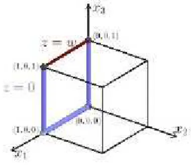
Figura 2 – The situation in Theorem 2.1.1
Thanks to the compatibility condition (2.3), we can argue as in (GUERREROet al., 2012) and check that
z∈C2([δ,1−δ]×[δ,1]×[0,T]) ∀δ >0.
inC0([δ,1−δ]×[δ,1]×[0,T])such that
z(x1,x3,t) =c(0)t+βδ(x1,x3,t)t2
∂xiz(x1,x3,t) =γδi(x1,x3,t)t2, i∈ {1,3}
∂tz(x1,x3,t) =c(0) +λδ(x1,x3,t)t
∂xi,x2 jz(x1,x3,t) =µδi j(x1,x3,t)t, i,j∈ {1,3}.
(2.4)
LetG andI be given by
G ={(x1,x2,x3):x2∈R, (x1,x3)∈(0,1)2},
I = ({0,1} ×R×(0,1))∪((0,1)×R× {0}).
Now, we introduce the functionsU andq, withU(x,t):= (0,z(x1,x3,t),0)andq:=
−c(t)x2. Note that the couple(U,q)satisfies
Ut−∆U+∇q=0 in G ×(0,T)
∇·U =0 in G ×(0,T)
U(x,t) =0 on I×(0,T)
U(x,0) =0 in G.
Later, we will look for a solution to the Navier-Stokes system of the form
u=N2U+y+ξ(t)W,
whereNis a large constant,yis the solution to a transport equation,W solves a Stokes system andξ ∈C2[0,2/N]is a cut-off function.
2.2.1.1 Transport equation
For an arbitrary initial condition y0 ∈V0(Ω)∩C01(Ω) extended by zero on G we
consider the system
yt+N2(U·∇)y+N2(y·∇)U=0 in Q2/N
y(x,t) =0 on Σ2/N
y(x,0) =y0(x) in Ω.
(2.5)
Here, we have used the notation
Let us denote byCδ the maximum of the norms of the functionsβδ,γδi,λδ andµδi j
inC0([δ,1−δ]×[δ,1]×[0,T]). We will look for a particular estimate fory, with an explicit
dependence onNthat is satisfied whenN is large enough. This is given in the following lemma: Lemma 2.2.1 Let y0∈C01(Ω)∩V0(Ω). For each smallδ >0, there exists Nδ =N(δ)such that,
for any N ≥Nδ, there exist a solution y to (2.5) and a positive constant Kδ (independent of N),
with the following properties:
kykC1(Q
2/N)≤Kδky0kC1(Ω) (2.6) and
y(x,t) =0 ∀(x,t)∈Ω×(1/N,2/N). (2.7)
Proof: Let us consider the Banach space
Y ={y∈C1(Q2/N):y(x,0) =y0(x)}. and the mappingΛ:Y 7→Y, given by
Λ(y)(x,t):=y0(x−N2Z(x,t))−N2
Z t
0(y·∇)U(x−N
2Z(x,s),s)ds,
Z(x,t):=
0,Z t
0 z(x1,x3,s)ds,0
.
Let us assume that suppy0⊂(δ,1−δ)3. It is easy to see that here existsNδ such
that, for anyN≥Nδ, we can applBanach’s Fixed-Point TheoremtoΛand deduce the existence and uniqueness of a solution to (2.5).
Let us puty0= (y0,1,y0,2,y0,3)andU = (U1,U2,U3). Then, we have
y1(x,t) =y0,1(x−N2Z(x,t)),
y2(x,t) =y0,2(x−N2Z(x,t))−N2
Z t
0 y·∇U2(x−N
2Z(s,x),s)ds,
y3(x,t) =y0,3(x−N2Z(x,t)).
From these identities, it is easy to check that, forN large enough, one has: kykC0(Q
2/N)≤Cky0kC0(Ω) k∇y1kC0(Q
2/N)≤Ck∇y0,1kC0(Ω) k∇y3kC0(Q
2/N)≤Ck∇y0,3kC0(Ω).
On the other hand, we also have k∇y2kC0(Q
2/N) ≤ 7k∇y0,2kC0(Ω)+Cδky0kC0(Ω)
+ 3Cδ
N k∇ykC0(Q2/N)+15 C2δ
N2k∇ykC0(Q2/N).
(2.9)
From (2.8) and (2.9), the inequality (2.6) holds (forN large enough). On the other hand, arguing as in the proof of Lemma 3 of (GUERREROet al., 2012) (see p. 693–695), we deduce (2.7).
This ends the proof.
2.2.1.2 The solution to a Stokes system with∇·W =−∇·y
Consider the following Stokes problem:
Wt−∆W+∇r=0, in Q2/N
∇·W =−∇·y, in Q2/N W(x,t) =0, on Σ2/N
W(x,0) =0, in Ω
W(x,t)→0 as|x2| →+∞.
(2.10)
The following result holds:
Proposition 2.2.1 Let W be the solution to(2.10). Then, for any p∈(1,+∞), there exists C (independent of N) such that
kWkLp(Q
2/N)≤C(p)N −1/p
ky0kC3(Ω). (2.11)
Furthermore, there exists a positive constant C>0(again independent of N) such that
kWkC0([0,2/N];L2(G))+k∂x2WkC0([0,2/N];L2(G))
+k∂x3WkC0([0,2/N];L2(G)) ≤CN−1/4.
(2.12)
The proof is given in (GUERREROet al., 2012) (see Proposition 1, p. 696).
2.2.2 Boussinesq system
Let us first introduce the functionsz2=z2(x1,t),z3=z3(x1,t)andΘ=Θ(x1,t)as
follows. First,z2is the solution to the system
∂tz2−∂x21x1z2=c(t) in (0,1)×(0,T)
z2(0,t) =0, z2(1,t) =w2(t) on (0,T)
z2(x1,0) =0 in (0,1),
(2.13)
wherec∈C2([0,T])is a positive function andw2is a nonnegative function satisfying
w2(t)∈C∞[0,T], w2(0) =0, w′2(0) =c(0), w2′′(0) =c′(0). Then,(z3,Θ)solves
∂tz3−∂x21x1z3=c(t) +Θ(x1,t) in (0,1)×(0,T) ∂tΘ−∂x21x1Θ=0 in (0,1)×(0,T)
z3(0,t) =0, z3(1,t) =w3(t) on (0,T) Θ(0,t) =0, Θ(1,t) =m(t) on (0,T)
z3(x1,0) =0, Θ(x1,0) =0 in (0,1).
(2.14)
with
w3∈C∞[0,T], w3(0) =0, w′3(0) =c(0), w3′′(0) =c′(0),
m∈C∞[0,T], m(0) =m′(0) =m′′(0) =0.
Proposition 2.2.2 Under the above assumptions on w2and c, there exist a unique solution to
(2.13)with
z2∈L2(0,T;H1(0,1))∩L∞((0,1)×(0,T)), ∂tz2∈L2(0,T;H−1(0,1)).
Furthermore, for all smallδ >0, we have z2∈C2([δ,1]×[0,T])and there exist functionsβ2,δ,
γ2,δ, µ2,δ andλ2,δ such that
(i) z2(x1,t) =c(0)t+β2,δ(x1,t)t2,|β2,δ| ≤Cδ,
(ii) ∂x1z2(x1,t) =γ2,δ(x1,t)t2,|γ2,δ| ≤Cδ,
(iii) ∂tz2(x1,t) =c(0) +µ2,δ(x1,t)t,|µ2,δ| ≤Cδ,
(iv) ∂x21x1z2(x1,t) =λ2,δ(x1,t)t,|λ2,δ| ≤Cδ.
The proof is not difficult. For instance, let us see how(i)can be proved. We simply write that
z2(x,t) = z2(x1,0) +
Z t
0 ∂tz2(x1,s)ds = ∂tz2(x,0)t+
Z t
0 ∂tz2(x1,s)ds−∂tz2(x1,0)t
where we have used the notation
β2,δ(x1,t):=
1 t2
Z t
0∂tz2(x1,s)ds−
1
t∂tz2(x1,0)
= (∂tz2(x,t˜)−∂tz2(x1,0))t−1 for some 0<t˜<t.
The proof of(ii),(iii)and(iv)follows through analogous computations.
A similar result can be established for the solution(z3,Θ)to (2.14):
Proposition 2.2.3 Under the above assumptions on c, w2, w3 and m, there exists a unique
solution(z3,Θ)to(2.14)with
z3∈L2(0,T;H1(0,1))∩L∞((0,1)×(0,T)),z3,t∈L2(0,T;H−1(0,1)),
Θ∈L2(0,T;H1(0,1))∩L∞((0,1)×(0,T)),Θt∈L2(0,T;H−1(0,1)).
Furthermore„ for all small δ >0, we have that z3,Θ∈C2([δ,1]×[0,T])2 and there exist
functionsβ3,δ,γ3,δ,µ3,δ,λ3,δ,β,γ andµ such that
(i) z3(x1,t) =c(0)t+β3,δ(x1,t)t2andΘ(x1,t) =β(x1,t)t2, with|β|,|β3,δ| ≤Cδ,
(ii) ∂x1z2(x1,t) =γ3,δ(x1,t)t2and∂x1Θ(x1,t) =γ(x1,t)t2, with|γ|,|γ3,δ| ≤Cδ,
(iii) ∂tz2(x1,t) =c(0)+µ3,δ(x1,t)t and∂tΘ(x1,t) =∂x21x1Θ(x1,t) =µ(x1,t)t, with|µ|,|µ3,δ| ≤
Cδ,
(iv) ∂x21x1z2(x1,t) =λ3,δ(x1,t)t, with|λ3,δ| ≤Cδ.
Now, consider the functionsU(x,t) = (0,z2(x1,t),z3(x1,t)),Θ=Θ(x1,t)as before
and q(x,t) =−(x2+x3)c(t). Observe that(U,q,Θ)solves the following Boussinesq problem:
Ut−∆U+ (u·∇)U+∇q=Θe3, in G ×(0,T)
∇·U =0 in G ×(0,T)
Θt−∆Θ+U·∇Θ=0 in G ×(0,T)
U(0,x2,x3,t) =0, Θ(0,x2,x3,t) =0 on R2×(0,T)
U(x,0) =0, Θ(x,0) =0 in G.
In the proof of Theorem 2.1.3, the construction of the solution to (2.2) is divided into four steps. In one of them,(u,θ,p)is written in the form
u(x,t) =N2U(x,t) +y(x,t)−ξ(t)W(x,t), (x,t)∈Ω×(T1,T2) θ(x,t) =N2Θ(x,t) +h(x,t), (x,t)∈Ω×(T1,T2)
p(x,t) =N2q(x,t) +ξ(t)r(x,t), (x,t)∈Ω×(T1,T2),
where(y,h)is the solution to a transport equation andW is the solution to a linear Stokes system. In the next two paragraphs, we construct(y,h)andW and we prove some estimates.
For anyδ >0, we define
C0δ(G×[0,2/N])4:={(y,h)∈C0(G×[0,2/N])4:y=0,h=0 forx1∈[0,δ]}.
2.2.2.1 Another transport system
For an arbitrary initial condition extended by zero onG and for someN>0 large enough (to be defined precisely later), we solve the following null controllability problem for the transport equation
yt+N2(U·∇)y+N2(y·∇)U =he3 in Q2/N ht+N2U·∇h+N2y·∇Θ=0 in Q2/N
y(0,x2,x3,t) =0, h(0,x2,x3,t) =0 on R2×(0,2/N)
y(x,0) =y0(x), h(x,0) =h0(x) in G,
(2.16)
whereQ2/N =G×(0,2/N).
Lemma 2.2.2 Let us assume that(y0,h0)∈(C10(Ω)∩V0(Ω))×C01(Ω). For eachδ >0, there
exists N0(δ)such that, for any N ≥N0(δ), there exist a solution(y,h)to(2.16)and a positive constant C(δ)(independent of N) such that(y,h)∈Cδ0(G ×[0,2/N]),
kykC1
δ(Q2/N)+khkCδ1(Q2/N)≤C(δ)k(y0,h0)kC1(Ω), (2.17)
kytkC1
δ(Q2/N)+khtkCδ1(Q2/N)≤C(δ)k(y0,h0)kC1(Ω) (2.18) and
y(x,t) =0, h(x,t) =0 ∀(x,t)∈Ω×(1/N,2/N).
2.3 Proof of Theorem 2.1.3
Let us first prove the controllability result in Theorem 2.1.3.
As mentioned above, we will closely follow the arguments in the proof of Theorem 1 in (GUERREROet al., 2012). As there, we consider several steps, each one related to a time subinterval.
• FIRST STEP: We know that there exists at least one weak solution(u,p,θ)to the
problem
ut−∆u+ (u·∇)u+∇p=θe3+f, ∇·u=0 in Q
θt−∆θ+u·∇θ =g in Q
u=0, θ =0 on ∂Ω×(0,T)
(u(x,0),θ(x,0)) = (u0,θ0) in Ω,
with
u∈L2(0,T;V0(Ω))∩L∞(0,T;H(Ω)), θ∈L2(0,T;H01(Ω))∩L∞(0,T;L2(Ω)).
Let ˜T1∈(T−δ0,T) be such that (u˜1,θ˜1):= (u(·,T˜1),θ(·,T˜1))∈V0(Ω)×H01(Ω)
and
kfkL2(T−δ,T;V′
0(Ω))+kgkL2(T−δ,T;H−1(Ω)) ≤ ε
5.
For any smallη>0 with ˜T1+η<T, there exists a unique strong solution(u,p,θ)to the
Bous-sinesq problem inΩ×((T˜1,T˜1+η), with(u(·,T˜1),θ(·,T˜1)) = (u˜1,θ˜1)(see for instance
(CONS-TANTIN; FOIAS, 1988)) and there exist manyT1∈(T˜1,T˜1+η)with
(u(·,T1),θ(·,T1))∈(H2(Ω)3∩V0(Ω))×(H2(Ω)∩H01(Ω)).
On the interval(0,T1)we do not exert any control and we take
uε :=u, pε :=p, fε := f, θε :=θ, gε :=g.
• SECOND STEP: Let us write(u1,θ1):= (u(·,T1),θ(·,T1))and let us takeu1,α ∈
V0(Ω)∩C0∞(Ω)3andθ1,α ∈C0∞(Ω)with
and
ku1,αkV0(Ω)+kθ1,αkH1
0(Ω)≤2(ku1kV0(Ω)+kθ1kH01(Ω)).
LetT2∈(T1,T)be a time; its precise value will be given below. We introduce now (uε,pε,θε)in(T1,T2), with
uε=
t−T1
T2−T1u1,α+
T2−t
T2−T1u1, pε =0, fε=
Luε−θεe3,
θε =
t−T1
T2−T1θ1,α+
T2−t
T2−T1θ1, gε =
Mεθε,
where
Luε := ∂tuε−∆uε+ (uε·∇)uε Mεθε := ∂tθε−∆θε+uε·∇θε.
It is then clear that
(uε(·,T1),θε(·,T1)) = (u1,θ1), (uε(·,T2),θε(·,T2)) = (u1,α,θ1,α), ∇·uε=0
and the couple(fε,gε)satisfies(fε,gε)∈L2(Q)3×L2(Q),
kfεkL2(T1,T2;V′
0(Ω))≤
C √
T2−T1ku1,α−u1kV0(Ω) +C√T2−T1
ku1kH1
0(Ω)3+ku1k 2
H01(Ω)3+kθ1kH01(Ω)
and
kgεkL2(T1,T2;H−1(Ω))≤ √ C
T2−T1kθ1,α−θ1kH01(Ω) +C√T2−T1
kθ1kH1
0(Ω)+kθ1kH01(Ω)ku1kH01(Ω)3
.
Accordingly, we can choose firstT2close enough ofT1and thenα small enough to have
kfεkL2(T
1,T2;V0′(Ω))+kgεkL2(T1,T2;H−1(Ω))≤ ε
5.
• THIRD STEP: Let us set
u2:=uε(·,T2)∈V0(Ω)∩C0∞(Ω)3, θ2:=θε(·,T2)∈C0∞(Ω).
We will work in the interval(T2,T2+2/N), whereN≥N(δ),N(δ)is furnished by Lemma 2.2.2
In this step, we will take
uε(x,t) = N2U˜(x,t) +y˜(x,t)−ξ(t−T2)W˜(x,t),
pε(x,t) = −N2(x2+x3)c(t−T2) +r˜(x,t), θε(x,t) = N2Θ˜(x,t) +h˜(x,t)
and
fε = −∆y˜+((y˜−W˜)·∇)(y˜−W˜)−N2(U˜ ·∇)W˜ −N2(W˜ ·∇)U˜−ξtW˜, gε = −∆h˜+(y˜−W˜)·∇h˜−N2W˜ ·∇Θ˜.
Here, ˜U, ˜Θ, etc. are respectivelyU, Θ, etc. written at timet−T2, (U,θ) is the
solution to (2.15),(y,h)is the solution to (2.16) with initial data(y0,h0) = (u2,θ2),(W,r)is the
solution to (2.10) andξ ∈C2([0,2/N])is a cut-off function satisfying
ξ(t) =1 in (0,1/N) and ξ(t) =0 in a neighborhood of 2/N.
From the properties of(y,h)deduced in Lemma 2.2.2 and the definitions ofU andW, we have the following:
(uε,θε)(x,T2+2/N)≡N2(U,Θ)(x1,2/N), ∇·uε ≡0
and
uε(0,x2,x3,t) =0, θε(0,x2,x3,t) =0 in (0,1)2×(T2,T2+2/N).
Let us check that, forNlarge enough, we have
kfεkL2(T2,T2+2/N;V′
0(Ω))+kgεkL2(T2,T2+2/N;H−1(Ω)) ≤
ε
5. First, note that Lemma 2.2.2 yields
k∆y˜kL2(T
2,T2+2/N;V0′(Ω))+k∆h˜kL2(T2,T2+2/N;H−1(Ω))≤
C N1/2. Let us decomposeΩin two sets
Recall that∇·y=∇·W in Q2/N andy=0 in Ω1. Consequently, kN2(W˜ ·∇)U˜kV′
0(Ω)= sup
β∈V0(Ω),kβkV
0(Ω)=1
Z
Ω1
N2(W˜ ·∇)U˜βdx
+ sup
β∈V0(Ω),kβkV0(Ω)=1
Z
Ω2N 2(W˜
·∇)U˜βdx
=− sup
β∈V0(Ω),kβkV0(Ω)=1
Z
Ω1N 2W˜
·∇βU dx˜
+ sup
β∈V0(Ω),kβkV0(Ω)=1
Z
Ω2N 2(W˜
·∇)U˜βdx.
The first term is bounded byCkNW˜kL2(Ω)kNU˜kL∞(Ω). On the other hand, Z
Ω2N
2(W˜ ·∇)U˜βdx≤ kN∇U˜kL
∞((δ/2,1)×R2)kNW˜kL2(Ω).
Thanks to Propositions 2.2.2 and 2.2.3, there existsC(δ)>0 such that
kN∇U˜kL∞(T
2,T2+2/N;L∞((δ/2,1)×R2)≤C. Therefore, we see from (2.12) that
kN2(W˜ ·∇)U˜kLr(T
2,T2+2/N;V0′(Ω)) ≤C
Z T2+2/N
T2 k
NWkrL2(Ω)dt 1/r
≤CN3/4−1/r.
Similarly, the following estimate can be obtained: kN2W˜ ·∇ΘkLr(T
2,T2+2/N;H−1(Ω))+kN2(U˜·∇)W˜kLr(T
2,T2+2/N;V0′(Ω))
≤CN3/4−1/r.
Next, using (2.11), we deduce that
kξtWkLr(T
2,T2+2/N;L2(Ω)3)≤kWkLr(T
2,T2+2/N;L2(Ω))≤C(r)N−1/rku2kC1(Ω). Also,
k((y˜−W˜)·∇)(y˜−W˜ )kL2(T2,T2+2/N;V′
0)≤Cky˜−W˜k 2
L4(T2,T2+2/N;L4(Ω)3)
and, from Lemmas 2.2.2 and (2.11), this quantity goes to zero asN→+∞. Similarly,
k(y˜−W˜)·∇hkL2(T2,T2+2/N;H−1)
≤Ckh˜kL4(T2,T2+2/N;L∞(Ω))ky˜−W˜kL4(T2,T2+2/N;L2(Ω)3)→0
• FOURTH STEP:
Finally, we set T3:= T2+2/N and we work in the interval (T3,T). Note that (uε,pε,θε)arrives att=T3with the following structure:
uε(x,T3) = 0,N2z2(x1,2/N),N2z3(x1,2/N), θε(x,T3) = N2(∂tz3+∆z3)(x1,2/N).
The second component ofuεcan be driven to zero at timet=T by solving a standard
null controllability problem for a linear heat equation. On the other hand, the third component ofuεandθε can be driven to zero by solving a (less standard) null controllability problem for a
system of two coupled 1D parabolic PDEs.
Indeed, let us take fε =0 andgε =0 in(T3,T). It is well-known that there exists ρ ∈L∞(0,T−T3)such that the solution to
∂tz−∂x21x1z=0, in (0,1)×(0,T−T3)
z(0,t) =0, z(1,t) =ρ(t), on (0,T−T3)
z(x1,0) =N2z2(x1,2/N) in (0,1)
satisfies
z(x1,T−T3) =0 in (0,1).
On the other hand, it is proved in (FERNÁNDEZ-CARA et al., 2010) that, if A∈L(R2)andB∈R2,µ1 and µ2are the eigenvalues ofA, rank[B|AB] =2,(T/π)(µ1−µ2) is not a integer of the form 4(m+1)or 2m+1 withm≥1 andy0∈H−1(0,1)2, there exists a controlv∈L2(0,T−T3)such that the associated solution to the system
∂ty−∂x21x1y=Ay, in (0,1)×(0,T−T3)
y(0,t) =0, y(1,t) =Bv, on (0,T−T3)
y(x1,0) =y0(x1) in (0,1)
(2.19)
satisfies
y(x1,T−T3) =0 in (0,1). (2.20)
Then, it suffices to defineuε andθε in(T3,T)as follows: