Instituto de Ciências Biológicas Programa de Pós-Graduação em Ecologia
ALMIR PICANÇO DE FIGUEIREDO
Novos métodos em Ecologia de Estradas: Correção da
heterogeneidade espacial na análise de agregação de
atropelamentos de fauna e definição da suficiência
amostral
atropelamentos de fauna e definição da suficiência
amostral
Almir Picanço de Figueiredo
Orientadora: Ludmilla M. S. Aguiar
BRASÍLIA 2017
Se avexe não
Amanhã pode acontecer tudo
Inclusive nada
Se avexe não
A lagarta rasteja até o dia
Em que cria asas
Se avexe não
Toda caminhada começa
No primeiro passo
A natureza não tem pressa
Segue seu compasso
Inexoravelmente chega lá
Se avexe não
Observe quem vai subindo a ladeira
Seja princesa ou seja lavadeira
Pra ir mais alto vai ter que suar
Agradeço sempre aos meus pais Ademir e Romana por tudo, por formarem meu caráter e por me fazer capaz de me desafiar e superar meus desafios
Agradeço aos meus irmãos Ademir, Marcy e Neto pelo amor, pelo apoio que sempre nos demos, por terem me ajudado a crescer, até hoje inclusive.
Aos meus professores, da Escolinha Pingo de Mel, da Escola Tenente Rêgo Barros, do IB-USP e do PPG de Ecologia da UnB.. Em nome deles cito os professores Samuel e Davi Eduardo que me inspiraram a escolher o estudo da vida como profissão.
Ao pessoal do Rodofauna, Rodrigo, Leandro, Felipe, Marina, Javier, Cecília e Carol, pelo grande apoio nas coletas de campo, pelas boas conversas durante as coletas e pelos debates durante as análises de dados.
Aos amigos da Coordenação de Fauna do Ibram, Ana Nira, Elenize, João Bosco, Thiago, Marina, Rodrigo (de novo) e Fernanda, por formarem o melhor setor para se trabalhar e por me ajudarem a aguentar o peso no mestrado, quebrando vários galhos no trabalho.
Aos amigos da Ecologia da Unb, Marcela, Jéssica, Elba, Marília, Sara, Danilo, Laura, Nayara, Dariane, Camila, Carla, Bárbara, Tarcísio, Silvia, Marcos, Vicente e os que esqueci de citar mas que em diversos momentos deste 02 anos e meio me deram muito apoio, seja com a experiência ou com a juventude me inspiraram a persistir.
A todos os professores do Programa de Pós-Graduação em Ecologia da UnB por todo o aprendizado que obtive e por terem me dado tempo e solidariedade quando eu precisei.
À professora Ludmilla, por ter me aceitado como aluno e ter confiado em mim desde o início mesmo com o oceano Atlântico de distância entre nós. E por terminar todas as nossas conversas deixando sempre claro que confiava em mim.
Ao Ibram por manter um programa de monitoramento de fauna atropelada há tantos anos, sendo o ÚNICO órgão ambiental do Brasil a ter um programa permanente deste tema, mostrando a consciência quanto à relevância do impacto das rodovias sobre a fauna.
LISTA DE FIGURAS ... viii
LISTA DE TABELAS ... x
RESUMO GERAL ... 1
Palavras chave ... 1
KEY WORDS ... 2
INTRODUÇÃO GERAL ... 3
Agregação espacial na Ecologia de Estradas ... 4
O problema da não homogeneidade na estatística espacial de pontos ... 8
Suficiência amostral em Ecologia de Estradas ... 10
CAPÍTULO 01 - DEALING WITH INHOMOGENEITIES IN ROAD ECOLOGY: A NEW HOTSPOT ANALYSIS ... 17
ABSTRACT ... 18
2. MATERIAL AND METHODS ... 22
2.1. Simulated study ... 22
2.2. Real data study ... 26
3. RESULTS ... 29
3.1 Simulated study ... 29
3.1 Real data study ... 34
4. DISCUSSION ... 37
6. ACKNOWLEDGEMENTS... 41
7 BIBLIOGRAPHY ... 42
CAPÍTULO 02 – DEFINIÇÃO DA CURVA DE PRECISÃO PARA ANÁLISE DA SUFICIÊNCIA AMOSTRAL EM ECOLOGIA DE ESTRADAS ... 48
RESUMO... 48
ABSTRACT ... 49
INTRODUÇÃO ... 51
MÉTODOS ... 53
DISCUSSÃO ... 64
CONCLUSÃO ... 67
REFERÊNCIAS ... 68
CONSIDERAÇÕES FINAIS ... 72 ANEXO I - SCRIPTS DA PROGRAMAÇÃO REALIZADA PARA A DISSERTAÇÃO
INTRODUÇÃO GERAL
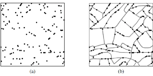
Figura 1 Diferença entre distribuição de eventos sobre um espaço Euclidiano (a) e sobre ou ao longo de uma rede linear (b). Fonte: Okabe & Sugihara (2012) ... 5
CAPÍTULO 01 - DEALING WITH INHOMOGENEITIES IN ROAD ECOLOGY: A NEW HOTSPOT ANALISYS
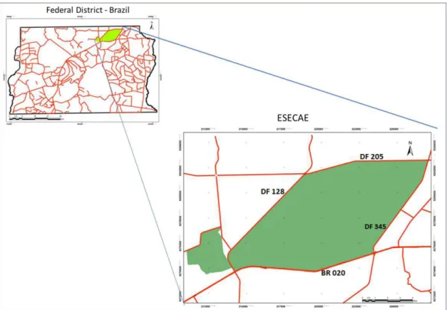
Figure 1. The large green area is the Águas Emendadas Ecological Station – ESECAE, in Brasília, Federal District of Brazil. ... 27 Figure 2. All graphs show the effects of changes in density and in distribution noise
types on the three methods results. Graphs A and B show the results considering all scales of analysis and graphs C and D show those considering only the most efficient analyses for each method, that is, a radius of 200 m for the Hotspot 2D formula and Malo’s method and a radius of 200 m with a window of 2,800 m for the Windowned method. For all graphs, the red triangles, green squares and black circles represent the Hotspot 2D formula, Malo’s method and the Windowned method, respectively ... 32 Figure 3. Results of the hotspot analysis using the Windowned methodology (graph A), Hotspot 2D (graph B) and Malo’s method (graph C). ... 34 Figure 4. The columns represent the results obtained using the Windowned method, Hotspot 2D and Malo’s method, respectively. Each of the lines represents the removal of a highway from the study area, and in the downward direction, we have the removal of BR-020, followed by DF-345, DF-205 and finally DF-128. The triangles represent original hotspots that were not classified as such by the analysis with the removal of a highway, and the circles are the points not originally identified as hotspotsbut have been classified as such in the analyses ... 36
CAPÍTULO 01 - DEALING WITH INHOMOGENEITIES IN ROAD ECOLOGY: A NEW HOTSPOT ANALISYS
Table 1 Number of hotspots that ‘appeared’ - False Positive Hotspot -and ‘disappeared’ - False Negative Hotspot - due to the withdrawal of a highway in the analysis of hotspots. ... 35
CAPÍTULO 02 – DEFINIÇÃO DA CURVA DE PRECISÃO PARA ANÁLISE DA SUFICIÊNCIA AMOSTRAL EM ECOLOGIA DE ESTRADAS
Tabela 1 Padrões de divisões do total de dados para criação dos subconjuntos ... 56 Tabela 2 Conjuntos de dados utilizados para avaliar a construção da curva de precisão
de tempos diferentes da coleta de dados ... 56 Tabela 3 Estimativa da precisão atual da indicação de hotspots de atropelamento de
RESUMO GERAL
O atropelamento de fauna é considerado por diversos autores como a principal causa direta de morte de animais na natureza. No entanto, as intervenções necessárias para mitigar este efeito negativo das rodovias são geralmente onerosas e por isso é preciso ter confiabilidade na proposição de locais para as mesmas. As análises de agregação de atropelamento usadas em Ecologia de Estrada não corrigem o efeito da heterogeneidade de densidade de primeira ordem gerando uma autocorrelação espacial entre os atropelamentos maior do que a real. O primeiro capítulo desta dissertação apresenta um método de correção, denominado Windowned Method, o qual pondera os resultados obtidos em um raio de análise por uma janela de observação com menor heterogeneidade que a área total de estudo. O método proposto apresentou menores taxas de erro de classificação de hotspot e sofreu menos influência da heterogeneidade de distribuição dos eventos, quando comparado com dois outros métodos usados em Ecologia de Estradas. Esta dissertação também abordou a deficiência de uma análise de suficiência amostral para estudos de Ecologia de Estradas. No segundo capítulo desta dissertação foi verificado que existe relação positiva entre a precisão de classificação de hotspot e o tamanho da amostra. Por meio de simulações por reamostragem Bootstrap e por extrapolações utilizando Regressão Quantílica, esta relação foi utilizada para construção de uma Curva de Precisão com a qual é possível identificar o tamanho da amostra desejada para se atingir um grau de precisão determinado pelo pesquisador. Com este método a suficiência amostral pode ser determinada pelo acúmulo de registro permitindo protocolos de coletas diversos, permitindo ao pesquisador variar a velocidade de busca por carcaças e frequência de campanhas de coletas, conforme sua conveniência.
PALAVRAS CHAVE
Agregação Virtual, Atropelamento, Heterogeneidade, Suficiência Amostral
ABSTRACT
Roadkills is considered by several authors as the main direct cause of death of animals in nature. However, the interventions needed to mitigate this negative effect of the highways are usually onerous and therefore it is necessary to have reliability in proposing sites for them. The roadkill aggregation analyzes used in Road Ecology do not correct the effect of first order density heterogeneity by generating spatial autocorrelation between events greater than the actual is. The first chapter of this dissertation presents a method of correction, called Windowned Method, which weighs the results obtained in a radius of analysis by an observation window with less heterogeneity than the total area of study. The proposed method presented lower hotspot classification error rates and was less influenced by the heterogeneity of event distribution when compared to two other methods used in Road Ecology. This dissertation also addressed the deficiency of a sample adequacy analysis for Road Ecology studies. In the second chapter of this dissertation it was verified that there is a positive relationship between the hotspot classification accuracy and the sample size. By means of Bootstrap resampling simulations and extrapolations using Quantile Regression, this relation was used to construct a Precision Curve with which it is possible to identify the desired sample size to reach a degree of precision determined by the researcher. With this method the sampling sufficiency can be determined by the accumulation of record allowing diverse collection protocols, it permits researchers to vary both the speed of carcasses search as the frequency of collections campaigns, according to their convenience.
KEY WORDS
INTRODUÇÃO GERAL
O termo "ecologia da estrada" foi proposto por Richard T. T. Forman em 1998 (Coffin 2007). O termo se refere a um assunto de investigação ecológica com base na evidência de que as estradas exercem efeitos sobre componentes, processos e estruturas do ecossistema, e que as causas desses efeitos são tanto relacionadas à engenharia quanto ao planejamento do uso da terra e à política de transportes (Coffin 2007). Estes efeitos incluem a degradação do habitat (Jaeger & Fahrig 2004, Taylor & Goldingay 2012), poluição química e sonora, erosão e sedimentação dos corpos hídricos (Trombulak & Frissell 2000), mudança no comportamento de algumas espécies (Blackwell et al. 2014, Lima et al. 2014, DeVault et al. 2015) e a dispersão de espécies exóticas (Trombulak & Frissell 2000). No entanto, a colisão com automóveis é a principal fonte de mortalidade direta em algumas populações animais (Trombulak & Frissell 2000, Gibbs & Shriver 2002, Glista et al. 2008).
As estratégias para mitigação do impacto dos atropelamentos de fauna são normalmente muito caras (Huijser et al. 2009, Mountrakis & Gunson 2009, Santos et al. 2015), não sendo viável a implantação ao longo de toda rodovia estudada. Por isso, para identificar trechos da rodovia onde existe maior probabilidade de sua ocorrência e dessa forma obter maior benefício para as populações de fauna impactadas, a partir da aplicação dos recursos disponíveis, é necessário conhecer o padrão espacial da distribuição de atropelamentos (Huijser et al. 2009, Polak et al. 2014, Santos et al. 2015).
al. 2014, Snow et al. 2014), e o segundo grupo por aqueles que visam identificar áreas
geográficas com incidência de atropelamento maior do que o esperado ao acaso, ou seja, os hotspots de atropelamento (Clevenger et al. 2003, Ramp et al. 2005, Gomes et al. 2008, Seo et al. 2013, Skórka et al. 2015).
Agregação espacial na Ecologia de Estradas
O primeiro trabalho que demonstrou que atropelamentos de fauna não ocorrem aleatoriamente foi realizado por Puglisi et al. (1974). Nesse trabalho foi observado que a quantidade de atropelamentos de cervídeos era menor em locais onde as cercas no entorno das rodovias estavam a mais de 23 metros de áreas arborizadas. Porém, a presença de vegetação somente tinha relação com atropelamentos nos locais onde não havia cercas. Entretanto, o primeiro trabalho a descrever e medir o padrão espacial de agregação ocorreu em 2003, no qual os autores apresentaram uma adaptação da função K de Ripley (Ripley 1976) para eventos pontuais que ocorrem sobre rodovias (Clevenger et al. 2003). A adaptação proposta por Clevenger et al. (2003) ocorreu de forma independente e praticamente simultânea ao trabalho de Okabe & Yamada (2001), que propôs adaptação semelhante para eventos denominados por eles de eventos sobre ou ao longo de redes lineares ou eventos em rede (network events).
Figura 1 Diferença entre distribuição de eventos sobre um espaço Euclidiano (a) e sobre ou ao longo de uma rede linear (b). Fonte: Okabe & Sugihara (2012)
A análise da não aleatoriedade da agregação de eventos compara os resultados observados com aqueles obtidos por aleatorizações e estes eventos simulados podem ocorrer em qualquer localização do espaço euclidiano em questão. Assim sendo, ao se comparar os eventos que somente ocorreram sobre determinadas linhas com os aleatorizados sobre todo o plano, o valor de K não representaria a realidade de dependência entre os eventos (Okabe & Sugihara, 2012). A correção deste problema é o uso do caminho mais curto sobre a rede, ao invés de distância Euclidiana, para medir a distância entre dois eventos na aplicação da função K (Okabe & Yamada, 2001). Esta correção foi denominada Função K para Rede (Network K Function) – fórmula (1) – e os autores denominaram a função tradicionalmente utilizada como Função K planar (Planar K Function) para distinguir ambas fórmulas.
𝐾̂𝐿(𝑟) = 𝑛(𝑛 − 1) ∑ ∑ 1{𝑑𝐿 𝐿(𝑥𝑖, 𝑥𝑗) ≤ 𝑟} 𝑗≠𝑖
(1)
𝑛
Onde L significa o comprimento total da rede linear estudada, r é o raio da circunferência de análises e dL(xi,xj) significa a menor distância entre i e j, que tem valor de 1 ser for menor ou igual ao raio r e valor 0 se for maior.
Um outro estudo comparou os resultados obtidos com a aplicação das funções K para redes e planar sobre o padrão de acidentes de trânsito (Yamada & Thill 2004). Além disso, incluíram nesta comparação uma metodologia intermediária: o uso da distância euclidiana entre os eventos, conforme a função planar, comparando com eventos aleatorizados sobre a rede em análise, conforme a função K para redes. Neste estudo, os autores identificaram uma superestimativa de dependência entre eventos tanto para metodologia intermediária, como para a função K planar - esta última apresentando maior diferença.
Steenberghen et al.(2010) denominaram como redes bi-dimensionais (2D Network) aquelas redes cujos movimentos não estão restritos aos trechos lineares da rede. Para estes casos Okabe & Sugihara (2012) ressaltam que mesmo os eventos ocorrendo sobre, ou ao longo de redes, o uso do caminho mais curto sobre a rede não é o mais adequado para medir a distância entre pares de eventos.
determinada distribuição de pontos difere de uma distribuição aleatória. Porém, não revela a localização das agregações dentro da distribuição (Steenberghen et al. 2010). Em Ecologia de Estrada, alguns autores usam essa função – adaptada por Okabe & Yamada (2001) e depois por Coelho et al.(2008) – como uma etapa anterior na identificação de pontos com taxas de acidentes superiores aos esperados, denominado hotspots de atropelamento (ex. Ramp et al. 2005, Mountrakis & Gunson 2009, Coelho
et al. 2012). A análise de Hotspot 2D, proposta por Coelho et al.(2012) é uma adaptação
da função K que usa janelas de varredura para testar se a intensidade dos pontos dentro de uma destas janelas é significativamente maior do que esperado ao acaso (Coelho et al. 2014).
Tanto a função K como a análise de Hotspot 2D testam a completa aleatoriedade espacial. Os testes de função K avaliam se os pontos exibem agregação ou dispersão, em vez de independência, enquanto a análise de Hotspot 2D assume que os pontos são independentes e testam se existem regiões com maior intensidade que o esperado (Coelho et al. 2014).
O método Malo, assim como o Hotspot 2D, compara a quantidade de registros em uma janela de análise contra o esperado por uma distribuição aleatória de Poisson. As diferenças entre os dois métodos são: 1) as janelas do método Malo não se sobrepõem, ao contrário das 'janelas deslizantes' usadas no Hotspot 2D; 2) O método Hotspot 2D usa o raio em torno de um ponto fixo e distância euclidiana para registrar
como regra de contagem, enquanto o método Malo usa distâncias de estrada; 3) O Hotspot 2D corrige os dados registrados pelos trechos rodoviários presentes no raio de
análise, o que não é necessário no método Malo, pois todos os trechos de análise possuem a mesma extensão rodoviária. Assim, a principal semelhança entre estes dois métodos é a utilização de um modelo nulo, baseado em distribuição de Poisson, para identificar quais trechos das rodovias apresentam valores superiores ao esperado, com base na completa aleatoriedade espacial dos eventos. Além disso, ambos os métodos consideram como premissa para suas aplicações a homogeneidade da distribuição dos eventos com padrões pontuais.
O problema da não homogeneidade na estatística espacial de pontos
A combinação destes efeitos gera seis (6) classes de distribuição (Wiegand & Moloney 2014). No entanto, esta dissertação abordará duas classificações, denominadas: “Processo pontual homogêneo com interações” e “Processo pontual heterogêneo de primeira ordem”. Um processo pontual homogêneo com interações é a
classe alvo da maioria das análises de padrões pontuais. Segundo esta distribuição, um ponto pode ocorrer em qualquer lugar na área de estudo com a mesma probabilidade (intensidade constante). Além disso, por esta distribuição, existe interação entre os eventos, e a regra de interação é a mesma em qualquer local da área de estudo (interação homogênea). Para estas análises, utiliza-se a distribuição de Poisson como modelo nulo. Já um processo pontual heterogêneo de primeira ordem também apresenta interação homogênea entre os eventos, mas nesse caso, os fatores externos exercem influência na intensidade de eventos. Ou seja, a probabilidade de ocorrência de um evento não é a mesma para diferentes locais da área de estudo (Wiegand & Moloney, 2014).
proposta por Okabe & Yamada (2001) precisa ser corrigida para distribuições não homogêneas de eventos. Dentro desse escopo, o capítulo 1 desta dissertação apresenta uma proposta de correção metodológica para o método Hotspot 2D com a utilização de janelas de observação, de forma que a densidade local seja ponderada pela densidade de uma vizinhança com maior homogeneidade do que toda a área de estudo. O referido capítulo está formatado como artigo científico submetido à apreciação para publicação.
Suficiência amostral em Ecologia de Estradas
Quando uma amostra é tomada de um universo amostral, não é possível saber se o estado de um atributo obtido coincide com o seu estado verdadeiro (Pillar 2004). Porém, quanto maior o tamanho da amostra, maior é a chance de obter novas amostras que indiquem as mesmas conclusões (Pillar 2004). O estado de um dado atributo obtido a partir da amostra evolui e atinge estabilidade a medida que o número de unidades amostrais na amostra aumenta. O incremento de unidades amostrais implica em alterações relativamente menores no valor do atributo considerado (Pillar 2004). Assim, o tamanho suficiente da amostra será aquele em que o atributo da amostra atinge estabilidade (Pillar 2004).
A curva "número de espécies versus número de unidades amostrais” é usada para indicar a suficiência de amostragem em ecologia de comunidades, mas quaisquer outros atributos, simples ou complexos (e.g., medidas de diversidade), poderiam também ser considerados nessas curvas (Pillar 2004). No entanto, em Ecologia de Estradas não se conhece a relação entre o tamanho da amostra e as respostas que se quer obter com a sua análise.
Duas importantes fontes de erro amostral nos estudos de ecologia de estradas são amplamente conhecidas na literatura especializada: o tempo em que a carcaça fica disponível nas rodovias para ser registrada (Slater 2002, Teixeira et al. 2013a), e a ineficiência de detecção das carcaças nas rodovias, intrínseco ao método de coleta utilizado (Teixeira et al. 2013a, Santos et al. 2016). Todos estes autores indicam a necessidade de se corrigir estatisticamente as taxas de atropelamento. Entretanto, não foram encontrados estudos que demonstrem o impacto da correção da taxa de atropelamento na distribuição espacial da ocorrência dos mesmos.
Referências
Ang Q.W., A. Baddeley & G. Nair (2012). Geometrically corrected second order analysis of events on a linear network, with applications to ecology and criminology. Scandinavian Journal of Statistics 39: 591–617.
Baddeley A.J., J. Møller & R. Waagepetersen (2000). Non and semi-parametric estimation of interaction in inhomogeneous point patterns. Statistica Neerlandica 54: 329–350.
Blackwell B.F., T.W. Seamans & T.L. Devault (2014). White-tailed deer response to vehicle approach : evidence of unclear and present danger. PLoS One 9: e109988.
doi:10.1371/journal.pone.0109988.
Clevenger A.P., B. Chruszcz & K.E. Gunson (2003). Spatial patterns and factors influencing small vertebrate fauna road-kill aggregations. Biological Conservation 109: 15–26.
Cochran W.G. (1977). SamplingTechniques. Third Edition. John Wiley and Sons Ltd. Coelho A.V.P., I.P. Coelho, F.Z. Teixeira & A. Kindel (2014). Siriema: road mortality
software. User´s guide. NERF/UFRGS, Porto Alegre, Brasil.
Coelho I.P., A. Kindel & A.V.P. Coelho (2008). Roadkills of vertebrate species on two highways through the Atlantic Forest Biosphere Reserve, southern Brazil. European Journal of Wildlife Research 54: 689–699.
Coelho I.P., F.Z. Teixeira, A.V.P. Coelho & A. Kindel (2012). Anuran road-kills neighboring a peri-urban reserve in the Atlantic Forest, Brazil. Journal of Environmental Management 112: 17–26.
Proceedings of Royal Society B, p. 282. http://dx.doi.org/10.1098/rspb.2014.2188. Forman R.T.T. & L.E. Alexander (1998). Roads and their major ecological effects.
Annual Review of Ecology and Systematics 29: 207–231.
Gibbs J.P. & W. G. Shriver (2002). Estimating the effects of road mortality on turtle populations. Conservation Biology 16: 1647–1652.
Glista D.J., T.L. DeVault & J.A. DeWoody (2008). Vertebrate road mortality predominantly impacts amphibians. Herpetological Conservation and Biology 3: 77–87.
Gomes L., C. Grilo, C. Silva & A. Mira (2008). Identification methods and deterministic factors of owl roadkill hotspot locations in mediterranean landscapes. Ecological Research 24: 355–370.
Grilo C., J.A. Bissonette & M. Santos-Reis (2009). Spatial–temporal patterns in mediterranean carnivore road casualties: consequences for mitigation. Biological Conservation 142: 301–313.
Grilo C., D. Reto, J. Filipe, F. Ascensão & E. Revilla (2014). Understanding the mechanisms behind road effects: linking occurrence with road mortality in owls. Animal Conservation 17: 555–564.
Grovenburg T.W., J.A. Jenks, K.L. Monteith, D.H. Galster, R.J. Schauer, W.W. Morlock & J. A. Delger (2008). Factors affecting road mortality of whitetailed deer in eastern South Dakota. Human-Wildlife Interactions 2: 48–59.
Huijser M. P., J. W. Duffield, A. P. Clevenger, R. J. Ament & P. T. McGowen (2009). Cost–benefit analyses of mitigation measures aimed at reducing collisions with large ungulates in the United States and Canada; a decision support tool. Ecology and Society 14(2): 15.
Conservation Biology 18: 1651–1657.
Lima S.L., B.F. Blackwell, T.L. Devault & E. Fernández-Juricic (2014). Animal reactions to oncoming vehicles : a conceptual review. Biological Reviews 10.1111/brv.12093.
Malo J.E., F. Suárez & A. Díez (2004). Can we mitigate animal–vehicle accidents using predictive models? Journal of Applied Ecology 41: 701–710.
Mountrakis G. & K. Gunson (2009). Multi-scale spatiotemporal analyses of moose– vehicle collisions: a case study in northern Vermont. International Journal of Geographical Information Science 23: 1389–1412.
Nielsen C.K., R.G. Anderson & M.D. Grund (2003). Landscape influences on deer-vehicle accident areas in an urban environment. Journal of Wildlife Management 67: 46.
Okabe, A. & K. Sugihara (2012). Spatial analysis along networks: Statistical and computational methods. John Wiley and Sons Ltd.
Okabe A. & I. Yamada (2001). The K-Function Method on a network and its computational implementation. Geographical Analysis 33: 270–290.
Pillar V. D. P. (2004). Suficiência amostral. Amostragem em Limnologia. pp. 25–43. RIMA, São Carlos.
Puglisi M. J., J.S. Lindzey & E.D. Bellis (1974). Factors associated with highway mortality of white-tailed deer. The Journal of Wildlife Management 38: 799–807. Ramp D., J. Caldwell, K.A. Edwards, D. Warton & D. B. Croft (2005). Modelling of
wildlife fatality hotspots along the Snowy Mountain Highway in New South Wales, Australia. Biological Conservation 126: 474–490.
Roger E. & D. Ramp (2009). Incorporating habitat use in models of fauna fatalities on roads. Diversity and Distributions 15: 222–231.
Santos S. M., J.T. Marques, A. Lourenço, D. Medinas, A.M. Barbosa, P. Beja & A. Mira (2015). Sampling effects on the identification of roadkill hotspots: Implications for survey design. Journal of Environmental Management 162: 87–95. Santos R.A.L., S.M. Santos, M. Santos-Reis, A. Picanço de Figueiredo, A. Bager, L.M.S. Aguiar & F. Ascensão (2016). Carcass persistence and detectability : Reducing the uncertainty surrounding wildlife-vehicle collision surveys. PLoS One 11: 1–15.
Seo C., J. H. Thorne, T. Choi, H. Kwon & C.H. Park (2013). Disentangling roadkill: the influence of landscape and season on cumulative vertebrate mortality in South Korea. Landscape and Ecological Engineering 11: 87–99.
Skórka P., M. Lenda, D. Moroń, R. Martyka, P. Tryjanowski, W. J. Sutherland, D. Moron, R. Martyka, P. Tryjanowski & W. J. Sutherland (2015). Biodiversity collision blackspots in Poland: Separation causality from stochasticity in roadkills of butterflies. Biological Conservation 187: 154–163.
Slater F.M. (2002). An assessment of wildlife road casualties – the potential discrepancy between numbers counted and numbers killed. Web Ecology 3: 33–42. Snow N.P., D. M. Williams & W. F. Porter (2014). A landscape-based approach for delineating hotspots of wildlife-vehicle collisions. Landscape Ecology 29: 817– 829.
Steenberghen T., K. Aerts & I. Thomas (2010). Spatial clustering of events on a network. Journal of Transport Geography 18: 411–418.
Taylor B.D. & R.L. Goldingay (2012). Restoring connectivity in landscapes fragmented by major roads: A case study using wooden poles as ‘stepping stones’ for gliding mammals. Restoration Ecology 20: 671–678.
Teixeira F.Z., A.V.P. Coelho, I.B. Esperandio & A. Kindel (2013). Vertebrate road mortality estimates: Effects of sampling methods and carcass removal. Biological Conservation 157: 317–323.
Trombulak S.C. & C.A. Frissell. 2000. Review of ecological effects of roads on terrestrial and aquatic communities. Conservation Biology 14: 18–30.
Wiegand T. & K.A. Moloney. 2014. Handbook of spatial point-pattern analysis in ecology. CRC Press, Boca Raton.
CAPÍTULO 01 - DEALING WITH INHOMOGENEITIES IN ROAD ECOLOGY: A NEW HOTSPOT ANALYSIS
Este capítulo está formatado de acordo com o periódico Methods in Ecology and Evolution.
Running title: Dealing with inhomogeneitiesin road ecology
Dealing with inhomogeneitiesin road ecology: a new hotspot analysis
Almir Picanço de Figueiredoa,b,c,*, Ludmilla Moura de Souza Aguiar a,b
aCurso de Pós-Graduação em Ecologia, Instituto de Ciências Biológicas, Universidade de
Brasília, Brasília, DF, Brazil
bLaboratório de Biologia e Conservação de Morcegos, Departamento de Zoologia, Universidade
de Brasília, Brasília, DF, Brazil
cInstituto Brasília Ambiental (IBRAM), Brasília, DF, Brazil
ABSTRACT
Determining roadkill hotspots is essential in identifying mitigation measures, although some studies note uncertainties regarding their use. Nevertheless, the methods usually used in road ecology infer homogeneity in notoriously heterogeneous distributions. A heterogeneous density of points may cause what the recent literature has called "virtual aggregation." Thus, the purpose of this study was to evaluate whether the study of roadkill hotspots in subdivisions of a highway of interest is less sensitive to the first-order effects of an inhomogeneous event distribution. To address this problem, we propose an adaptation of the Hotspot 2D method that weights the value found in each analysis radius ‘r’ by that found in an observation window with a radius ‘w’ of
sufficient size to represent a minimally homogeneous window. We applied Hotspot 2D, Malo’s method and the proposed method, called Windowned Hotspot, to twenty
1. INTRODUCTION
A collision between a wild animal and a vehicle is a process comparable to other point processes, such as traffic accidents, crimes, and cases of epidemic diseases or extreme weather events. Knowing the aggregation patterns of these events is one of the main challenges for researchers of this area (Miller & Han, 2009, Liu et al., 2015). To determine roadkill aggregation, defined in road ecology studies as hotspots, it is essential to develop a more robust approach for predictive models of wildlife-vehicle-collisions, and to define mitigation measures (e.g., Beaudry et al. 2008, Malo et al. 2004). It is also necessary to develop a more robust approach to distributions and patterns when combined with predictive models (Ramp et al. 2005).
However, hotspots may not be indicated when past mortality reduces surrounding populations (Eberhardt et al. 2013) or when affected specimens are from spatially separated populations (Teixeira et al. 2017). Additionally, the variations in hotspot locations over time (Mountrakis & Gunson 2009, Seo et al. 2013, Barrientos &
Plaza 2016, Seiler et al. 2016) and reductions in sampling efforts (Costa et al. 2015,
Santos et al. 2015) could give rise to uncertainty regarding the use of hotspots for the
selection of mitigation sites. Notwithstanding, hotspots can be reliable about their
stability over time when larger study scales are used (Lima Santos et al. 2017).
Although methods for dealing with heterogeneity in spatial point pattern analysis has been developed recently (e.g., Baddeley, Møller & Waagepetersen, 2000, Wiegand & Moloney, 2004, 2014, Schiffers et al., 2008, Ang, Baddeley & Nair, 2012), allowing for the exploration of certain inhomogeneous point pattern classes, no adaptation has proposed hotspot identification of inhomogeneous events distributed on, or along, a linear network. There are four possibilities for dealing with inhomogeneity: (1) we can ignore it; (2) we can avoid it by selecting observation windows that omit heterogeneities; (3) we can adapt the null model to model the heterogeneity explicitly; and (4) we may factor out the effect of the heterogeneity by modifying the summary statistics (Wiegand & Moloney, 2014).
Therefore, the aim of this study was to propose a methodological correction that minimizes the effect of heterogeneity in the identification of roadkill hotspots through the selection of observation windows, called the Windowned method. To do so, we tested the following hypotheses: (a) the proposed correction presents a lower rate of classification errors of a region as a hotspot or not when compared to others methods used in road ecology studies and (b) the proposed correction is less sensitive to the non-homogeneity of the distribution of wildlife-vehicle-collisions.
To test the first hypothesis, we simulated data sets for 20 scenarios with varying densities and heterogenic patterns of roadkills distribution, in which there are well-defined ‘true’ hotspots. Then, a test was performed to determine which method was
better in distinguishing them. We expected to find the methodology with less sensitivity to the heterogeneity of the event distribution greater accuracy in the hotspot identification.
2. MATERIAL AND METHODS
2.1. Simulated study
2.1.1. Creating the dataset
Figure 1. In graph A, the black sections represent the stretches defined as hotspots. In figures B to E, each peak represents higher probabilities of occurrence of events at the relative position on the road, while the curved valley simulates a low probability of occurrence of events in this region.
We performed the simulation of the points where roadkills occurred with the overlapping of two distributions. Initially, we performed a Poisson distribution only for the pre-determined hotspots. In this step, almost five hundred events were created using the hotspot densities as the lambda. As the other stretches had a density equal to zero, at this stage, all events fell into the hotspots.
In the second step, we performed four different Poisson distribution to simulate events that do not occur, following the forces of attraction that explain the hotspots. Thus, they are called ‘noise events’ or ‘noise,' and the distribution that generated them
distributions, with a total density of 0.06 roadkill/m (approximately 2,500 events) were created to simulate the noise distributions. We use a new Poisson distribution. However, at this time using the propensity distribution created by four different sinusoidal curves as the lambda (figure 1-B to 1-E). Some events also occurred within the hotspots, in this second distribution. They increased their final densities. As the probability of receiving new events varies according to the type of sinusoidal curve, the same hotspot presents different densities according to the kind of simulated heterogenic distribution. Each of the four Poisson distributions generated in the second step was superimposed on the distribution generated in the first step, thus creating the four simulated spatial patterns. The four patterns have the same locations as the hotspots. However, each has a different type of noise.
After the creation of the four patterns of distribution of runoffs, we split each in one-third, one-fourth, and one-fifth. Thus, five different densities were set for each of the four distribution patterns, totaling 20 scenarios. Each of the 20 event distributions created 21 Bootstrap samples, by re-sampling the events with replacement. Thus, this experiment used 420 different simulations of roadkill patterns, but with the same expected hotspot positions.
2.1.2. Testing the accuracy of hotspot identification
functions within the different windows should be essentially the same and should only vary due to stochastic fluctuations.
We used the Hotspot 2D formula for the Windowned method to find an aggregation of events. These events were concerning to regularly distributed points ‘i’,
both for the local neighbourhood using a radius ‘r’ – H(r), and for the observation window using a radius ‘w’ – H(w). Both areas were centred on each point ‘i’. The H(r)
value for each point ‘i’ was divided by the equivalent H(w) to get the value of H(rw).
We compared the observed results to expected values for one hundred Poisson distributions. The observed values for a point ‘i’ greater than the expected 0.975th
percentile value classifies this point as a hotspot.
To find the best ratio r/w for the new algorithm, 19 radii between 200 and 2,000, separated by 100-m increments, were used as ‘r’. The windows ‘w’ were defined between 1,000 m and 4,000 m, with values increasing by 200. All values of ‘r’ and ‘w’
were combined, and when ratio r/w was equivalent to 1.33 or less, the results were excluded, totalling 314 combinations. Exclusions were made for ecological and mathematical reasons. First, because a window only slightly larger than the radius ‘r’
under analysis does not present an external pattern that can be compared. Moreover, this small difference increases the probability of having values of r/w close to 1 and is considered an unsuccessful analysis effort by a large number of falsely high H(rw) values. Additionally, the biggest value for ‘w’ was 4,000 because huge windows may
not reflect relatively homogeneous areas.
The Hotspot 2D formula was applied to the data similarly, without the quotient between ‘r’ and ‘w’ radii, hence generating fewer analyses (19 per simulation). Malo’s
To assess the accuracy of each method, we constructed confusion matrices between the observed hotspot pattern and its respective ‘true’ pattern. From those
matrices, we extracted the values of the total error rate. The lower the total error rate, the higher the accuracy of the analysis. The total error rate is the ratio between all misclassifications and all possible ratings. For defining roadkill hotspots, the false positive classification (Type Erro I) means that a point is identified as a hotspot when it is not one. The false negative classification (Type Erro II) is when a point is not properly identified as a hotspot by the analysis. Both errors are considered equally negative since false positives can direct conservation efforts to site with smaller demand, while false negatives may fail to mitigate an impact in a place where it is demanded.
With the new method, The best result obtained for each radius ‘r’ was used to compare the effect of variations in the noise type and the density. The variable controls of those analyses were the radius ‘r’, noise type and density. Finally, for the radius ‘r’ we selected the results with the lowest mean total error rate for each method, and their accuracies were compared by noise type and density.
For all comparisons, confidence intervals were calculated with 1,000 iterations using bootstrap method, and we considered a significant difference if the 95% confidence intervals did not overlap among compared factors.
2.2. Real data study
2.2.1. Study area
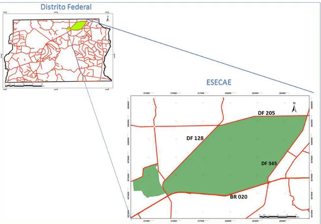
09 km). These road sections delimit a protected area, named Águas Emendadas-ESECAE Ecological Station (10,000 ha), which is recognised by UNESCO as a core area of the Cerrado Biosphere Reserve (Figure 02).
Figure 1. The large green area is the Águas Emendadas Ecological Station – ESECAE, in Brasília, Federal District of Brazil.
2.2.2. Data Collection
hotspot analyses were performed considering all the events without taxonomic or functional distinction.
2.2.3. Data analysis
We performed the hotspot analysis using both the Hotspot 2D formula and Malo’s method, with a 200 m radius. For the application of the new method, the result obtained for the radius of 200 m was weighted in windows of 2,800 m. For all methods, the null models were formed by 1000 random Poisson distributions.
To analyse the influence of the heterogeneity of the distribution on identified hotspots we remove each of the four highways that compose the study area from the analysis, one at a time, disregarding their extensions and number of events that occurred there.
The aggregation profile observed on the non-removed sections was compared with that obtained for the same stretches in the control analysis. That is, the analysis performed without removal of any road.
A confusion matrix was also used to compare the results before and after the removal of each highway using the ‘appearance’ – False Positive Classifications – or
‘disappearance’ – False Negative Classification – of hotspots, as well as by the geographical distribution of classification divergences.
3. RESULTS
3.1 Simulated study
We performed 420 hotspot analyses for each of the sample units combinations of ‘r’ and ‘w’ for the Windowned method, and ‘r’ for the Hotspot 2D and Malo’s methods,
considering the combination of noise types and density, with 21 simulations conducted for each.
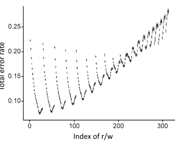
According to figure 3, the lowest error rates occurred for smaller radii. However, when considering each radius separately, the error rates decrease as the observation window radius increases until reaching a certain radius for which the larger the ‘w’
Figure 3. Results obtained from each division of radii ‘r’ and windows ‘w’
considering the 20 scenarios of noise type and density. These graphics were formed by different series of queued points. Each sequence of points represents a radius ‘r’, and each point, present in each row, represents the average obtained by bootstrap for each combination of this radius with a window ‘w’, totalling 3.
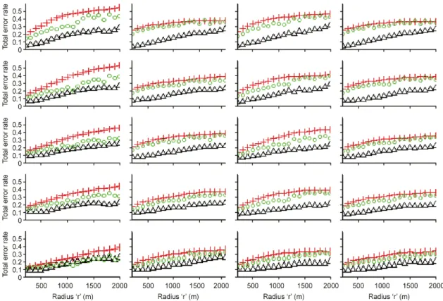
The results obtained for each combination of noise type and density is illustrated in Figure 4. For this analysis and the others in sequence, only the best result obtained for each radius for the new method was selected. The error rates from the new methodology are smaller than those from Hotspot 2D and Malo’s method. However, these values tend to be closer with decreasing density (graphs on the bottom line of the figure 4).
Index of r/w
Tot
al
err
or r
at
Figure 4 In this figure, each chart column represents one of the four types of noise illustrated in figure 1 B-E, following the same sequence from the first to the fourth column. The lines represent densities, with the density decreasing in the downward direction. The red crosses represent the total error rate values obtained with the Hotspot 2D formula for each radius, the green circles are the results of Malo’s method, and the black triangles are values achieved with the new methodology.
For Hotspot 2D and Malo’s methodologies, the results reveal a slight inversely
new method and the other two methodologies. For the Hotspot 2D and Malo’s methods, shorter densities present greater accuracy, whereas for the new method, the higher the density of events, the lower the error rate was. At least, considering only the best analysis scales for all type of noise, the Total error rate for Windowned Method was smaller than the others (Figure 5-D). Besides that, despite the type of noise, the new method results were significantly the same, while the accuracies of the Hotspot 2D and Malo’s methods vary according to the type of noise (Figure 5-D).
3.1 Real data study
During the five years of collection, we recorded the carcasses of 1,251 birds, 370 reptiles, 282 mammals and 150 amphibians, totaling 2,053 records. Of these records, we found 53% on the BR-020, 35% on the 128, 10% on the 345 and 2% on the DF-205.
The total length of the sections indicated as hotspots (black stretches in figure 6) for Malo’s method – 7.6 km – was much smaller than that indicated by the other two
methods, both of which identified 16.9 km as hotspots (Figure 6). However, the new methodology presented 30 stretches with an average extension of 0.563 km ± 0.438 km, while Hotspot 2D indicated 11 hotspots with a mean extension of 1.537 km ± 1.891 km, and Malo identified 14 stretches with an average length of 0.542 km ± 0.946 km.
The hotspots proposed by the Hotspot 2D and Malo’s methods are concentrated in two highways (BR-020 and DF-128), and both indicate a large continuous stretch as a hotspot on BR-020, with 6.7 km for Hotspot 2D and 3.8 km for Malo. Meanwhile, the new methodology indicates significant aggregations in all the highways, and the biggest continuous stretch is 1.8 km in length.
According to figure 5 B, almost all of the BR-020 highway is considered to be a hotspot. However, refining the methodology with window weighting, it is possible to verify that, within this large region susceptible to mitigation, there are areas whose density is significantly higher than the already high density of the stretch. Thus, justifying the identification of these points for proposed mitigation measures.
In the experiment with highway removal, all methods show variation in the correct classification of a stretch as a hotspot (table 2). For the Malo and Hotspot 2D methods the false positives only occurred when the BR-020 and DF-128 roads were removed, and the opposite occurred for the DF-205 and 345 highways.
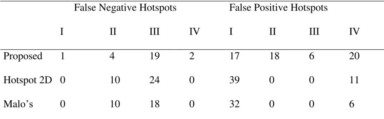
Table 1. Number of hotspots that ‘appeared’ - False Positive Hotspot -and ‘disappeared’ - False Negative Hotspot - due to the withdrawal of a highway in the analysis of hotspots.
False Negative Hotspots False Positive Hotspots
I II III IV I II III IV
Proposed 1 4 19 2 17 18 6 20
Hotspot 2D 0 10 24 0 39 0 0 11
Malo’s 0 10 18 0 32 0 0 6
I-Dataset analyzed without BR-020; II - Dataset analyzed without DF-345; III - Dataset
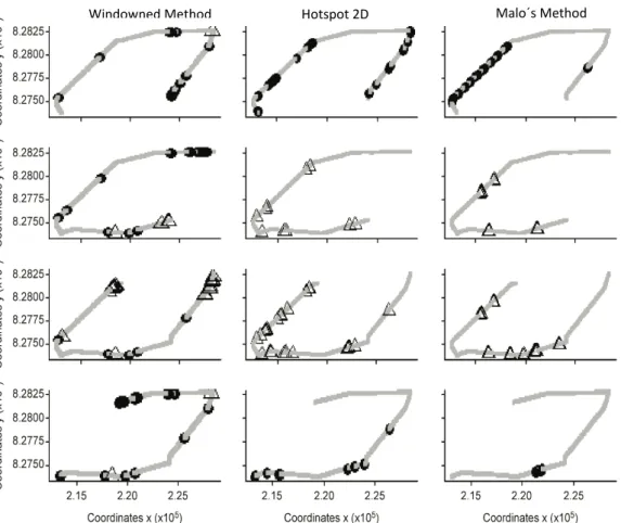
However, for the Windowned method, most of the classification errors occurred near the edges of the road stretches contiguous to the removed highway. For the other methods, the number of errors was much higher when BR-020 was removed, and the classification error pattern became more marked. The removal of BR-020 and DF-128 resulted in the appearance of false hotspots, while the removal of DF-205 and DF-345 resulted in the disappearance of true hotspots (Figure 6).
Figure 4. The columns represent the results obtained using the Windowned method, Hotspot 2D and Malo’s method, respectively. Each of the lines represents the removal of a highway from the study area, and in the downward direction, we have the removal of BR-020, followed by DF-345, DF-205 and finally DF-128. The triangles represent original hotspots that were not classified as such by the analysis with the
removal of a highway, and the circles are the points not originally identified as hotspotsbut have been classified as such in the analyses
4. DISCUSSION
Our results from the simulated study indicate that regardless of the method used and the scenarios of the event distributions the Windowned methodology application is less sensitive to the point pattern distribution first-order heterogeneity than the other methods analyzed (figure 3). Moreover, the smaller the analysis radius, the lower the sensitivity of the method was to the influence of the first-order effects of the distribution of point events on the identification of second-order processes. This situation goes against the common use of Ripley’s K function as a tool to identify radii for which the
aggregation is nonrandom. In this study, the study radius for hotspot definition can be determined (Mountrakis & Gunson 2009, Danks & Porter 2010, Coelho et al. 2012, Langen et al. 2012, Teixeira et al. 2013).
It is important to note that Ripley’s K statistic has been subject to many questions (e.g., Wiegand & A. Moloney 2004, 2014, Schiffers et al. 2008, Marcon & Puech 2009), mainly related to the so-called virtual aggregation effect. Thus, the use of Ripley’s K statistic may lead to choices that reflect virtual aggregation in hotspot
analysis.
Other relevant information that can be obtained from the simulated study is the effect of density on method accuracy. It is expected that increased sampling effort results in greater method efficiency. The results obtained with the Windowned method support this assertion. However, the accuracies of the Hotspot 2D and Malo’s methods
noise types is also important to note. Regardless of the kind of noise tested, the Windowned method experienced little variation in the accuracy of its results. The fact that Malo’s and Hotspot 2D methods presented oscillations in accuracy with changes in
the distribution profile shows that those methodologies are more sensitive to first-order heterogeneities. As each highway has a different profile, it is not possible to determine which type of highway the formulas will be more or less efficient.
The real data study presents a large difference in the classifications generated by the different methodologies. The Hotspot 2D formula generated a hotspot pattern that reflects more the effects of the landscape on roadkills than punctual processes. The vast stretches of hotspots generate uncertainty about the ideal locations for implementing mitigation measures. Malo’s method is more accurate than Hotspot 2D, indicating small
stretches as hotspots, but both identify significant aggregations only on the roads that present greater regional intensities in event occurrences.
Unlike the other methods, the method proposed in this article indicated significant points of aggregation along the four highways, making it possible to verify points with a higher probability of being hit on highways with low densities of events. Also, the map presents another significant finding: according to figure 5 B, almost all of the BR-020 highway is considered to be a hotspot. However, when refining the methodology with window weighting, it is possible to check that, within this broad region susceptible to mitigation, there are areas where density is significantly higher than the previous high density of the stretch, justifying the identification of these points for proposed mitigation measures.
table 2) increases the number of hotspot classifications. The increase occurs because the null model takes into account the ratio between the number of individuals and road length, removing a considerable number of events. The lambda value tends to decrease, reducing the threshold value for classification as a hotspot, even though there is no variation in the records of this section. This effect is also observed when the removal of a small-density highway causes the threshold value to increase, causing some points to cease to be significant aggregations, even though there has been no change in the number of records at those points.
Notwithstanding these peculiarities, the three methodologies presented changes in the classification of stretches as hotspots. The explanation for these changes in all cases is the null model used. When applying a Poisson distribution for all highways, even with notorious variations in roadkill density, a road with a high density of events determines the classification of the other roads, even in some cases when there is independence between the registers. Borda-de-Agua et al. (2016) questioned the use of the Poisson distribution as a null model owing to the high probability of type II errors.
much lower than that at other non-identified points. This fact does not mean that mitigation priority should be given to points with fewer records, though these points may help to compose aggregation models based on the surrounding environmental characteristics.
Considering the four possibilities for dealing with the non-homogeneities in the point distribution of events proposed by Wiegand & Moloney (2014), state of the art in road ecology still using the alternative of ignoring this characteristic in analyses of roadkills aggregation. This paper begins the debate on the application of other alternatives, proposing a methodological change to avoid or reduce the effects of heterogeneity by using observation windows.
Although this article goes beyond the first option, this approach should be better by using a more rigorous method for delineating homogeneous sub areas. Our results minimized part of the heterogeneity effect in the pattern, but the windows used still reflect a weak signal of heterogeneity. The subdivision of a studied highway into minimally homogeneous segments can be carried out in several ways. Using one or more landscape and traffic characteristics that show a significant correlation with the trampling of the species of interest. Using cluster identification techniques, such as a method based on the similarity between neighbors called Shared Nearest Neighbour (SNN), created by Jarvis & Patrick (1973) and improved upon by Ertöz, Steinbach& Kumar(2003). The algorithm of this method finds the nearest neighbors of each data point and then redefines the similarity between pairs of points regarding how many nearest neighbors the two points share.
proposition of null models with heterogeneous Poisson distributions, or changes in the metrics used in road ecology, as proposed in Ang, Baddeley & Nair (2012).
5. CONCLUSION
This paper introduces the debate on the application of other alternatives, proposing a methodological change to avoid or diminish the effects of heterogeneity by using observation windows. The Windowned method can be used as a way to minimize the effect of the first-order heterogeneity of a distribution of point events on or along a linear network. The main utility of this method is its ability to identify smaller stretches with intensities greater than expected in the interior of a zone with a high intensity of roadkill, which improves the process of choosing sites for mitigation.
The method should not be applied in a unique way for the proposal of mitigation measures, since the identification of hotspots in areas with low roadkill density may not always indicate a mitigable intensity. However, the identification of these points, which do not usually appear in traditional hotspot analyses, can improve the proposition of landscape-based models.
6. ACKNOWLEDGEMENTS
7 BIBLIOGRAPHY
Ang, Q. W., Baddeley, A., &Nair, G. (2012). Geometrically corrected second order analysis of events on a Linear Network, with applications to ecology and criminology. Scandinavian Journal of Statistics, 39, 591–617. doi:10.1111/j.1467-9469.2011.00752.x.
Baddeley, A. J., Møller, J., &Waagepetersen, R. (2000). Non- and semi-parametric estimation of interaction in inhomogeneous point patterns. Statistica Neerlandica, 54, 329–350. doi:10.1111/1467-9574.00144.
Baddeley, A., Rubak, E., &Turner, R. (2015). Spatial Point Patterns: Methodology and Applications with R. CRC Press, Boca Raton, FL.
Baddeley, A., &Turner, R. (2005). spatstat: An R Package for Analyzing Spatial Point Patterns. Journal of Statistical Software, 12. doi:10.18637/jss.v012.i06.
Barrientos, R., &Plaza, M. (2016). Road-kill hot spots can change over the time, variables explaining them do not. International Conference on Ecology and Transportation, Programme and Abstracts. (ed. É.Guinard), p. 288. CEREMA,
Lyon, France.
Beaudry, F., DeMaynadier, P. G., &Hunter, M. L. (2008). Identifying road mortality threat at multiple spatial scales for semi-aquatic turtles. Biological Conservation, 141, 2550–2563. doi:10.1016/j.biocon.2008.07.016.
Ecology and Transportation, Programme and Abstracts (ed É. Guinard), p. 286.
CEREMA, Lyon, France.
Coelho, A. V. P., Coelho, I. P., Teixeira, F. Z., &Kindel, A. (2014). Siriema: Road Mortality Software. User´s Guide. NERF/UFRGS, Porto Alegre, Brasil.
Coelho, I. P., Teixeira, F. Z., Colombo, P., Coelho, A. V. P., &Kindel, A. (2012). Anuran road-kills neighboring a peri-urban reserve in the Atlantic Forest, Brazil.
Journal of Environmental Management, 112, 17–26.
doi:10.1016/j.jenvman.2012.07.004.
Costa, A. S., Ascensão, F., &Bager, A. (2015). Mixed sampling protocols improve the cost-effectiveness of roadkill surveys. Biodiversity and Conservation, 24, 2953– 2965. doi:10.1007/s10531-015-0988-3.
Danks, Z. D., &Porter, W. F. (2010). Temporal, spatial, and landscape habitat characteristics of moose–vehicle collisions in western Maine. Journal of Wildlife Management, 74, 1229–1241. doi:10.2193/2008-358.
Eberhardt, E., Mitchell, S., &Fahrig, L. (2013). Road kill hotspots do not effectively indicate mitigation locations when past road kill has depressed populations. Journal of Wildlife Management, 77, 1353–1359. doi:10.1002/jwmg.592.
Grilo, C., Bissonette, J. A., &Santos-Reis, M. (2009). Spatial–temporal patterns in Mediterranean carnivore road casualties: Consequences for mitigation. Biological Conservation, 142, 301–313. doi:10.1016/j.biocon.2008.10.026.
Jarvis, R. A., &Patrick, E. A. (1973). Clustering using a similarity measure based on shared near neighbors. IEEE Transactions on Computers, C–22, 1025–1034. doi:10.1109/T-C.1973.223640.
Langen, T. A., Gunson, K. E., Scheiner, C. A., &Boulerice, J. T. (2012). Road mortality in freshwater turtles: Identifying causes of spatial patterns to optimize road planning and mitigation. Biodiversity and Conservation, 21, 3017–3034. doi:10.1007/s10531-012-0352-9.
Liu, Q., Li, Z., Deng, M., Tang, J., &Mei, X. (2015). Modeling the effect of scale on clustering of spatial points. Computers, Environment and Urban Systems, 52, 81–92. doi:10.1016/j.compenvurbsys.2015.03.006.
Malo, J. E., Suárez, F., &Díez, A. (2004). Can we mitigate animal-vehicle accidents using predictive models?Journal of Applied Ecology, 41, 701–710. doi:10.1111/j.0021-8901.2004.00929.x.
Marcon, E., &Puech, F. (2009). Generalizing Ripley ‘s K function to inhomogeneous
populations. HAL archives-ouvertes.fr, HAL Id: halshs-00372631.
Mountrakis, G., &Gunson, K. (2009). Multi-scale spatiotemporal analyses of moose– vehicle collisions: A case study in northern Vermont. International Journal of
Geographical Information Science, 23, 1389–1412.
doi:10.1080/13658810802406132.
Nychka, D., Furrer, R., Paige, J., &Sain, S. (2015). Fields: Tools for Spatial Data. doi:10.5065/D6W957CT.
R Core Team. (2016). R: A language and environment for statistical computing. R Foundation for Statistical Computing. Retrieved from http://www.R-project.org.
Ramp, D., Caldwell, J., Edwards, K. A., Warton, D., &Croft, D. B. (2005). Modelling of wildlife fatality hotspots along the Snowy Mountain Highway in New South Wales, Australia. Biological Conservation, 126, 474–490. doi:10.1016/j.biocon.2005.07.001.
Santos, R. A., Santos, S. M., Santos-Reis, M., Picanço de Figueiredo, A., Bager, A., Aguiar, L. M., &Ascensão, F. (2016). Carcass persistence and detectability : Reducing the uncertainty surrounding wildlife-vehicle collision surveys. PLOS One, 11, e0165608. doi:10.1371/journal.pone.0165608.
Santos, R. A., Ascensão, F., Ribeiro, M. L., Bager, A., Santos-Reis, M., &Aguiar, L. M. S. (2017). Assessing the consistency of hotspot and hot- moment patterns of wildlife road mortality over time. Perspectives in Ecology and Conservation, 15, 56–60. doi:10.1016/j.pecon.2017.03.003.
Implications for survey design. Journal of Environmental Management, 162, 87–95. doi:10.1016/j.jenvman.2015.07.037.
Schiffers, K., Schurr, F. M., Tielbörger, K., Urbach, C., Moloney, K., &Jeltsch, F. (2008). Dealing with virtual aggregation - A new index for analysing heterogeneous point patterns. Ecography, 31, 545–555. doi:10.1111/j.0906-7590.2008.05374.x.
Seiler, A., Sjölund, M., Andrasik, R., Rosell, C., Torrellas, M., Sedonik, J., Bíl, M., &Jägerbrand, A. (2016). Are animal-vehicle collisions a random event? – Analysis of the spatial distribution of accident data. International Conference on Ecology and Transportation, Programme and Abstracts. (ed. É.Guinard), p. 290.
CEREMA.
Seo, C., Thorne, J. H., Choi, T., Kwon, H., &Park, C.-H. (2015). Disentangling roadkill: The influence of landscape and season on cumulative vertebrate mortality in South Korea. Landscape and Ecological Engineering, 11, 87–99. doi:10.1007/s11355-013-0239-2.
Teixeira, F. Z., Coelho, I. P., Esperandio, I. B., Oliveira, N. R., Peter, F. P., Dornelles, S. S., Delazeri, N. R., Tavares, M., Martins, M. B., &Kindel, A. (2013). Are road-kill hotspots coincident among different vertebrate groups?Oecologia Australis, 17, 36–47. doi:10.4257/oeco.2013.1701.04.
VanDerWal, J., Falconi, L., Januchowski, S., Shoo, L., &Storlie, C. (2014). SDMTools: Species Distribution Modelling Tools: Tools for Processing Data Associated
with Species Distribution Modelling Exercises. – R package ver. 1.1-20, <
http://CRAN.R-project.org/package = SDMTools >.
Wiegand, T., &Moloney, K. A. (2004). Rings, circles, and null-models for point pattern analysis in ecology. Oikos, 104, 209–229. doi:10.1111/j.0030-1299.2004.12497.x.
CAPÍTULO 02 – DEFINIÇÃO DA CURVA DE PRECISÃO PARA ANÁLISE DA SUFICIÊNCIA AMOSTRAL EM ECOLOGIA DE ESTRADAS
RESUMO
Em uma pesquisa científica, a amostra deve ter o tamanho suficiente para validar os resultados sem representar, no entanto, um desperdício de recurso e tempo. Para este capítulo testou-se a hipótese de que a precisão da análise de agregação de atropelamentos de fauna com o tamanho da amostra pode ser utilizada para estabelecer a suficiência amostral. Os valores de precisão de classificação de hotspot foram obtidos comparando-se vinte e um conjuntos de dados simulados, a partir de reamostragens com reposição de registros reais de atropelamentos, com cada um de seus subconjuntos, resultados de divisões de três a dez vezes do conjunto da amostra simulada. Utilizou-se regressão quantílica entre os valores de precisão e o logaritmo dos tamanhos dos subconjuntos dos quais as precisões foram obtidas. Nesta regressão foram simulados os quantis 2,5%, 50% e 97,5% para representar três cenários de grau de eficiência do método de classificação de hotspots, do menos ao mais eficiente. Os resultados demonstraram que existe correlação positiva entre a precisão de classificação de hotspots com o tamanho da amostra e que esta relação é válida para diferentes formas
Este método dá robustez às proposições de medidas mitigadoras, uma vez que garante o grau de precisão dos locais indicados.
Palavras-chave: coleta de dados, licenciamento ambiental, medidas mitigadoras, regressão quantílica, rodovias, suficiência amostral.
ABSTRACT
to mitigating measures propositions, since it guarantees the precision degree of the indicated places.
INTRODUÇÃO
A definição do tamanho amostral é uma decisão muito importante em qualquer planejamento para uma pesquisa científica, pois amostras muito grandes representam desperdício de recursos, enquanto que muito pequenas diminuem a aplicabilidade e robustez dos resultados (Cochran 1977).
Dois vieses reduzem a eficiência das coletas de dados em Ecologia de Estradas: o tempo de permanência das carcaças nas rodovias e a capacidade de detecção destas carcaças pelo pesquisador (Slater 2002, Santos et al. 2011, 2016, Teixeira et al. 2013, Collinson et al. 2014). Estes fatores interferem no tempo de duração necessária do experimento para se atingir um tamanho amostral suficiente para as análises pretendidas. Para diminuir o efeito do tempo de permanência das carcaças nas rodovias, é recomendado curto períodos de tempo entre as campanhas, no máximo uma semana, se o objetivo do estudo é a identificação da riqueza de espécies afetadas (Bager & da Rosa 2011). No entanto, para a redução da probabilidade de falsa indicação de hotspots de atropelamento recomendam-se coletas diárias ou com um dia de intervalo (Santos et al. 2015).
A correção do viés de detecção pode se dar pela redução da velocidade de deslocamento durante a busca pelas carcaças. Alguns estudos são realizados à pé (Attademo et al. 2011, Coelho et al. 2012, Skórka et al. 2015) ou de bicicleta (Garriga et al. 2012, Eberhardt et al. 2013, Garrah et al. 2015). Porém, em função da necessidade
de se realizar grandes deslocamentos para os registros dos atropelamentos, a grande maioria dos estudos é realizada em automóveis.
intervalo, e com deslocamentos com velocidade não superior a 20km/h (Collinson et al. 2014). No entanto, as formas de registro, frequência de coletas de dados e duração das amostragens têm grande variação entre os pesquisadores. Encontra-se na literatura estudos com coletas não sistemáticas (Mountrakis & Gunson 2009) ou coletas sistemáticas que variaram entre 80 dias consecutivos de bicicleta (Eberhardt et al. 2013), três anos de monitoramento semanal a pé (Skórka et al. 2015) ou mesmo em cinco anos de monitoramento com carro, realizadas parte diariamente e parte a cada dois dias (Seo et al. 2013).
Normalmente os protocolos de pesquisa são definidos com base nos custos envolvidos e na capacidade operacional (Cochran, 1977). Nos casos em que o protocolo ideal é inviável, o pesquisador pode optar por duas decisões: ou se abandona os esforços até conseguir mais recursos, ou assume-se a redução do tamanho amostral, reduzindo a precisão das análises (Cochran, 1977). Neste sentido, conhecer a relação entre o tamanho da amostra e a precisão dos resultados que ela oferece é uma das importantes informações a se obter para decidir pelo término do esforço de coleta de dados.