Vision, Image Signal Processing

Which Differintegration? 1

Manuel D. Ortigueira1, J. A. Tenreiro Machado2, J. Sá da Costa3

1 _{UNINOVA and Faculdade de Ciências e Tecnologia da Universidade Nova de Lisboa}

Campus da FCT da UNL, Quinta da Torre

2825 - 114 Monte da Caparica, Portugal

mdo@uninova.pt

2

Dept. of Electrotechnical Engineering

Instituto Superior de Engenharia do Porto

Rua Dr. Antonio Bernardino de Almeida

4200-072 Porto, Portugal

jtm@dee.isep.ipp.pt

3 _{Dept. of Mechanical Engineering}

Instituto Superior Técnico

Universidade Técnica de Lisboa

Av. Rovisco Pais 1, 1049-001 Lisbon, Portugal

sadacosta@dem.ist.utl.pt

Abstract:

Despite the great advances in the theory and applications of fractional calculus, some topics remain

unclear making a systematic use difficult. In this paper the fractional differintegration definition

problem is studied from a systems point of view. Both local (Grünwald-Letnikov) and global

(convolutional) definitions are considered. It is shown that the Cauchy formulation should be adopted

since it is coherent with usual practice in signal processing and control applications.

1. INTRODUCTION

Fractional calculus is an area of mathematics that deals with derivatives and integrals of non

integer order (i.e., real or, even, complex) that are joined under the name of differintegration. In the

last decade, fractional calculus has been rediscovered by physicists and engineers and applied in an

increasing number of fields [1-3], namely in the areas of signal processing, control engineering and

electromagnetism [4-10, 18-20]. Despite the progress that has been made, several topics remain

without a clear and concise formulation. Surprisingly, one of them is the definition of Fractional

Differintegration (FD). In fact, there are several definitions that lead to different results [11-13],

making the establishment of a systematic theory of fractional linear systems difficult. In facing this

problem, we can adopt one of the following strategies:

• Choose a formulation, a priori, on the basis of a personal preference;

• Decide to work in a functional space where all the definitions give the same result [14]. However,

this strategy is interesting only when solving differential equations with inputs in the same

space;

• Choose formulations that assure a generalization of common and useful results or tools.

Bearing these ideas in mind, in this paper we will adopt the third point of view since it is the one

that allows building a systematic theory of fractional linear system that resembles the theory of linear

(integer order) systems.

The fact of dealing with non-integer order derivatives and integrals constitutes one of the major

advantages in using fractional calculus, because solutions are general functions rather than being

constrained to the exponential type. Consequently, we are interested in generalising the useful, and

well known results, but there are noteworthy differences in this generalization. Integer-order

derivatives depend only on the local behaviour of a function, while fractional derivatives depend on

the whole history of the function [15]. Therefore, the problem is not just a simple matter of

substituting the integer derivative by the fractional derivative; a proper definition of fractional

derivative is needed. Moreover, it is important that the adopted definition preserves both the properties

of the integer-order differintegration calculus and the fundamental concepts and proprieties of system

As said previously there are several distinct definitions of FD that are equivalent for a wide class of

functions [1,13]. Nevertheless, from an engineering point of view most formulations reveal

compatibility problems with the usual signal processing and systems theory practice. In fact, in signal processing, we often assume that signals have ℜ as domain and use the Bilateral Laplace and Fourier Transforms as key tools. Based on these tools, the important concepts of transfer function and

frequency response are defined, with properties that we want to preserve in the fractional case. In this

line of thought, different differintegration definitions from a common framework are considered in this

article and compared in order to establish a practical mathematical tool. Without loosing generality,

we consider two possibilities for the definition of FD in this work:

• An approach based on the generalisation of the usual derivative definition, that is, the Grunwald-Letnikov derivative and integral definitions,

• A global approach based on a convolutional formulation.

As known, any function can be defined in a space isomorphic to a space in which it has been

defined in. Thus, it is possible to define the FD through its properties in certain transformed space

corresponding to some common transforms like the Laplace Transform (LT). Our starting point is the

generalization of the well known property of the LT, corresponding to the time domain differentiation:

LT[DP

α

P

f(t)] = sP

α

PF(s), α ∈ ℜ (1)

where D denotes the derivative, f(t) is a signal with (two-sided) Laplace Transform F(s) (T

2

T

). If α > 0 we have a fractional derivative; if α < 0 it is a fractional integral. With this formulation the

fractional integral and derivative are mutually inverse operations, which bring an important

consequence: the fractional derivative and integral are inverse operations that commute (semigroup

property):

DP

α

P

{DP

β

P

} = DP

α+β

P

= DP

β

P

{DP

α

P

}, α, β ∈ ℜ (2)

Unfortunately, this property is not valid in most differintegration definitions [1, 13], as it is the so

called Miller-Ross sequential derivative [1] and all the definitions that use a proper sub-set of ℜ.

From a system point of view, we are looking for a “differintegrator” such that its transfer function

is given by sP

α

P

, provided that we have fixed a suitable branch cut line, since it is a multi-valued

expression. There are infinite possibilities, but proceeding as Zavada [16], we choose the negative

half-axis. It is clear that if we choose this branch cut line then we force the region of convergence of

the LT to be the right (Re(s)> 0) or the left (Re(s)< 0) half plane. This has an important consequence,

T

2

T

namely that Uthe differintegrator must be either causal or anti-causalU, as in the usual negative integer

case, contrarily to the common integer derivatives that are neither causal nor anti-causal (acausal).

In this line of thought, this paper is organized as follows. In sections two and three we discuss two

distinct perspectives to differintegration, namely the Grünwald-Letnikov and the convolution

approaches, respectively. Based on the previous results, section four shows an example common in

signal processing and systems theory practice. Finally, section five draws the main conclusions.

2. GRÜNWALD-LETNIKOV DIFFERINTEGRATION

2.1. Derivatives

Grünwald-Letnikov derivatives are generalisations of the usual derivative definitions. Therefore, sP

α

P

(α > 0) can be considered as the limit when h ∈ ℜP

+

P

tends to zero in the right hand sides of the

following expressions:

sP

α

P

= T lim h→0+

(1 − e-sh)α

hα T (3a)

sP

α

P

= T lim h→0+

(esh − 1)α

hα T (3b)

On the other hand, we can use the binomial series to obtain:

TA

(1 − e-sh)α

hα =

1

hα

∑

∞

(−1)k

_⎝

⎛

_⎠

⎞

k e

−sh

E

k

EA

, TRe(s) > 0 (4a)

TA

(esh − 1)α hα =

(−1)α

hα

∑

k = 0 ∞

(−1)k

_⎝

⎛

_⎠

⎞

k e

sh

E

k

EA

, TRe(s) < 0 (4b)

In the integer order cases, the right sides in the above expressions are identical. With these

formulae, we can write:

sP

α

P

= TA lim h→0+ 1 hP α P

∑

∞

(−1)k

_⎝

⎛

_⎠

⎞

k e

−sh

E

k

EA

, TRe(s) > 0 (5a)

sP

α

P

= A lim

T

h→0+

(−1T)

α

hα

∑

∞

(−1)k

_⎝

⎛

_⎠

⎞

k e

sh

E

k

EA

Note the right hand sides regions of convergence. This means that (5a) and (5b) lead to causal and

anti-causal derivatives, respectively. When inverted to the time domain, these expressions correspond,

respectively, to (T

3

T

):

A

DαT

+(t) = lim_h→0+ 1

hα

∑

∞

(−1)k

_⎝

⎛

_⎠

⎞

k δ(t − khE)EA (6a)

TA

Dα₋(t) = lim

h→0+

(−1)α

hα

∑

k = 0 ∞

(−1)k

_⎝

⎛

_⎠

⎞

k δ(t + kh)EEA (6b)

where δ(t) is the Dirac delta impulse.

Let f(t) be a limited function and α > 0. The convolution of (6a) and (6b) with f(t) leads to the

Grünwald-Letnikov forward and backward derivatives:

f(α)

+ (t) = A lim h→0+

∑

∞

(−1)k

_⎝

⎛

_⎠

⎞

k f(t − kh)

hαE

EA

(7a)

f(α)₋ (t) = A lim h→0+ (−1)

αk = 0

∑

(−1)k

_⎝

⎛

_⎠

⎞

k f(t + kh)

hαE

EA

(7b)

Both expressions agree with the usual derivative definition when α is a positive integer. Moreover,

expression (7a) corresponds to the left-hand sided Grünwald-Letnikov fractional derivative while (7b) has the extra factor (−1)P

α

P

, when compared with the right-hand sided Grünwald-Letnikov fractional

derivative [13]. Therefore, (7a) and (7b) should be adopted for right and left signals (T

4

T

), respectively.

In [13] the convergence properties of the above series are studied. It is noteworthy that we can have

the forward derivative without the backward one existing and vice-versa. For example, let us apply

both definitions to the function f(t) = eP

at

P

. If a > 0, expression (7a) converges to f(α)

+ (t) = aP

α

PeP

st

P

, while

(7b) diverges. On the other hand, if f(t) = eP

−at

P

equation (7a) diverges while (7b) converges to f(α)₋ (t) =

(−a)P

α

PeP

−at

P

.

Within these definitions, we can apply (7a) or (7b) successively for different values of α, leading

also to a multi-step derivative DP

α

P

= DP

β

PDP

γ

PDP

µ

P

… DP

λ

P

, with α = β + γ + µ + … + λ. This means that we

T

3

T

We do not address the problem of the convergence of the series here {see [17]}.

T

4

T

have infinite ways of performing a fractional derivative. However, the order in which the fractional

differential operators are concatenated is relevant. This is a very important matter that has originated a

lot of problems mainly when solving fractional differential equations under non zero initial conditions

[9]. When α is negative the series is divergent, in general, and an alternative definition needs to be

derived as shown in the next section.

2.2. Integrals

The expressions for the Grünwald-Letnikov derivatives are not useful for integration [13]. We

should expect this because _{1 −} h

e−sh ≈

1

s is a poor approximation and, in fact the bilinear expression

h

2

1 + e−sh

1 − e−sh ≈

1

s is superior. Therefore, we can adopt the second approximation to define the fractional

integration, leading to a more suitable form for the fractional integral computation.

For small h ∈ ℜP

+

P

:

A

1

sα ≈

⎝

⎛

⎠

⎞

h

2

1 + e-sh

1 − e−sh

α = h

α

2α

∑

n = 0 ∞ Cα n e −sh E n EA

, Re(s) > 0 (T

5

T

) (8)

where

Cα

n =

∑

n (−1)k

⎝

⎛

⎠

⎞

⎝

⎛

⎠

⎞

n−k n ≥ 0 (9)

is the convolution of the coefficients of two binomial series. We can give another form to (9). As

⎝

⎛

⎠

⎞

k = (−1)

k(−a)k

k! (10)

where (a)Bn B= a(a+1)…(a+n−1) is the Pochhammer symbol and remarking that n! = (−1)P

k

P

(−n)BkB(n−k)!

and (a)BnB = (−1)P

k

P

.(−a−n+1)BkB(a)Bn−kBfor k ≤ n, we obtain:

Cα

n = (−1)

n(−α)n

n!

∑

k = 0

n _(α)

k(−n)k

(−α − n + 1)k

(−1)k

k! (11)

or

Cα

n = (−1)

n(−α)n

n! 2F1[(α,−n, −α − n + 1,−1] (12)

T

5

T

where B2BFB1B is the Gauss Hypergeometric function [2]. Consequently, approximation (8) leads to a

Grünwald-Letnikov like fractional integral of order α for a function f(t):

fP

(α)

P

(t) = lim

h→0+ hα

2α

∑

n = 0 ∞

Cα

n f(t − nh), α < 0 (13)

For causal signals and h > 0, the series in (7a) and (13) become finite summations. The formulation

(12) is interesting because it allows us to compute Cα

n recursively. In fact, although the Gauss

hypergeometric function does not have a closed form for those arguments it satisfies the following

recursion [6]:

f(n) = _α+2α

n−1f(n−1) +

(n−1)(n−2)

(α+n−1)(α+n−2)f(n−2) (14)

with f(0) = 1, and f(1) = 2.

3. CONVOLUTIONAL DIFFERINTEGRATION

Here we address the linear system case (the Differintegrator) that has sP

α

P

- with Re(s)>0 or

Re(s)<0) – as Transfer Function. To find its Impulse Response, we look for the inverse Laplace

transform of sP

α

P

, δP

(α)

P

(t), with α ∈ ℜ. So the differintegration of a signal f(t) is given by the convolution

of f(t) with δP

(α)

P

(t). To present this convolutional differintegration definition, we introduce the following

distributions:

δ(−ν)_± (t) = ± t

ν−1

Γ(ν)u(±t), 0 < ν < 1 (15)

and

δ(_±n)(t) =

⎩

⎨

⎧

δ(n)_{(t) for n ≥ 0}

(16)

where n ∈ Z, δP

(α)

P

(t) is the α differintegrator of δ(t) and u(t) is the Heaviside unit step.

The differintegrations usually used [2] can be classified as right and left sided, respectively:

f(α)

r (t) = [f(t) u(t − a)] * δ

(n) + (t) * δ

(−ν)

+ (t) (17a)

f(α)

l (t) = [f(t) u(b − t)] * δ

(n) + (−t) * δ

(−ν)

The orders are given by α = n − ν, n being the least integer greater than α and 0 < ν < 1. In

particular, if α is integer then ν = 0 (T

6

T

). We must remark that, from our point of view, Uonly the cases a

= −∞ and b = +∞ cases are acceptableU. Otherwise, we are incorporating signal characteristics into a

definition that we think is wrong. We must state a definition valid for all functions. In other words, the

definition must be the same independently of the signal being differintegrated. With this in mind, we

rewrite (17a) and (17b) as:

f(α)

r (t) = f(t) * δ

(n) + (t) * δ

(−ν)

+ (t) (18a)

f_l(α)(t) = f(t) * δ₊(n)(−t) * δ(−ν)₊ (−t) (18b)

The LT of (18a) and (18b) are sP

α

P

X(s) and (−s)P

α

P

X(s), respectively, that differ on the factor (−1)P

α

P

.

This means that Uit is not a backward differintegration and therefore it is unsuitableU. From these

considerations, we are led to the expressions for the forward and backward differintegrations with

general format given by:

f(α)

+ (t) = f(t) * δ (n) + (t) * δ

(−ν)

+ (t) (19a)

f₋(α)(t) = f(t) * δ₋(n)(t) * δ(−ν)₋ (t) (19b)

With these formulae, integration and derivation are inverse operations. From different orders of

commutability and associability in the double convolution we can obtain distinct formulations. For

example, in the forward case we have respectively the Riemann-Liouville, the Caputo and the

Generalised functions (Cauchy) differintegration [2]:

f(β)

+ (t) = δ (n) + (t) * ⎩⎨

⎧

⎭ ⎬ ⎫

f(t) * δ(−ν)

+ (t) (20a)

f(β)

+ (t) = ⎩⎨ ⎧

⎭ ⎬ ⎫

f(t) * δ(₊n)(t) * δ(−ν)

+ (t) (20b)

f(β)

+ (t) = f(t) * ⎩⎨ ⎧

⎭ ⎬ ⎫ δ(₊n)(t) * δ(−ν)

+ (t) , n ∈ Z, 0 ≤ ν < 1 (20c)

We must remark that (20a) corresponds to a ν order integration followed by an n integer order

derivative, while in (20b) we have the reverse situation. Concerning equation (20c), the convolution

inside brackets is a generalised function given by [2,18,21]:

δ(β) + (t) =⎩⎨

⎧

⎭ ⎬ ⎫ δ(₊n)(t) * δ(−ν)

+ (t) =

t-β−1

Γ(−β)u(t), β=n−ν (21)

T

6

T

All the above formulae remain valid in the case of integer integration, provided that we put δP

(0)

P

which can be considered as Uthe Impulse Response of the fractional differintegratorU. With it we can

perform the computation in one step. Moreover, this formulation is a generalization of the well-known

Cauchy integral [12,13]. It is not difficult to obtain the corresponding backward formulations.

4. SELECTING A DIFFERINTEGRATION From previous sections it seems clear that:

• the above three formulations are equivalent when looked from the LT point of view.

• contrary to the Grünwald-Letnikov differintegration and (20c), the computation is done in

two steps in (20a) and (20b).

We can combine all the differintegrations in the sense that we can decompose the order as β=βB1B+βB2B+βB3+…+βB BnB and use any method to compute the βBiB (i = 1, …, n) differintegration.

This can lead us to a complicated situation or to results that are far from the expected. Consider the

following problem. We want to check if x(t) is the solution of the differential equation xP

(3/2)

P

(t) + a

xP

(1/3)

P

(t) + b xP

(1/5)

P

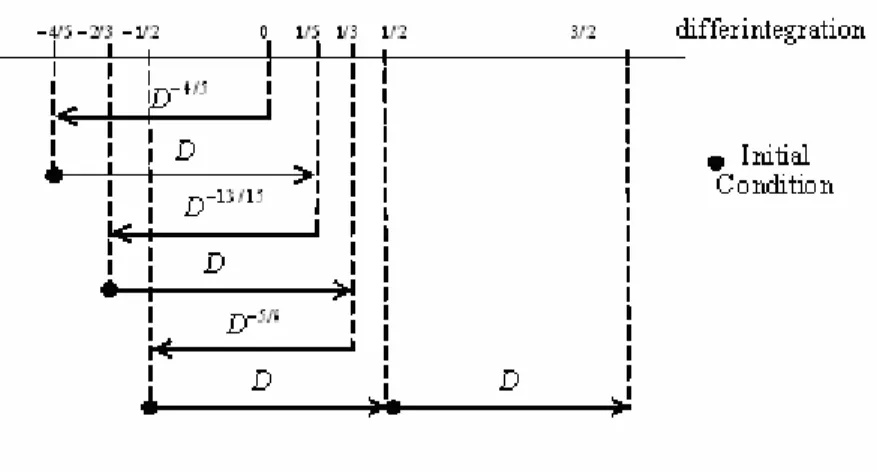
(t) = 0, a, b ∈ ℜ, for t > 0. We have the options:

a) In the Riemann-LiouvilleP Pformulation (20a), we have to compute 3 integrals and 4 integer

derivatives. In fact, if we want to compute the above derivatives sequentially we have to do

the following sequence of computations: xP

(1/5)

P

(t) = D[DP

−4/5

P

x(t)] → xP

(1/3)

P

(t) = D[DP

−13/15

P

xP

(1/5)

P

(t)]

→ xP

(3/2)

P

(t) = D{D[DP

−5/6

P

xP

(1/3)

P

(t)]}.

Figure 1 – steps and initial conditions in the Riemann-Liouville definition

b) In the Caputo formulation (20b) we have the same operations but the derivatives and

integrations are in reverse order: xP

(1/5)

P

(t) = DP

−4/5

P

[Dx(t)] → xP

(1/3)

P

(t) = DP

−13/15

P

[DxP

(1/5)

P

(t)] → xP

(3/2)

P

(t)

= DP

−5/6

P

{D[DxP

(1/3)

P

(t)]}.

Figure 2 – steps and initial conditions in the Caputo definition

c) In the Cauchy definition (20c) we have 3 fractional derivatives: xP

(1/5)

P

(t) = DP

1/5

P

x(t) → xP

(1/3)

P

(t) =

DP

2/15

P

[xP

(1/5)

P

(t)] → xP

(3/2)

P

(t) = DP

7/6

P

[xP

(1/3)

P

(t)].

On the other hand, we must remark that each time we perform an integer order derivative, we are

inserting initial conditions that may be meaningless in the problem at hand. In the sequence of

operations presented above, we introduce the following initial conditions [1,2,14]:

a) Riemann-Liouville case: DP

−4/5

P

x(t)|Bt=0+B, DP

−2/3

P

x(t)|Bt=0+B, DP

−1/2

P

x(t)|Bt=0+B, and DP

1/2

P

x(t)|Bt=0+B. To understand

these results, we only have to remember that D[f(t)u(t)] = D[fP

(α)

P

(t)].u(t) + fP

(α)

P

(0+).δ(t).

b) Caputo case: x(t)|Bt=0B, DP

1/5

P

x(t)|Bt=0B, DP

1/3

P

x(t)|Bt=0B, and DP

4/3

P

x(t)|Bt=0B. In this case, the fractional

integration does not insert an initial condition, contrarily to the integer order derivative. Then,

we have DP

−α

P

[f(t)u(t)]´ = DP

−α

P

[f´(t).u(t) + f(0+).δ(t)], leading to the result.

c) Cauchy case: x(t)|Bt=0B, DP

1/5

P

x(t)|Bt=0B, and DP

1/3

P

x(t)|Bt=0B. This result directly from the equation. Of

course, we can use other initial conditions by specifying other derivatives, even not “visible” in

the equation. For example, we can write: xP

(3/2)

P

(t) + 0.xP

(1)

P

(t) + 0.xP

(1/2)

P

(t) +axP

(1/3)

P

(t) + b xP

(1/5)

P

(t) = 0

and insert the corresponding initial conditions [14].

To exemplify, consider a simple circuit with two fractional capacitors [22]:

Figure 4 – Electrical circuit using fractional capacitors

The subscripts in C point the integration order, say. The impedance corresponding to a given

capacitor is given by _(jωCi)1 i with i = α or β [3]. We will assume that β ≥ α. It is not hard to show that

the input-output relation is given by:

aB3B.DP

α+β

P

vBoB(t) +aB2B.DP

β

P

vBoB(t) + aB1B.DP

α

P

vBoB(t) + vBoB(t) =vBiB(t)

and, also

aB3B.DP

α+β

P

vBaB(t) +aB2B.DP

β

P

vBaB(t) + aB1B.DP

α

P

vBaB(t) + vBaB(t) = bDP

β

P

vBiB(t) + vBiB(t)

with: aB1B = RCBαB, a2BB = 2RCBβB, aB3B = RP

2

P

CBαBCBβB and b = RCBβB.

Assume that at t = 0, the circuit is open in the sense that the currents are zero, but the capacitors

have charge. At a given instant, the circuit is closed and a given input vBiB(t) is applied to it. To compute

vBaB(t) and vBoB(t) it seems natural to use the voltage at both the capacitors as initial conditions [3]. This

makes the use of Riemann-Liouville definition invalid, since it uses DP

α−1

P

vBoB(t)|Bt=0B and DP

β-1

P

vBoB(t)|Bt=0B, which

does not make any physical sense T

7

T

. On the other hand, assume that you apply a given input and let the

circuit reach a steady state. At a given instant, T, we let vBiB(t) = 0, for t≥ T. Now, it seems natural to

accept DP

α

P

vBoB(t)|Bt=TB and DP

β

P

vBoB(t)|Bt=TB as initial conditions. Again both the Riemann-Liouville and Caputo

T

7

T

definitions use other initial values that are not accessible. The first uses DP

α−1

P

vBoB(t)|Bt=TB and DP

β−1

P

vBoB(t)|Bt=TB

and the second uses DvBoB(t)|Bt=TB and DP

2

P

vBoB(t)|Bt=TB.

From these considerations we must conclude that Cauchy’s is the most useful differintegration,

because:

• It does not need superfluous derivative computations • It does not insert unwanted initial conditions

• It is more flexible and allows a sequential computation

5. CONCLUSIONS

In this paper two general frameworks for differintegration definitions were presented, namely local

and global formulations. The first approach is the Grünwald-Letnikov definition that is a

generalisation of the common derivative. It was proposed a new definition for the integral case

suitable for numerical algorithms. The global definition has a convolutional format. Among the

approaches within this formulation the Cauchy definition was chosen because it enjoys all the

characteristics required in signal processing and control applications.

6. REFERENCES

[1] Miller, K. S. and Ross, B., “An Introduction to the Fractional Calculus and Fractional

Differential Equations,” John Wiley & Sons, Inc., 1993.

[2] Podlubny, I., “Fractional Differential Equations,” Academic Press, San Diego, 1999.

[3] Westerlund, S., “Dead Matter has Memory”, Causal Consulting, Kalmar, Sweden, 2002.

[4] Tenreiro Machado, J. A., “Analysis and Design of Fractional-Order Digital Control

Systems”, Journal Systems Analysis-Modelling-Simulation, Gordon & Breach Science

Publishers, vol. 27, pp. 107-122, 1997.

[5] Manabe, S., “A Suggestion of Fractional-Order Controller for Flexible Spacecraft Attitude

Control”, Nonlinear Dynamics, Special Issue on Fractional Order Calculus and Its

Applications, vol. 29, Nos. 1-4, pp. 251-268, July, 2002.

[6] Duarte, F. and Tenreiro Machado J. A., “Chaotic Phenomena and Fractional-Order

Dynamics in the Trajectory Control of Redundant Manipulators”, “Special Issue on

Fractional Order Systems”, Journal of Nonlinear Dynamics, Kluwer, vol. 29, Nos 1-4, pp.

[7] Moreau, X. , Ramus-Serment, C., and Oustaloup, A., “Fractional Differentiation in Passive

Vibration Control“, Nonlinear Dynamics, Special Issue on Fractional Order Calculus and Its

Applications, vol. 29, n. 1-4, pp. 343-362, July, 2002.

[8] Guijarro N. and Dauphin-Tanguy,G., “Approximation methods to embed the non-integer

order models in bond graphs”, Signal Processing, special issue on Fractional signal

processing and applications, vol. 83, no. 11, pp. 2335-2344, Nov. 2003.

[9] Chen Y.Q. and Vinagre, B. M, “A new IIR-type digital fractional order differentiator”,

Signal Processing, special issue on Fractional Signal Processing and Applications, vol. 83,

no. 11, pp. 2359-2365, Nov., 2003.

[10] Leith, J. R., “Fractal scaling of fractional diffusion processes”, Signal Processing, special

issue on Fractional Signal Processing and Applications, vol. 83, no. 11, pp. 2397-2409, Nov.,

2003.

[11] Kalia, R. N. (Ed.), “Recent Advances in Fractional Calculus,” Global Publishing Company,

1993.

[12] Nishimoto, K., “Fractional Calculus”, Descartes Press Co., Koriyama, 1989.

[13] Samko, S.G., Kilbas, A.A., and Marichev, O.I., “Fractional Integrals and Derivatives -

Theory and Applications,” Gordon and Breach Science Publishers, 1987.

[14] Ortigueira, M. D., “On the initial conditions in continuous-time fractional linear systems”,

Signal Processing, Special Issue on Fractional Signal Processing and Applications, vol. 83,

no. 11, pp. 2301-2310, Nov. 2003.

[15] Tenreiro Machado, J. A., “A Probabilistic Interpretation of the Fractional-Order

Differentiation”, Journal of Fractional Calculus & Applied Analysis, vol. 6, n. 1, pp. 73-80,

2003.

[16] Závada, P., “Operator of Fractional Derivative in the Complex Plane,” Communications in

Mathematical Physics, 192, pp. 261-285, 1998.

[17] Ferreira, J. C., “Introduction to the Theory of Distributions”, Pitman Monographs and

Surveys in Pure and Applied Mathematics, July 1997.

[18] Ortigueira, M. D., “Introduction to Fractional Signal Processing. Part 1: Continuous-Time

Systems”, IEE Proc. on Vision, Image and Signal Processing, No.1, pp.62-70, Feb. 2000.

[19] Ortigueira, M. D., “Introduction to Fractional Signal Processing. Part 2: Discrete-Time

Systems”, IEE Proc. on Vision, Image and Signal Processing, No.1, pp. 71-78, Feb. 2000.

[20] Engheta, N., “Fractional Paradigm in Electromagnetic Theory”, in Frontiers in

Electromagnetics, D. H. Werner and R. Mittra (editors), IEEE Press, Chap. 12, November

[21] Zemanian, A. H., “Distribution Theory and Transform Analysis,” Dover Publications, New

York, 1987.

[22] Samavati, Hirad, Hajimiri, Ali, Shahani, Arvin R., Nasserbakht, Gitty N., Lee, Thomas H.,

“Fractal Capacitors”, IEEE Journal of Solid-State Circuits Vol. 33, nº. 12 December 1998,

Figure 1 – steps and initial conditions in the Riemann-Liouville definition

Figure 2 – steps and initial conditions in the Caputo definition