LONG-TERM BEHAVIOUR OF
RAILWAY TRANSITIONS UNDER
DYNAMIC LOADING
APPLICATION TO SOFT SOIL SITES
Dissertação para obtenção do Grau de Doutor em Engenharia Civil
Orientador: Manuel Américo Gonçalves da Silva,
Professor Catedrático, FCT/UNL
Co-orientador: Paul Hölscher, Senior advisor, Deltares
Júri:
Presidente: Professora Doutora Ana Maria Félix Trindade Lobo Arguentes: Professor Doutor Rui Artur Bártolo Calçada
Professor Doutor Eduardo Manuel Cabrita Fortunato Vogais: Professor Doutor Raimundo Moreno Delgado
Professora Doutora Zuzana Dimitrovová
Copyright de Jos´e Nuno Varandas da Silva Ferreira, FCT/UNL e UNL
The work described in this thesis was developed with guidance, help, and support of people and institutions to which I wish to endorse my sincere gratitude.
I am deeply grateful to Prof. Manuel Gon¸calves da Silva, my supervisor, for the wise guidance, for the rigorous sharing of knowledge, for the excellent conditions of work and cooperation with other institutions that has provided, and for all the priceless reviews.
I thank from the bottom of my heart to Dr. Paul H¨olscher, my co-supervisor, for all the invaluable scientific discussions, for the availability and patience in sharing knowledge, for the support and friendship, and for the dedication and scientific rigor, which constitutes an example that I will keep forever.
I am grateful to Bruno Coelho for the fruitful discussions from which I have learned so much, and for having facilitated my integration in the course of the field measurements.
I am indebted to Prof. Stefan van Bars for the excellent lessons on soil mechanics, and for all the logistical support concerning my stays in Delft.
I also thank Arno Mulder for help in preparing and processing the samples of ballast, and I thank Ad Verweij and Piet Meijers, from Deltares, for the support and care in Delft.
I thank the members of IDMEC participants in project SMARTRACK. In particular, I thank the project leader Prof. Jorge Ambr´osio for the enthusiastic lessons on railway topics, and I thank Dr. Jo˜ao Pombo, for his invaluable support and for his kind friendship.
I thank the members of REFER participants in project SMARTRACK. In particular, I thank Eng. Jos´e Carlos Clemente for the sympathy and interest that has revealed, I thank Eng. Marco Baldeiras for his insightful explanations about railway maintenance procedures, and I thank Eng. Nuno Lopes for the excellent cooperation and discussions on wheel-rail interaction topics.
I kindly thank Dr. Jo˜ao Marcelino, for the cooperation and sharing of information in the
cooperation in the development of analytical solutions for railways.
I thank Prof. Armando Ant˜ao for the instructive discussions in soil mechanics, and for the interest revealed in my work.
I thank Prof. Corneliu Cisma¸siu and Prof. Ildi Cisma¸siu, for the knowledge shared in the area of finite elements, and for the kind friendship.
I thank Eduardo Cavaco for his kind interest and for the very useful discussions on non-linear numerical solutions, which helped me during one of the hardest periods of my work.
I thank Prof. Lu´ıs Neves for the interest, for the help with Latex, and for the wise counsels and friendship.
I am deeply grateful to Prof. Jo˜ao Rocha de Almeida for the unconditional support always provided in logistical and administrative issues.
I deeply thank Dr. Jo˜ao Paulo Bil´e Serra for having lead so brightly my initiation in scientific research in the area of soil dynamics.
I thank Filipe Santos and Mario Silva for having shared so many waves and laughs with me.
At the end, a special thank, from the bottom of my heart, for all the support and care of my family. I specially thank my wife Filipa, my mother, my sister, e aos meus queridos av´os.
Transition zones in railway tracks are built to mitigate damage and wear to tracks and trains, and discomfort to passengers, caused by structural and foundation discontinuities, such as those introduced by bridge approaches or culverts. However, additional strains are still generated that cause changes of track geometry, that lead to more frequent main-tenance operations and sometimes speed restrictions, that raise costs, and need to be minimized.
This thesis addresses those questions and describes research undertaken to model the dynamic response of the railway tracks, taking into account the behaviour of ballast at the aforementioned railway transition zones, where the long-term settlements are amplified by dynamical loading on the ballast due to the discontinuities.
Novel numerical models for the simulation of the dynamic response of the system soil-ballast-track-vehicle and accounting for those phenomena are presented. The models are validated by field measurements performed at a passage over a culvert, located in a soft soil site. The models include the unloaded level of the track, the possibility of voids under the sleepers, and the non-linear constitutive behaviour of the ballast, as well as representation, albeit simplified, of the vehicles.
The forces transmitted to the ballast at transition areas vary considerably, both in time and space: loading of ballast reaches higher values than in regular tracks, and the additional vibrations cause larger differences between loads transmitted to consecutive sleepers. This causes higher densification of ballast at transition zones.
Transition zones solely composed of approach slabs are not effective in soft soil sites. The soil and ballast at approach regions settle more than the segment on top of the much stiffer structure, leading to the appearance of hanging sleepers. The subsequent combined effect of lower load on part of the ballast and motion of the approach slabs results on increased settlement of the ballast and sub-ballast, increasing the voids under the sleepers, and causing more severe actions on the track.
As zonas de transi¸c˜ao de vias f´erreas s˜ao constru´ıdas para mitigar danos e desgaste de vias e comboios, e desconforto para passageiros, causado por descontinuidades estruturais e da funda¸c˜ao, tais como aquelas introduzidas por entradas em pontes ou passagens hidr´aulicas. No entanto, deforma¸c˜oes adicionais s˜ao ainda assim geradas que causam altera¸c˜oes da geometria da via, que conduzem a opera¸c˜oes de manuten¸c˜ao mais frequentes e por vezes a restri¸c˜oes de velocidade, que aumentam custos, e precisam de ser minimizadas.
Esta tese aborda estas quest˜oes e descreve trabalho de investiga¸c˜ao empreendido para modelar a resposta dinˆamica de vias f´erreas, considerando o comportamento do balastro nas supracitadas zonas de transi¸c˜ao ferrovi´arias, onde os assentamentos de longo-prazo s˜ao amplificados pelo carregamento dinˆamico no balastro devido `as descontinuidades.
Nesta tese s˜ao desenvolvidos e apresentados modelos num´ericos para a simula¸c˜ao do com-portamento dinˆamico e de longo-prazo do sistema solo-balastro-via-ve´ıculo. Os modelos s˜ao validados com medi¸c˜oes de campo efectuadas numa passagem hidr´aulica, localizada numa zona de solos moles. Os modelos incluem o perfil longitudinal da via, a possibilidade de existirem vazios sob as travessas, o comportamento constitutivo n˜ao-linear do balastro, assim como uma representa¸c˜ao, ainda que simplificada, dos ve´ıculos.
As for¸cas transmitidas ao balastro em zonas de transi¸c˜ao variam consideravelmente, tanto no tempo como no espa¸co: o carregamento do balastro ´e geralmente maior do que em zonas de via regular, e com maiores diferen¸cas entre a carga m´axima transmitida em travessas consecutivas. Isto provoca uma maior densifica¸c˜ao do balastro em zonas de transi¸c˜ao.
Zonas de transi¸c˜ao compostas somente por lajes de transi¸c˜ao n˜ao s˜ao efectivas em zonas de solos moles. O solo e o balastro na sec¸c˜ao de aproxima¸c˜ao tˆem maiores assentamen-tos do que a sec¸c˜ao sobre a estrutura r´ıgida, conduzindo ao aparecimento de travessas flutuantes. O subsequente menor pr´e-carregamento do balastro combinado com o movi-mento dinˆamico das lajes de transi¸c˜ao, resulta em maiores assentamentos do balastro e sub-balastro, aumentando os correspondentes vazios sob as travessas e causando ac¸c˜oes
List of Figures ix
List of Tables xvii
List of Symbols xix
1 Introduction 1
1.1 Background to the study . . . 1
1.2 Aim of the research . . . 2
1.3 Outline of the thesis . . . 3
2 Railway Transition Zones. Problem Description 5 2.1 Overview . . . 5
2.2 Field measurements on a railway transition . . . 7
2.2.1 Case description . . . 7
2.2.2 Long-term behaviour . . . 10
2.2.3 Short-term behaviour . . . 14
2.2.4 Interpretation and discussion . . . 17
2.2.5 Research questions . . . 20
3 State-of-the-Art on Modelling of Ballast and Railway Tracks 21 3.1 The mechanical behaviour of ballast . . . 21
3.1.1 Resilient behaviour . . . 22
3.1.2 Settlement of ballast . . . 25
3.2 Mathematical models for railway tracks . . . 29
3.2.1 Overview . . . 29
3.2.2 Methods of solution . . . 30
3.2.3 Models for transitions . . . 32
4 Modelling of Train-Track Dynamic Response 35 4.1 Introduction . . . 35
4.2 Numerical model . . . 36
4.2.1 Initial state of the track . . . 37
4.3 1-D dynamic simulation of a railway transition . . . 44
4.3.1 Applicability of 1-D model . . . 45
4.3.2 Model parametrization . . . 46
4.3.3 Detection of hanging sleepers . . . 50
4.3.4 Validation of the numerical model . . . 51
4.3.5 Parametric study of the friction damping value . . . 53
4.3.6 Assessment of the structural behaviour . . . 55
4.3.7 Discussion and consequences . . . 58
4.4 Conclusions . . . 59
5 Modelling of Track Settlement 61 5.1 Introduction . . . 61
5.2 Methodology to determine the settlement of the track . . . 61
5.3 Settlement model for ballast . . . 63
5.4 Preliminary analysis . . . 69
5.5 Long-term simulation of a railway transition . . . 71
5.5.1 Settlement due to ballast and subgrade . . . 71
5.5.2 Parametrization of the dynamic model . . . 72
5.5.3 Traffic . . . 73
5.5.4 Parametrization of the ballast settlement model . . . 73
5.5.5 Validation of the numerical simulation . . . 74
5.5.6 Influence of the dynamic loading on the settlement of the ballast . . 76
5.5.7 Importance of the constitutive model . . . 78
5.6 Discussion . . . 82
5.7 Conclusions . . . 83
6 Three-Dimensional Non-Linear Modelling of Railway Tracks 85 6.1 Introduction . . . 85
6.2 Numerical model . . . 86
6.2.1 General description . . . 86
6.2.2 Constitutive models for ballast and subgrade . . . 90
6.2.3 Sleeper-Ballast interaction . . . 92
6.2.4 Boundary conditions . . . 95
6.2.5 Initial state . . . 97
6.3 Verification of results . . . 98
6.4 Linear vs. Non-linear analyses . . . 103
6.4.1 Slow moving loads . . . 106
6.4.2 Fast moving load . . . 113
6.5.2 The culvert transition . . . 122
6.5.3 Discussion . . . 134
6.6 Conclusions . . . 136
7 Improved Track Solutions for Transitions 139 7.1 Introduction . . . 139
7.2 Definition of track stiffness . . . 140
7.3 Standard case . . . 140
7.3.1 Numerical model . . . 140
7.3.2 Parametrization of the model . . . 141
7.3.3 Numerical results . . . 142
7.4 Soft pads under rails . . . 144
7.5 Slab track performance at railway transitions . . . 145
7.5.1 Mathematical model . . . 146
7.5.2 Parametrization of the model . . . 164
7.5.3 Numerical results . . . 165
7.6 Conclusions . . . 167
8 Conclusions and Future Work 169 8.1 Conclusions . . . 169
8.2 Future work . . . 170
2.1 Structural discontinuity in the track . . . 6 2.2 Transverse view (a) and longitudinal view (b) of the track passing over the
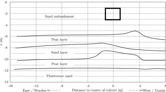
culvert (not to scale) . . . 8 2.3 Soil profile at the culvert. The position of the culvert is represented with a
square. Modified from (H¨olscher and Meijers, 2009) . . . 9 2.4 Height of ballast and position of the approach slabs from the GPR
mea-surements. Modified from (Coelho et al., 2011) . . . 10 2.5 Rail level measured during one maintenance period. Modified from (Coelho
et al., 2011) . . . 12 2.6 Evolution of settlement with days of the inner and outer rail at three
dif-ferent locations . . . 12 2.7 Voids measured under the sleepers. Modified from H¨olscher and Meijers
(2009) . . . 13 2.8 Photo of ballast sample taken from the track on top of the culvert . . . 13 2.9 Particle size distribution of two samples collected from the culvert site . . . 14 2.10 Photo of the monitored track section (May 2009) . . . 15 2.11 Position of geophones . . . 16 2.12 Vertical sleeper displacements during passage of an intercity doubledecker
train at 114km/h on the free track (G7), on top of the approach slab (G3) and on top of the culvert (G1). Modified from (Coelho et al., 2009) . . . 16 2.13 Vertical sleeper displacements at G7, G6, G5 and G3 . . . 17 2.14 Estimated settlement 7 months after the maintenance operation: (i)
au-tonomous settlement due to subgrade, (ii) ballast settlement under the inner rail and (iii) ballast settlement under the outer rail . . . 19
3.1 Strains during one cycle of compression load application. (a) - separation between permanent and resilient strains; (b) - non-linear elastic model . . . 22 3.2 Stress-strain diagram of a granular material under repeated loading
(Al-laart, 1992) . . . 23 3.3 Relative contributions of substructure to the settlement of the track (from (Selig
and Waters, 1994)). . . 25 3.4 Permanent strains in ballast from four triaxial tests with variable cyclic
amplitudes of loading (from Stewart (1986)).
σ1 - (variable) vertical stress;σ3 - (constant) horizontal stress . . . 26
4.2 General force-displacement behaviour of the springs . . . 38
4.3 Rail/sleeper system on iteration one of calculations . . . 39
4.4 Schematic longitudinal view of the train-track model . . . 44
4.5 Apparent dispersion curve of vertical motion at the surface . . . 46
4.6 Geometrical and mechanical parameters of the vehicles . . . 47
4.7 Force-displacement path of the springs . . . 49
4.8 Vertical measured level of the: (a) inner rail, (b) outer rail . . . 50
4.9 Force distribution at rest on the inner rail (a) and on the outer rail (b). Each circle corresponds to one sleeper. The dotted lines are scaled representations of the rail level . . . 51
4.10 Introduced voids under the hanging sleepers . . . 52
4.11 Displacements of sleepers G7 to G1 due to ICR passage . . . 53
4.12 Upward motion of the track after the passage of the wheels over the first trough before the culvert . . . 54
4.13 Maximum upward (top) and downward (bottom) displacements for sleeper located at G3 (x=−3.6m) depending on the friction damping . . . 54
4.14 Maximum upward (top) and downward (bottom) displacements depending on the location and the friction damping . . . 55
4.15 Force transmitted through half sleeper to the ballast, on a sleeper before the transition zone (dotted line) and on the sleeper located two sleepers before the culvert centre (full line) . . . 56
4.16 Transmissibility due to an ICR passage and an ICM passage considering the track level shown in Figure 4.8(b) and the hanging distances shown in Figure 4.10 . . . 56
4.17 Transmissibility considering a track level measured after a maintenance operation and a horizontal track level, both for an ICR passage and no voids under the sleepers . . . 57
4.18 Longitudinal view of the track, showing the possible flow of ballast in the transition zone . . . 58
5.1 Methodology for calculation of track level degradation . . . 63
5.2 Progression of settlement for three different values ofβ for constant loading amplitude (thin solid lines). Comparison with the settlement model of Shenton (dashed line) . . . 66
5.3 Example of an inverted cumulative histogram . . . 68
5.4 Settlement produced by load sequence presented in table 5.1. The vertical dashed line indicates the end of period 1 . . . 68
5.5 Settlement curves obtained with four different load paths (lines). Compar-ison with the results obtained by Stewart (circles and triangles) (Stewart, 1986). . . 68
5.9 Calculated and measured level of the inner (a) and outer (b) rail at three instants of time . . . 75 5.10 Level of the inner rail (solid line) and level of the top surface of the ballast
(dots) calculated at day 210 . . . 76 5.11 Measured and calculated voids under the sleepers. The measured voids
correspond to an average of values measured between day 196 and 210. . . . 76 5.12 Amplitude of the forces passing to the ballast at each sleeper of the model
caused by the passage of a LOC vehicle passing from left to right. Results obtained for the inner rail at day 210 . . . 77 5.13 Total settlement of ballast during the 210 days of the analysis. Results with
dynamic mass-spring model for the vehicles and with moving constant forces 78 5.14 Maximum downward displacements caused by the passage of an ICR vehicle
considering the initial level of the track, without voids under the sleepers. Results obtained with the non-linear model and with the linear model . . . 80 5.15 Amplitude of the forces passing to the ballast at each sleeper of the model
caused by the passage of an ICR vehicle. Results obtained for the inner rail at day 85 . . . 80 5.16 Total settlement of ballast during the 210 days of the analysis. Results with
non-linear stiffness model and with quasi-linear stiffness model . . . 81
6.1 Overview of 3-D model . . . 86 6.2 Railtrack system and ballast/soil system shown in the direction of the track 87 6.3 Railtrack finite element model . . . 87 6.4 TheEr−θ relationship . . . 91 6.5 Sleeper-ballast interaction viewed in longitudinal direction of the sleeper . . 93 6.6 Axis system for vertical contact . . . 94 6.7 Sleeper-ballast interaction viewed in transverse direction of the sleeper . . . 94 6.8 Replacing bottom layer with spring-damper system. 2D view . . . 96 6.9 Transmitting boundaries with dashpots . . . 96 6.10 External weight applied in Pegasus. 2D view in longitudinal direction of
the track . . . 98 6.11 Calculation steps in Pegasus . . . 99 6.12 Finite element meshes 1, 2 and 3 in longitudinal view . . . 100 6.13 Stress history due to two axles passage at 40 m/s. Coloured lines are
nu-merical results and black lines are analytical results (Boussinesq solution) . 101 6.14 Qualitative representation of the displacement field in a longitudinal view . 102 6.15 Displacements at surface of ballast under the rail . . . 102 6.16 Time history of resilient modulus at the ballast and sub-ballast layers.
6.21 Distribution of the resilient modulus (Er) in a transverse view, when the
wheel loads are passing over the sleeper . . . 107
6.22 Distribution of the resilient modulus (Er) in a longitudinal view, aligned with the rail (y=−0.75 m), when the first axle is passing over the central sleeper of the model (t= 0.2 s) . . . 107
6.23 Vertical dynamic displacements obtained in the ballast for the slow moving load case. Comparison between linear and non-linear results . . . 108
6.24 Effect of the constitutive model on the stress paths at the ballast and sub-ballast layers. Results determined at points located under the rail and under the loaded sleeper (x= 0 m, y = 0.75 m), for the slow moving load case. The black dashed line is the failure line . . . 109
6.25 Effect of the constitutive model on the stress paths at the ballast. Results determined at points located under the rail and between the sleepers (x= 0.212 m,y = 0.75 m), for the slow moving load case. The black dashed line is the failure line . . . 110
6.26 Maximum contact stress between the sleeper and the ballast . . . 111
6.27 Octahedral shear strain distribution in a longitudinal view, aligned with the rail, when the front axle is passing over the central sleeper of the model (t= 0.2 s) . . . 112
6.28 Octahedral shear strain distribution in a transverse view, at x= 0.2125 m, when the front axle is passing over the central sleeper of the model (t= 0.2 s)112 6.29 Vertical dynamic displacements obtained in the ballast for the fast moving load case. Comparison between linear and non-linear results . . . 114
6.30 Effect of the constitutive model on the stress paths at the ballast layer. Results determined at points located under the rail (x= 0 m, y= 0.75 m) for the fast moving load case. The black dashed line is the failure line . . . 114
6.31 Damping ratio implemented with the Rayleigh Damping Method . . . 117
6.32 Transverse view of models used for total size verification . . . 118
6.33 Longitudinal view of models used for total size verification . . . 119
6.34 Effect of model size on: (a) vertical displacements and (b) vertical stresses, calculated at surface of ballast and at interface between sand embankment and peat layer, under the rail at x= 0 m . . . 120
6.35 Vertical displacements calculated: (a) at the sleeper (x= 0 m,y= 1 m,z= 0.8 m) for three train loads travelling at 130 km/h and (b) at the ballast (x= 0 m, y = 0.75 m,z = 0.8 m) for the 72 kN wheel load, with decomposition of total displacements into part due to ballast & sub-ballast deformation and remaining part due to soil layers deformation . . . 121
6.36 The culvert model in longitudinal (xz) view . . . 122
6.37 The culvert model in transverse (yz) view. Cut at x= 0 m . . . 123
6.38 Sleeper-Ballast force distribution at rest . . . 124
6.42 Position of geophones . . . 126 6.43 Voids under the sleepers around the culvert box. Profile 1 are voids
cal-culated in Chapter 5 and profile 2 are voids determined from the dynamic measurements in Chapter 4 . . . 127 6.44 Transmissibility due to an ICR passage, obtained with the 3-D model
con-sidering the void profile 1 and 2, and with the 1-D model concon-sidering the void profile 2 . . . 128 6.45 Vertical displacements and p-q stresses at four points inside the ballast layer
(z= 0.65 m) and aligned with the inner rail (y =−0.75 m) considering the void profile 1 . . . 129 6.46 Normal stresses in the ballast inside the ballast layer (z= 0.65 m), aligned
with the inner rail (y =−0.75 m) considering the void profile 1 . . . 130 6.47 Displacement field (magnified 400 times) shown in a longitudinal view at
y =−0.75 m and at t = 0.273 s, when the two front wheels are over the first approach slab . . . 131 6.48 Dynamic displacements and stresses inx−zplane on three locations on top
of the approach slabs atz= 0 m, aligned with the inner rail aty=−0.75 m and considering the void profile 1 . . . 132 6.49 Time history of stresses in a face coplanar with the inclined slabs at x =
−3.6 m, aligned with the inner rail at y=−0.75 m . . . 133 6.50 Stress pathsdetermined at points located under the inner rail (y=−0.75 m),
immediately above the approach slabs at z =−0.1 m. The dashed line is the failure line determined withφ′c=40 . . . 133 6.51 Maximum vertical displacements in transverse alignments leveled with the
approach slabs (z=−0.2 m) at three longitudinal locations . . . 134 6.52 Three transverse views of the octahedral shear strain . . . 135
7.1 Model of the track used for the standard case . . . 141 7.2 Rail and sleepers displacements in standard case model. Load of 72 kN
moving at 120 km/h . . . 143 7.3 Track modulus of the standard case transition . . . 143 7.4 Transmissibility of the standard case transition . . . 144 7.5 Rail and sleepers displacements for case with soft railpads. Load of 72 kN
4.1 Parameters values of soil profile . . . 45 4.2 Parameters of the ICM and ICR vehicles . . . 47 4.3 Track parameters . . . 47 4.4 Average wheel load, train velocity and corresponding maximum downward
displacement on locations away from the transition zone (G7) and on top of the culvert (G1) . . . 48 4.5 Springs parameters . . . 48
5.1 Loading sequence with two periods . . . 67 5.2 Static wheel loads of the railway vehicles . . . 70 5.3 Parameters of the LOC and DD vehicles . . . 73 5.4 Traffic defined in terms of number of vehicles per unit of time, static wheel
loads and velocities of the railway vehicles . . . 73 5.5 Selected values for parameterγ, expressed in [mm] . . . 74 5.6 Equivalent stiffness of the linear springs . . . 79
6.1 Maximum size of finite elements . . . 100 6.2 Material properties of models with mesh-type 2 and 3 . . . 101 6.3 Material properties of ballast, sub-ballast, and sand layers . . . 105 6.4 Material parameters of soil profile . . . 116 6.5 Maximum vertical displacements measured at G7 and obtained with
nu-merical model . . . 121
7.1 Track properties of the standard case model . . . 142 7.2 Properties of the slab track . . . 164 7.3 Properties of the fill material . . . 165
Convention
a,A, α Scalar
a Vector
A Matrix
Subscript
aa Quantity referred to wheel-rail interaction
ad Quantity referred to damping
ae Quantity referred to deformation ag Quantity referred to gravity ai Quantity referred to inertia ard Quantity referred to the damper asp Quantity referred to the spring
as Quantity referred to the ballast-soil system at Quantity referred to the track system av Quantity referred to the vehicle system
Latin Symbols
a anda Accelerations
C Damping matrix
crd Visco-elastic damper constant
D Constitutive stiffness matrix
E Young’s modulus
Er Resilient modulus
EI Bending stiffness
h height of the void (also called gap) under the hanging sleepers
I Moment of inertia
K Stiffness matrix
K Bulk modulus
K0 Coefficient of lateral earth pressure
L Length
M Mass matrix
M Oedometer modulus
m Mass per unit length
Mf Inclination angle of failure line
N Number of applied load cycles
p Mean normal stress
q Deviatoric stress
∆S Maximum accumulated settlement between dynamic analyses
SN Settlement after N load cycles
Sb Settlement due to changes in the ballast and sub-ballast layers
Sr Settlement of the rail
Ssg Settlement due to changes in the subgrade
TR Transmissibility
t Time
u and u Displacements
uc Displacement at which the sleeper contacts the ballast
up Permanent deformation of the ballast
v and v Velocities
vp Velocity of primary body wave
vs Velocity of secondary body wave
Greek Symbols
δ Indentation
ǫs,r Recoverable shear strain
ǫv,r Recoverable volumetric strain
ǫi Principal strains (1 - major, 2 - intermediate, 3 - minor)
ǫN Total permanent strain after load cycle N
ǫi,r Recoverable strain in direction i
ǫij Strain tensor
γ Shear strain
γoct Octahedral shear strain
ν Poisson’s ratio
φc Critical state friction angle
ρ Volumetric mass
σi Principal stresses (1 - major, 2 - intermediate, 3 - minor)
σij Stress tensor
τ Shear stress
θ Sum of the principal stresses
θ0 Reference stress (100 kPa)
ǫ Vector form of the strain tensor
σ Vector form of the stress tensor
Abbreviations
1-D One-dimensional
2-D Two-dimensional
3-D Three-dimensional
BEM Boundary Element Method
CCP Triaxial test with constant confining pressure
FDM Finite Difference Method
FEM Finite Element Method
GPR Ground Penetration Radar
GPS Global positioning system
ICM Railway vehicle - Intercity trainunit ICR Railway vehicle - Intercity carriage
IEM Infinite Element Method
Introduction
1.1
Background to the study
Railways are recognized as the most reliable, safe and energy efficient means of transport for passengers and goods. In an era of increasing environmental concern, railway transport is also the most sustainable choice, with the lowest CO2emissions per km.ton transported. With this in mind, the railway sector has been the subject of renewed interest and rapid development in the last few decades. The expansion of the railway network is taking place mainly in China, Europe and Japan (Okada, 2007; EU, 2001; Takatsu, 2007).
One of the main disadvantages of railway transport is the high cost of construction and maintenance, when compared to other modes of transport. Furthermore, the increase in speed, axle-loads and traffic has led to higher-rates of degradation of the ballasted railway tracks (Schmitt, 2006; L´opez-Pita et al., 2007). As so, a considerable effort is necessary for maintenance of the tracks, with corresponding increase in costs for the infrastructure managers. According to Schmitt (2006), 40-50% of these costs are spent to maintain the quality of the track geometry. The main cause for the loss of track geometry is deformation and densification of the ballast layer, representing 75% of the total track position maintenance (Selig and Waters, 1994; Esveld, 2001; Zhai et al., 2004). The seek for improved design solutions for railway tracks, keeping the maintenance costs at reasonable and competitive level, is thus the essential objective of the ongoing research on railways.
which the track geometry degrades on these transition zones is frequently higher than on the normal free track, leading to higher maintenance frequency and sometimes speed re-strictions (Dahlberg, 2003; Li and Davis, 2005; Sasaoka and Davis, 2005; L´opez-Pita et al., 2007). According to L´opez-Pita et al. (2007) the frequency of maintenance at transitions in the Spanish railway line is three times that of normal plain track. In the Netherlands, where this problem is aggravated by the existence of soft soil conditions, it was found that the incidence is 4-8 times higher (H¨olscher and Meijers, 2007). Therefore, additional research on railway transitions will allow the development of optimized maintenance pro-cedures, and improved transition zones solutions for new railway lines or for the up-grade of existing ones.
1.2
Aim of the research
According to an extensive monitoring campaign performed in the US (Li and Davis, 2005), the poor performance of transition zones is significantly dictated by degradation mech-anisms occurring in the ballast. The principal aim of this research is thus to improve knowledge on the ballast behaviour at transition zones, seeking a clarification of the causes responsible for the change of geometry of ballasted tracks on these areas, and to answer the question which mechanisms are responsible for the observed increased degradation.
At transitions, the dynamic loading on the ballast is highly influenced by the inhomoge-neous nature of the support, which includes changes of the support stiffness and, possibly, voids under the sleepers. These aspects may evolve in time, with the accumulation of settlement at transitions, and therefore their influence on the long-term response of the track will also change in time. This study pursuits the development of a novel method suitable to predict the long-term behaviour of transition zones, considering the coupling between the dynamic response and the long-term behaviour.
This work also seeks the development of novel computer models adequate to analyze the dynamic behaviour of transition zones. The dynamic response of the track at transition zones is particularly affected by non-linear aspects. These non-linear aspects include the loss of contact between the sleepers and the ballast, and the non-linear constitutive behaviour of the ballast (Dahlberg, 2003). Another aim of this research is thus to analyze the importance of the consideration of these non-linear aspects in representative models, and how these non-linear aspects influence the obtained numerical response.
1.3
Outline of the thesis
This thesis is composed of eight Chapters. In Chapter 2 of the thesis, the study starts by describing the usual problems associated with transition zones, and by presenting field measurements performed at one typical railway transition. The data collected in the field yielded a better understanding of frequent problems occurring in transition zones, and also allowed for a comprehensive quantification of its dynamic and long-term response. For this reason, the case described in this Chapter is the central case-study of this work. At the end of Chapter 2, a series of research questions concerning this case-study are formulated.
In Chapter 3, the mathematical models for railway tracks and ballast behaviour are re-viewed, and important aspects to be considered in the models used within this work are identified.
Chapter 4 presents a one-dimensional train-track dynamic numerical model, incorporating non-linear aspects. This model is validated with the measurements given in Chapter 2, and some of the research questions formulated at the end of Chapter 2 are answered based on the numerical simulations.
Chapter 5 presents a methodology to estimate the loss of the vertical geometry of the track with time. For this, the dynamic model developed in Chapter 4 is coupled with a newly developed mathematical model to estimate the vertical settlement of the ballast, also presented in Chapter 5. The validation of the method and the settlement model is made with the long-term measurements given in Chapter 2. With the presented methodology, the importance of the coupling between the dynamic loading from the trains and the long-term response of the track is analyzed.
Results from Chapter 5 point to the need for additional dynamic simulations using three-dimensional models. Accordingly, a three-three-dimensional numerical model for the dynamic response of transition zones is developed and presented in Chapter 6. In this Chapter, the importance of the non-linear constitutive behaviour of the ballast on its dynamic response is also investigated, and the 3-D model is applied to study the standard transition case of the field measurements.
the support, therefore representing the case of a railway transition, and the corresponding solution is obtained with analytical methods.
Railway Transition Zones.
Problem Description
2.1
Overview
Transition zones in railway tracks are built to mitigate the impact caused by structural discontinuities along the track. These discontinuities may be bridge approaches, passages over culverts, at road and rail crossings, ends of tunnels, or passages from slab tracks to ballasted tracks. Such places frequently show accelerated track geometry degradation and increased wear and tear on track and vehicle components. This leads to poor ride quality and sometimes speed restrictions. As a consequence, the maintenance incidence on track discontinuities may be three to eight times higher than that in normal plain track, increasing costs and decreasing the availability of the track (Kerr and Moroney, 1993; Kerr and Bathurst, 2001; Li and Davis, 2005; Read and Li, 2006; L´opez-Pita et al., 2007; H¨olscher and Meijers, 2007).
Two main causes are generally referred for the observed increased degradation at track discontinuities (Shenton, 1985; Hunt, 1997; Kerr and Bathurst, 2001; Li and Davis, 2005; Lundqvist et al., 2006):
(ii) On transitions, the ballasted approach section may inherently settles more than the section on top of the stiff structure, as the former is frequently built over embank-ments and the stiff structure is usually free of settleembank-ments. This, again, leads to differential settlements.
The uneven settlements occurring at these locations frequently lead to unsupported sleep-ers (also called hanging sleepsleep-ers). These are sleepsleep-ers suspended by the rails in the unloaded condition and thus with a gap between the sleeper and the ballast bed. Figure 2.1 shows the existence of hanging sleepers, which may appear in the vicinity of stiffer structures supporting the track. The existence of unsupported sleepers lead to impact loading on the track and thus to accelerated track damage, making it another cause for the observed increased degradation (Hunt, 1997; Augustin et al., 2003; Lundqvist and Dahlberg, 2005; Zhang et al., 2008).
Figure 2.1: Structural discontinuity in the track
Briaud et al. (1997) refers to other causes for the differential settlements at bridge ap-proaches, which include geotechnical defects, such as insufficient compaction and consoli-dation of the fill and embankment, poor drainage conditions, compression of natural soil due to embankment load, among others.
A number of different solutions for transition zones have been proposed or used. These transitions are built to smooth the stiffness variation between the “soft” approach section and the “stiff” section on top of the structure. Transitions based on smoothing the stiffness variation on the “soft” side (Kerr and Moroney, 1993; Li and Davis, 2005; Read and Li, 2006) include the use of oversized sleepers, variable spaced sleepers, underlayments of hot-mix-asphalt or of geotextiles or of soil-cement, additional rails, approach slabs, among others. Transitions based on lowering the stiffness on the “stiff” section (Kerr and Moroney, 1993; Kerr and Bathurst, 2001; Sasaoka and Davis, 2005; Read and Li, 2006; Li et al., 2010) include the use of soft railpads, under sleeper pads, plastic sleepers or ballast mats. According to Li and Davis (2005), transition zones must address the specific stiffness issues of the correspondent track discontinuities in order to be effectives.
2.2
Field measurements on a railway transition
Experimental investigations on the behaviour of structures are important, not only because they allow for a good understanding of the physical phenomena under study, but also because they give data for the validation of representative models. As mentioned above, field measurements in transitions of railways are scarce. In the Netherlands, a monitoring programme was defined in order to improve knowledge on the behaviour of transition zones, comprising both short-term and long-term measurements. The field measurements were performed between 2008 and 2009, in a culvert box transition, located in a region with soft soils. The author had the opportunity to closely follow these field measurements, with a small contribution in the field. The collected data played an important role in the development and validation of the models presented in this work. Therefore, the data needed in Chapters 4 to 6, for validation of the models, will be presented next. These field measurements are extensively described in (H¨olscher and Meijers, 2009; Coelho, 2011).
2.2.1 Case description
and a longitudinal view of the culvert. Figure 2.2-a shows only the two newer tracks. The measurements were concentrated on the outer track (right-hand side in figure 2.2-a). In these two tracks, the trains travel from East to West.
1.0m
2.0m
4.0m 2.0m 4.0m
a)
b) Concrete culvert
Inner rail Outer rail
Ballast Sand
Peat/Clay
Sand
West East
culvert approach slabs Ballast
Track
Sand embankment
Figure 2.2: Transverse view (a) and longitudinal view (b) of the track passing over the culvert (not to scale)
Figure 2.3 shows the soil profile at the culvert. This profile was obtained based on CPT’s, VSPT’s and Ground Penetration Radar (GPR) measurements (H¨olscher and Meijers, 2009). The reference for the vertical axis is placed at the top surface of the ballast.
West / Gouda Distance to centre of culvert [m]
8 4
-16 -12 -8 -4 0
East / Worden -14
-12 -10 -8 -6 -4 -2 0
z[
m
]
Peat layer
Peat layer Sand layer Sand embankment
Pleistocene sand
Figure 2.3: Soil profile at the culvert. The position of the culvert is represented with a square. Modified from (H¨olscher and Meijers, 2009)
According to the VSPT’s (H¨olscher and Meijers, 2009), the shear wave velocity of the peat is around 50 m/s for the layer above the intermediate sand layer and around 80 m/s for the layer under this sand layer. The shear wave velocity of the intermediate sand layer is about 150 m/s and that of the pleistocene sand can be estimated to be slightly higher. At the embankment, the shear wave velocity could not be reliably measured and the CPT’s showed significant variations in terms of tip resistance. This indicates a heterogeneous nature of the embankment.
z[
m
]
Distance to the center of the culvert [m]
-25 -20 -15 -10 -5 0 5 10 15 20 25
Ballast Approach slab -0.4
-0.2 0
0.2 0.4 0.6 0.8 1.0 1.2 1.4 1.6
Figure 2.4: Height of ballast and position of the approach slabs from the GPR measurements. Modified from (Coelho et al., 2011)
2.2.2 Long-term behaviour
The long-term behaviour of the track was measured during one maintenance period (nine months). The measurements here presented include the periodic levelling of the track and the measurements of the voids under the sleepers.
Settlement of subgrade and approach slabs
The settlement of the free track embankment was estimated from the periodic measure-ment of the level of four concrete pylons, founded on the embankmeasure-ment and supporting the catenaries at this site (H¨olscher and Meijers, 2009). It was found that the settlement of these pylons can be approximately represented by a linear function of time, with an average settlement rate of 1mm/month, relative to the culvert. This settlement may be considered as an indication of the settlement of the subsoil, supporting the embankment. This settlement is mainly due to consolidation of the peat layer (Coelho, 2011).
present value of 18.5% (H¨olscher and Meijers, 2009).
Vertical motion of the track
The long-term vertical motion of the track was measured on top of each rail along one main-tenance period. These levelling operations were made with high-precision topographical equipment, based on the Global Positioning System (GPS). The precision of the equipment was 0.5 mm. The level was measured above each sleeper, spaced 0.6 m. Figure 2.5 shows the spatial evolution of the level of the inner rail (as defined in Figure 2.2-a). The first levelling on 7thOctober 2008 was performed a few hours after the maintenance operation. The figure also shows the position of the culvert and approach slabs. Figure 2.6 shows the time evolution of the inner and outer rail level in three different locations: on top of the culvert, on the free track to the East (x = −12.6m) and on the free track to the West (x= +12.6m). In this figure, the vertical position is relative to the initial position, measured on 7th October.
Several observations are made looking at Figures 2.5 and 2.6:
- The track presents an up-and-down profile when passing over the culvert. The length of this bump is 10 to 20 m;
- The settlement is faster initially, right after the maintenance operation;
- After day 51 (27th of November), the settlement is negligible on top of the culvert and evolves approximately linearly with time at the embankment areas;
- The initial settlement is higher on the outer rail compared to the inner rail;
- The initial settlement is higher on the embankment areas compared to the initial settlement on top of the culvert;
- The initial settlement is higher on the West side of the culvert compared to the East side.
Voids under the sleepers
-15 -10 -5 0 5 10 15 -40
-35 -30 -25 -20 -15 -10 -5 0 5
Distance from center of culvert [m]
Rail Level [mm]
7 Oct 2008 27 Nov 2008 21 Jan 2009 27 Fev 2009 18 Mar 2009 21 Apr 2009 5 May 2009
Figure 2.5: Rail level measured during one maintenance period. Modified from (Coelho et al., 2011)
0 50 100 150 200
−16 −14 −12 −10 −8 −6 −4 −2 0
Days
Rail settlement [mm]
Top Culv. − inner Top Culv. − outer Emb. East − inner Emb. East − outer Emb. West − inner Emb. West − outer
Figure 2.6: Evolution of settlement with days of the inner and outer rail at three different locations
values (vertical lines). The scatter is significant during the one month survey. From the figure, it can be seen that there is a significant amount of voids under the sleepers located above the approach slabs (between -5m to -1m and 1m to 5m) and that on top of the culvert, as expected, the sleeper soffit is in contact with the ballast.
Ballast behaviour
−10 −8 −6 −4 −2 0 2 4 6 8 10 0
5
10
15
Distance from center of culvert [m]
Voids height[mm]
Figure 2.7: Voids measured under the sleepers. Modified from H¨olscher and Meijers (2009)
Figure 2.8: Photo of ballast sample taken from the track on top of the culvert
ballast particles, particle size determination and Los Angeles abrasion tests. Figure 2.8 shows one photo of part of a ballast sample.
The petrographical examination, including microscopic analysis, concluded that the ballast is composed, at least, by three different types of rocks: basalt, gneiss and rhyolites. These rocks have different mechanical properties in terms of strength. The fact that most ballast in the Netherlands is imported and that several re-ballast operations were done since initial construction can explain the existence of three types of rocks in the ballast.
0 10 20 30 40 50 60 70 80 90 100
0,50 5,00 50,00
Cum
m
ul
at
iv
e w
ei
ght
p
assi
ng
(%
)
Particle size (mm)
Figure 2.9: Particle size distribution of two samples collected from the culvert site
It can be seen in Figure 2.9 that the particle size distribution of the collected ballast lies outside the admissible limits imposed by the norm. The ballast particles sizes are generally smaller than they should be. Disregarding the hypothesis that the ballast was placed in the track with inadequate granulometry, it may be stated that the particle breakage at the culvert site is significant. Visual inspection of the collected ballast has also identified fresh cuts in some ballast particles confirming this assumption. This particles breakage alter the mechanical properties of the ballast, worsen its drainage capacity and contribute to the track geometry degradation.
2.2.3 Short-term behaviour
Train-induced track vibrations were measured using geophones, accelerometers and one high-speed camera. These measurements were done in May 2008 and May 2009, during regular train passages. Figure 2.10 shows a photo of the short-term measurements appa-ratus. The complete set up for the dynamic measurements is described in (H¨olscher and Meijers, 2009; Coelho et al., 2011). Here only part of the track motion measurements in May 2008 are briefly presented.
Figure 2.10: Photo of the monitored track section (May 2009)
The displacements measured by geophones G7, G3 and G1 during one train passage at 114km/h are shown in Figure 2.12. From this figure, it appears that the upward mo-tion has about the same magnitude as the downward momo-tion. However, this is in fact a consequence of the filter and integration procedure, necessary to transform velocities to displacements (Bowness et al., 2007). From comparison with the displacements directly measured with the high-speed camera, it was concluded that a downward drift of the dis-placements obtained with the geophones is necessary, in order to represent the real upward and downward motion of the sleepers (Coelho et al., 2009).
Comparing the displacements above the free track (G7) and above the culvert (G1), it can be seen that the peak-to-peak displacements differ by a factor of 2. The stiffness on top of the culvert is higher, as expected. Over the approach slab, there should be a gradual transition, in terms of displacements and stiffness, between the free track and the culvert (Kerr and Moroney, 1993; Esveld, 2001). However, the measured displacement amplitudes on location G3 were much higher than at G7 and G1.
G7 G6
Direction of trains
G1 G2
G3 G4 G5
Figure 2.11: Position of geophones
4 5 6 7 8 9 10 11 12 13 14
−5 0 5
Time [s]
Displacements [mm]
4 5 6 7 8 9 10 11 12 13 14
−5 0 5
Time [s]
Displacements [mm]
4 5 6 7 8 9 10 11 12 13 14
−5 0 5
Time [s]
Displacements [mm]
G7
G3
G1
7 7.5 8 8.5 9 9.5 10 −6
−4 −2 0 2
Time [s]
Displacements [mm]
G7 G6 G5 G3
Spike
Figure 2.13: Vertical sleeper displacements at G7, G6, G5 and G3
2.2.4 Interpretation and discussion
The settlement of the embankment was found to evolve approximately linearly with time. The settlement of the embankment results from permanent deformations in the soft layers of peat and in the sand layer forming the embankment itself. These settlements evolve non-linearly from the time the track was built. However, between two successive maintenance operations, after some years of service operation, the settlement of the subgrade can be approximated by a linear function of time (Shenton, 1985; Sato, 1995).
The measurements have shown that the tips of the approach slabs are settling at an higher rate, relative to the settlement of the embankment. The mechanism causing the higher settlement rate of the approach slabs may be a flow of sand from under the slab to under the culvert, combined with higher densification caused by a concentration of stresses at the free ends of the slabs, motivated by the existence of a voided region under the approach slabs, close to the culvert vertical wall (H¨olscher and Meijers, 2009).
re-ballasting operations required for the upkeep of the track.
According to literature, the rapid settlement measured at the rail level during the first period after maintenance is mainly caused by densification of the ballast (Sato, 1995; Dahlberg, 2001). The lift of the track is performed with tamping operations which basically consists on lifting the sleepers to a prescribed level, after which steel tines are inserted in the ballast, vibrating and squeezing the underlying ballast particles to fill the voids under the sleepers (Suiker et al., 2005). This operation destroys the previous stable particle arrangement of the ballast, loosens the ballast, decreases its strength and stiffness and causes particle breakage (Esveld, 2001; Indraratna et al., 1998; Anderson and Key, 2000; Suiker et al., 2005). Therefore, as soon as traffic is reestablished, the densification of ballast restarts, by means of particle rearrangements, reducing its void ratio and augmenting its stiffness, until the ballast particles find a new stable configuration.
The higher initial settlement at the outer rail, compared to the inner rail, may be explained by the fact that the outer rail is closer to the ballast slope. This implies lower confinement of the ballast located under the outer rail, compared to the ballast under the inner rail, leading to higher rates of densification of the ballast (Lackenby et al., 2007). Moreover, it was visually observed that the inclination of the ballast slope, initially high after the maintenance, rapidly flattens as ballast reestablishes a stable configuration. This indicates a flow of ballast in the lateral horizontal direction, which also contributes for a global lateral rotation of the track towards the outside.
The initial settlement of ballast is smaller on top of the culvert than at the embankment areas. This is explained by the existence of a rigid surface under the ballast on top of the culvert. According to Saussine et al. (2006), who performed numerical simulations using the discrete element method, high stiffness of the underlayers implies a strong contact force network, more compactness of the pack, and less movement of particles under the sleepers, whereas in case of more flexible underlayers, the force intensity between particles is lower, which facilitates the circulation of particles under the sleepers. Furthermore, the initial lower settlement of ballast on top of the culvert can also be attributable to the fact that the existence of a rigid surface under the ballast, as is the culvert, will yield an higher efficiency during the compaction of the ballast layer, performed during the maintenance operation, immediately after the lift and tamping of the track (Faure, 1982).
sub-ballast layers. Therefore, an expression as
Sr.i+hi=Sb.i+Ssg.i (2.1)
is possible for sleeper i, where Sr represents the settlement of the rail, h the height of the void under the sleeper, Sb represents the settlement due to changes in the ballast and sub-ballast layers, and Ssg the settlement of the subgrade. Using Equation (2.1), the settlement due to changes in the ballast and sub-ballast layer, Sb, at the culvert site can be estimated. For this, the quantityhiis estimated for all sleepers, interpolating from the average results shown in Figure 2.7, and assuming no voids under the sleepers above the culvert, and no voids under the sleepers away from the transition zones.
Figure 2.14 shows the estimated settlement, after 7 months of service operation. The figure presents the assumed subgrade settlement, Ssg, which includes the effect caused by the rotation of the approach slabs, and the settlement of the ballast, Sb, determined with Equation (2.1), under the inner rail and under the outer rail. From Figure 2.14, it can be seen that the ballast settlement (Sb) presents significant fluctuations on the transition zones. This settlement is maximum on locations -1.8 m and 1.8 m, which are locations on top of the approach slabs but close to the culvert. Figure 2.14 shows that the settlement on the transition zones (equal to Sb+Ssg) is caused by two factors: a rotation of the approach slabs, motivated by the subgrade settlement, which is dominant between 3 m to 6.6 m away from the culvert center, and increased localized permanent deformations of the ballast layer, which is dominant between 1.2 m to 3.0 m away from the culvert center.
−15 −10 −5 0 5 10 15
0
5
10
15
Distance from center of culvert [m]
Settlement [mm]
Autonomous Ballast inner Ballast outer
Sbinner
Sb outer
Ssg
Figure 2.14: Estimated settlement 7 months after the maintenance operation: (i) autonomous settlement due to subgrade, (ii) ballast settlement under the inner rail and (iii) ballast settlement under the outer rail
the transition, or above the culvert. The reason for these higher displacements seems to be the existence of consecutive hanging sleepers on both sides of the culvert. Figure 2.5 shows that the track level, starting from the culvert centre to each side, is similar to that of a uniformly loaded cantilever beam: this is a preliminary indication for the existence of consecutive hanging sleepers. Furthermore, the increase in downward displacements evidenced in Figure 2.13, follows approximately the void profile shown in Figure 2.7.
2.2.5 Research questions
The monitoring campaign has given valuable data that allowed for a comprehensive un-derstanding of the short-term and long-term behaviour of a culvert transition. However, there are still some aspects requiring further analyses and clarification. Some of these aspects are:
(i) how many consecutive sleepers are hanging, and what is the amount of void under each hanging sleeper?
(ii) what is the reason for the upward displacement spike of the sleepers located at the transition zones?
(iii) what is the force transmitted through each sleeper to the underlying ballast in the transition area?
(iv) what are the causes for the observed increased settlement of the ballast above the approach slabs, as evidenced in Figure 2.14?
State-of-the-Art on Modelling of
Ballast and Railway Tracks
The existing technical literature is reviewed with emphasis on two main topics: the be-haviour of ballast under dynamic loading, and mathematical models representative of railway tracks loaded by moving trains. Recent reviews describing comprehensively these issues can be found in Ionescu (2004); Lim (2004); Indraratna and Salim (2005) for the mechanics of ballast, and in Beskou and Theodorakopoulos (2011) for models representing railway tracks.
3.1
The mechanical behaviour of ballast
3.1.1 Resilient behaviour
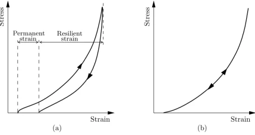
The deformation of ballast produced during one cycle of railway-type loading can be sepa-rated in a resilient (recoverable) part and a permanent part, as depicted in Figure 3.1 (a). Except for the initial phase of loading, while ballast is in a loose state, the deformation of ballast during train loading is essentially recoverable (Uzan, 1985; Fortunato, 2005). Due to this, the non-elastic behaviour of ballast is frequently neglected on constitutive models, assuming the material presents an elastic response, as shown in Figure 3.1 (b).
Strain
Resilient
Str
ess
(a)
Strain (b)
Str
ess
strain Permanent
strain
Figure 3.1: Strains during one cycle of compression load application. (a) - separation between permanent and resilient strains; (b) - non-linear elastic model
The resilient behaviour of ballast is highly governed by deformation of the ballast par-ticles under compression loads. At a microscopic level, when two (sphere) parpar-ticles are gradually pressed against each other, the contact surface increases, and the rate of change of the contact stress decreases, leading to higher stiffness at higher level of applied pres-sure (Timoshenko, 1915). This partly explains the non-linear stress-strain path of ballast under compression loads, with the stiffness increasing with the stress level, as can be seen in Figure 3.1 (b).
The resilient nature of ballast is commonly quantified by the resilient modulus,Erand the Poisson’s ratio, ν, which for repeated load triaxial tests with constant confining pressure (CCP) are defined as,
Er=
∆(σ1−σ3)
ǫ1,r
(3.1)
ν=−ǫ3,r
ǫ1,r
where σ1 and σ3 are the major and minor principal stresses, and ǫ1,r and ǫ3,r are the major and minor recoverable strains, respectively. The resilient modulus is the (non-linear) equivalent to the Young’s modulus of the traditional theory of linear elasticity.
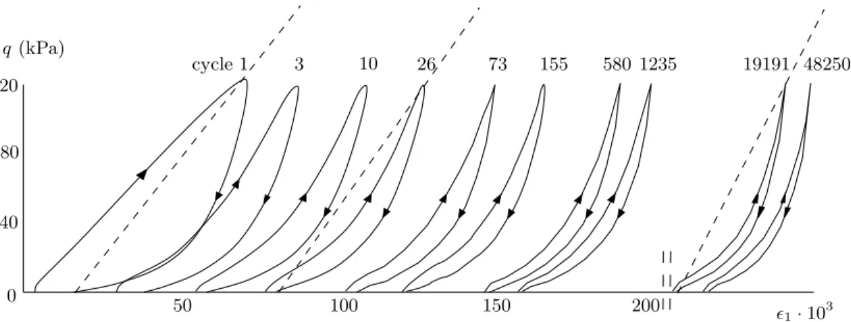
The resilient modulus Er increases considerably with the stress level, mainly with the confining pressure and the sum of principal stresses (Hicks, 1970; Uzan, 1985; Sweere, 1990; Kolisoja, 1997). The modulus Er also increases with the number of applied load cycles, N, mainly during the first cycles (Allen, 1973; Kedhr, 1985). After the completion of a small number of cycles (typically less than 1000 cycles), the value of Er still increases with N, but at a very small rate (Lackenby et al., 2007). Figure 3.2 represents a typical stress-strain diagram of a granular material under repeated loading. The resilient modulus at the first load cycle, at the 26th cycle, and at the final stage of the test, is the inclination of the corresponding dashed lines in the figure. The figure also shows the stiffening of the material with the increase in stress and the stabilization of the stress-strain path for increasing N.
0
cycle 1 3 26 73 155 580 1235 19191 48250
200 150
100 50
q(kPa)
10
ǫ1·103 120
80
40
Figure 3.2: Stress-strain diagram of a granular material under repeated loading (Allaart, 1992)
The most widely used model to describe the non-linear resilient nature of unbound granular materials is the K−θ model (Brown and Pell, 1967; Hicks, 1970; Hicks and Monismith, 1972). This model was developed to describe the results of CCP tests and expresses the dependency of the resilient modulus on the sum of the principal stresses, according to:
Er=K1
θ θ0
K2
(3.3)
According to Correia et al. (1999), when, in the end of the 70’s, more evolved triaxial tests with variable confining pressure (VCP) were performed to better represent the in situ loading conditions, it was seen that the resilient modulus depends not only on the sum of the principal stresses, θ, but also on the stress path, or the stress ratio (p/q) and that the Poisson’s ratio is not a constant and varies with the applied stresses (Brown and Hyde, 1975; Boyce, 1980; Sweere, 1990; Lackenby et al., 2007).
For that reason, Boyce (1980) proposed a different non-linear elastic model to describe the behaviour of granular materials under repeated loading. Instead of using the resilient modulus and the Poisson’s ratio to characterize the stress-strain relationship, Boyce uses a different approach, based on the bulk and shear moduli:
p=K ǫv,r (3.4)
q= 3 G ǫs,r (3.5)
where K is the bulk modulus, G is the shear modulus, p is the mean normal stress, q
is the shear or deviatoric stress, ǫv,r is the recoverable volumetric strain and ǫs,r is the recoverable shear strain. According to Brown and Hyde (1975), the separation of stresses and strains into volumetric and shear components gives a better description of the elastic behaviour of granular materials. In triaxial tests, where σ2 =σ3 and ǫ2=ǫ3, these stress and strain quantities are defined according to:
p= 1/3 (σ1+ 2σ3)
q =σ1−σ3
ǫv,r =ǫ1,r+ 2ǫ3,r
ǫs,r= 2/3 (ǫ1,r−ǫ3,r)
In the model of Boyce, the stress dependent values of K and Gare determined according to:
K =K1
p p0
1−n
· 1
1−pq22β
(3.6)
G=G1
p p0
1−n
(3.7)
with
β = K1(1−n) 6G1
stress value. The term 1−q 2
p2β, included in Equation (3.6), was derived so that the model preserves elasticity, which also means that no strain energy disappears for any chosen stress-strain path (Timoshenko and Goodier, 1970; Allaart, 1992). According to Correia et al. (1999), the Boyce model is superior to the K-θ model in predicting the non-linear behaviour of granular materials in VCP tests, with coefficients of correlation ranging between 0.6 and 0.9.
Other models derived from the Boyce model are available in the literature. For example, the contour model presented by Brown and Pappin (1981) extends the three-parameter model of Boyce to a five or even six parameter model. This model is able to predict test results very well, but it can be shown that this model is no longer entirely elastic (Allaart, 1992).
3.1.2 Settlement of ballast
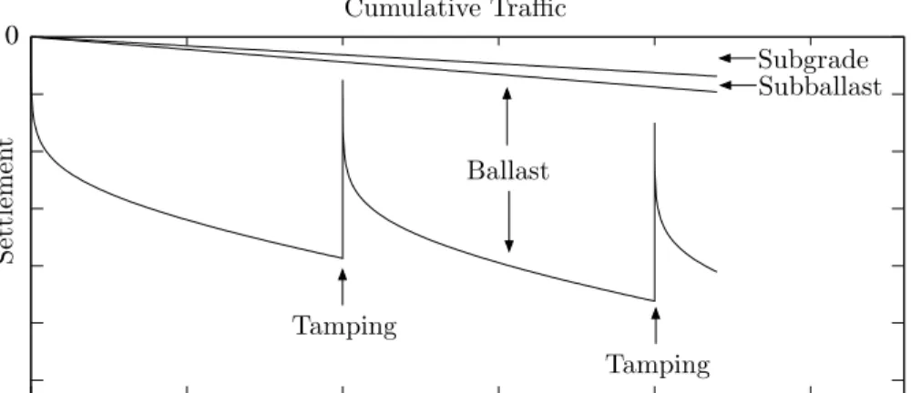
The degradation of the track geometry is due to settlements on the supporting layers of ballast, sub-ballast and subgrade. In regular tracks founded on good subgrade, the main contribution to track settlement is from the ballast, as can be seen in Figure 3.3, whereas the subgrade settlement is only significant during the early life of the track (Shenton, 1985).
0
Subballast
Settlemen
t
Ballast Cumulative Traffic
Tamping
Tamping
Subgrade
Figure 3.3: Relative contributions of substructure to the settlement of the track (from (Selig and Waters, 1994)).
Figure 3.4 shows results of cyclic triaxial tests on ballast performed by Stewart (1986). Four stress paths are shown where the loading amplitude changes at every 1000 load cycles. The loading was applied at 1Hz frequency varying from a constant minimum of 21kPa (coincident with the horizontal confining stress) to the following vertical amplitudes: 42kPa (A), 64kPa (B), 86kPa (C) or 107kPa (D). The stress paths are defined in the figure. It can be seen that when the loading amplitude increases above any previously applied value, the permanent deformation increases immediately, approaching asymptotically a new value with increasing number of cycles. According to these tests, the final permanent deformation does not depend on the sequence of loading. It can also be seen that the settlement rate decreases with an increasing number of load cycles, if the loading amplitude remains constant.
OD-OA-OB-OC
1000
0 3000 4000
Number of Cycles, N 0.2
0 1.0
0.8
0.6
0.4
2000
P
ermanen
t
V
ertical
S
train,
ǫN
,%
σ3c= 21kP a
OB-OC-OD-OA OA-OB-OC-OD
OC-OD-OA-OB
Figure 3.4: Permanent strains in ballast from four triaxial tests with variable cyclic amplitudes of loading (from Stewart (1986)).
σ1 - (variable) vertical stress;σ3- (constant) horizontal stress
Other factors influencing ballast behaviour are the minimum load caused by the unloaded track weight and impact loads on the ballast. The former is beneficial regarding the permanent deformation, by preventing dilatant behaviour and flow of ballast under cyclic loading (Baessler and Ruecker, 2003; Augustin et al., 2003; Lackenby et al., 2007). Impact loads, on the other hand, will increase permanent deformation on the ballast (Baessler and Ruecker, 2003).
Prob-ably the most important mechanism is compaction, where the packing assembly of ballast is compressed due to gradual particle rearrangements (Sato, 1995; Dahlberg, 2003). This mechanism is dominant when ballast is first loaded, after the tamping operations. The second mechanism is the flow of ballast particles on lateral and longitudinal direction, especially from under the sleepers. Sato (Sato, 1995) considers this to develop linearly with the accumulation of traffic. The flow of ballast occurs in cases where the ballast is poorly confined, when suspended sleepers impact the ballast (Baessler and Ruecker, 2003) or when high lateral loads are transmitted by the trains to the sleepers. Other degradation mechanisms include breakage and abrasion of ballast particles (Lim, 2004; Sekine et al., 2005; Lackenby et al., 2007), the penetration of finer particles belonging to sub-layers on the ballast layer or the jumping of ballast particles caused by high dynamic action (Sato, 1995; Baessler and Ruecker, 2003).
Existing models
Available railway settlement models include the logarithmic model (ORE, 1970; Alva-Hurtado and Selig, 1981), the Shenton model (Shenton, 1985), the Sato model (Sato, 1995) and the Hettler model (Mauer, 1995). Dahlberg (2001) presents a critical review of some of the most important models, including these ones. Common features are:
(i) the models are empirically based;
(ii) the track settlement is characterized by two phases: an initial phase of rapid settle-ment after tamping followed by a phase where the settlesettle-ment rate is more or less constant with time (or number of cycles);
(iii) the loading of the track is determined by the number of loading cycles and/or passed tonnage;
(iv) the loading characteristics are assumed to be constant in time.
The logarithmic model states that
ǫN =ǫ1(1 +C log(N)) (3.8)
Through experiments and experience in Japan, Sato states that the accumulated settle-ment of the ballast may be determined from:
SN =γ(1−e−αN) +βN (3.9)
where N is the number of load cycles, and α, β and γ are parameters. In these two models, no distinction is made between loadings of varying magnitudes. Their application is therefore limited to cases where the loading magnitudes are approximately constant in time.
Based on available field data from world wide sources, Shenton stated that the logarithmic model may underestimate the settlement for a large number of cycles and that a preferable model is:
SN =Ks
Aeq 20
K1N0.2+K2N (3.10)
whereSN is the total settlement, Aeq the equivalent axle load,Ks a factor function of the sleeper type and size, ballast type and thickness, and the subgrade,K1 a factor function of the lift given to the track during maintenance and K2 a constant value. According to Shenton, the first part represents the ballast settlement immediately after tamping, predominating up to one million load cycles, and the second part the residual settlement which occurs in the deeper ballast and foundation. The proposed formula to determine the equivalent axle load is:
Aeq =
5
N
n=1A5n
N (3.11)
whereAnis the axle load passing at load cycle n.
Hettler presents a model, based on the logarithmic model (Eq. (3.8)):
SN =s Feq1.6 (1 +C log(N)) (3.12)
whereFeqis the equivalent sleeper-ballast force andsandCare model parameters. Hettler defined the equivalent sleeper-ballast force as the mean value of the applied loads:
Feq = 1
N
N
n=1
Fn (3.13)
is much less influenced by changes in Fn.
Mathematical schemes for the logarithmic based models, (3.8) and (3.12), with variable loading amplitudes can be found in (Stewart, 1986; Ford, 1995; Mauer, 1995). These methods are only practical for cases with a limited number of load changes, between phases of constant loading amplitudes.
The loading history is not treated accurately with the models presented above. Therefore, they are hardly suited to study cases where the amplitudes of loading may continuously change. This is the case in transition zones founded on soft soils. In Chapter 5, a novel settlement model to address this problem will be presented.
3.2
Mathematical models for railway tracks
3.2.1 Overview
The first mathematical models developed to determine the dynamic response of railtrack-like structures were one-dimensional. These models were generally composed of a beam, representing the rail, laid on an elastic or visco-elastic foundation, of the Winkler type, representing the ground (Timoshenko, 1915; Kenney, 1954; Mathews, 1958; Achenbach and Sun, 1965; Choros and Adams, 1979; Jezequel, 1980; Vestnitskii and Metrikine, 1993; Zhai and Cai, 1997; Bitzenbauer and Dinkel, 2002; Shamalta and Metrikine, 2003; Nielsen and Oscarsson, 2004; Zhang et al., 2008; Lei and Zhang, 2010). Most of these models are linear except (a few) for the conditions at the wheel-rail contact. The work of Nielsen and Os-carsson (2004) introduces the state-dependent properties of railpads and ballast/subgrade and it shows that the influence of these non-linear aspects is significant, for example, in the calculation of rail and sleeper bending moments.
These one-dimensional models do not include the three-dimensional wave field generated in the ground by the moving train. These models are therefore restricted to cases where the analyst is solely interested in the dynamic response at the rail/sleepers level. Furthermore, if the velocity of the train approaches the Rayleigh wave speed of the track (critical velocity effect (Krylov, 1995)), the waves in the ground, not contemplated in these models, will play a decisive role in the dynamic response of the track/ground system. For trains approaching the critical velocity of the track, the use of one-dimensional models should therefore be avoided (Vostroukhov, 2002).

![Figure 2.5: Rail level measured during one maintenance period. Modified from (Coelho et al., 2011) 0 50 100 150 200−16−14−12−10−8−6−4−20 DaysRail settlement [mm]](https://thumb-eu.123doks.com/thumbv2/123dok_br/16594614.739096/40.918.183.676.104.379/figure-measured-maintenance-period-modified-coelho-daysrail-settlement.webp)