Francisco de Moura e Castro Ascensão de Azevedo
Constraint Solving over
Multi-valued Logics
- Application to Digital Circuits -
Dissertação apresentada para obtenção do Grau de Doutor em Informática na especialidade de Informática pela Universidade Nova de Lisboa, Faculdade de Ciências e Tecnologia.
ACKNOWLEDGMENTS
First of all, I would like to thank my family, my parents and my sister for all the help, support and, specially, love they provided me during my whole life and through the hard but stimulating times of my Ph.D. studies with all their ups and downs. To them, I owe my education and my longing for Truth, wisdom, knowledge and intelligence (even if artificial). I also remember my late grandparents with all their care.
As to this research work, I had the honour of having Pedro Barahona as my supervisor and friend. I cannot thank him enough for all the patience in reading, understanding and proposing improvements to my writings, amidst all his works. He introduced and pushed me to this field where he has taught me so much.
Thank you to Paulo Flores and his supervisor João Paulo Marques Silva of the INESC team, for getting me acquainted with the problems of the ECAD area, and for sending me precious data and tools even in troubled times.
I also would like to thank the IC-Parc team, especially Mark Wallace, Carmen Gervet, and Joachim Schimpf, for the warm welcome, hospitality, friendship, and fruitful discussions during my stay there, which reflected in this dissertation.
My acknowledgements to the Department of Computer Science and CENTRIA for providing all needed equipment and working conditions, to my colleagues such as Carlos Damásio, João Leite, António Ribeiro, Rui Marques or Jorge Cruz for the help and for being there, and to the secretary staff for the support and general help.
Naturally, I thank the financial support of “Sub-Programa Ciência e Tecnologia do 2º Quadro Comunitário de Apoio” that always arrived on time.
Universidade Nova de Lisboa Faculdade de Ciências e Tecnologia
Abstract
CONSTRAINT SOLVING OVER MULTI-VALUED LOGICS — APPLICATION TO DIGITAL
CIRCUITS
by Francisco de Moura e Castro Ascensão de Azevedo Supervisor: Professor Pedro M. C. C. Barahona
Departamento de Informática
Due to usage conditions, hazardous environments or intentional causes, physical and virtual systems are subject to faults in their components, which may affect their overall behaviour. In a ‘black-box’ agent modelled by a set of propositional logic rules, in which just a subset of components is externally visible, such faults may only be recognised by examining some output function of the agent. A (fault-free) model of the agent’s system provides the expected output given some input. If the real output differs from that predicted output, then the system is faulty. However, some faults may only become apparent in the system output when appropriate inputs are given. A number of problems regarding both testing and diagnosis thus arise, such as testing a fault, testing the whole system, finding possible faults and differentiating them to locate the correct one. The corresponding optimisation problems of finding solutions that require minimum resources are also very relevant in industry, as is minimal diagnosis.
Universidade Nova de Lisboa Faculdade de Ciências e Tecnologia
Sumário
RESOLUÇÃO DE RESTRIÇÕES SOBRE LÓGICAS MULTI-VALOR – APLICAÇÃO EM CIRCUITOS
DIGITAIS
por Francisco de Moura e Castro Ascensão de Azevedo Orientador: Professor Doutor Pedro M. C. C. Barahona
Departamento de Informática
Os sistemas físicos como os circuitos digitais estão sujeitos a falhas nos seus componentes devido a erros de fabrico, uso intenso ou ambientes hostis, entre outras causas. Tais falhas podem afectar o comportamento global do sistema mas apenas serem discerníveis em certas condições, uma vez que comummente este se apresenta como uma ‘caixa negra’ onde apenas um sub-conjunto de componentes é observável. Nesses casos, o efeito da falha torna-se vísivel por uma função de saída do sistema quando sujeito a uma certa entrada. Se a saída prevista pelo modelo do sistema sem falhas difere da real, então o sistema está defeituoso. O facto de nem todas as entradas possíveis garantirem a verificação de uma falha coloca vários problemas de teste e diagnóstico destes sistemas que, em geral, são agentes (eventualmente virtuais) modelados por um conjunto de regras em lógica proposicional. Esses problemas incluem o teste de uma falha e de todo o sistema, procura de falhas possíveis, distingui-las e localizar a correcta. Os problemas de optimização correspondentes (encontrar soluções requerendo recursos mínimos) são também extremamente relevantes na indústria, como é o problema do diagnóstico mínimo.
GLOSSARY OF ACRONYMS
AC Arc Consistency AI Artificial Intelligence ATG Automatic Test Generation ATMS Assumption-Based TMS BAC Bounded Arc Consistency BB Branch and Bound BIST Built-In Self-Test Bit Binary Digit
CLP Constraint Logic Programming CNF Conjunctive Normal Form CSP Constraint Satisfaction Problem CP Constraint Programming CPU Central Processing Unit
CUT Circuit Under Test
DAC Directional Arc Consistency DTG Differential Test Generation ECAD Electronic Computer-Aided Design FC Forward Checking
FD Finite Domain FF First-Fail GHz Giga Hertz HCLP Hierarchical CLP I/O Input/Output
ILP Integer Linear Programming
ISCAS International Symposium on Circuits and Applied Systems ITBS Iterative Time-Bounded Search
LP Logic Programming LS Local Search
MAC Maintaining Arc Consistency Mb Mega bytes
MHz Mega Hertz MSF Multiple Stuck Fault MTP Minimum Test Pattern PC Path Consistency PI Primary Input PO Primary Output RAM Random Access Memory
RISC Reduced Instruction-Set Computer s-a-0 Stuck at 0
s-a-1 Stuck at 1
SAT Propositional Satisfiability SSF Single Stuck Fault
TABLE OF CONTENTS
C H A P T E R 1 INTRODUCTION ____________________________________________ 1
1.1 Scope________________________________________________________________________ 3
1.2 Truth Maintenance Systems_____________________________________________________ 3
1.3 Constraint Reasoning __________________________________________________________ 4 1.3.1 Consistency Techniques______________________________________________________________ 5 1.3.2 Maintaining Consistency _____________________________________________________________ 7 1.3.3 Advanced Techniques _______________________________________________________________ 7
1.4 Contributions and Limitations___________________________________________________ 9 1.4.1 Limitations _______________________________________________________________________ 10
1.5 Overview ___________________________________________________________________ 11
C H A P T E R 2 CIRCUIT MODELLING ______________________________________ 13
2.1 Introduction _________________________________________________________________ 13
2.2 Logic Simulation _____________________________________________________________ 14
2.3 Fault Modelling ______________________________________________________________ 17
2.4 Benchmarks _________________________________________________________________ 18
2.5 Our Modelling Approach ______________________________________________________ 21
2.6 Summary ___________________________________________________________________ 26
C H A P T E R 3 TEST PATTERNS____________________________________________ 27
3.1 What are Test Patterns ? ______________________________________________________ 27
3.2 Test Generation ______________________________________________________________ 28
3.3 TG Modelling Approaches and Algorithms _______________________________________ 29 3.3.1 Algebraic Models / Algorithms _______________________________________________________ 30 3.3.2 Topological Methods _______________________________________________________________ 30 3.3.3 Multi-valued Logics________________________________________________________________ 31 3.3.4 TG Specialised Algorithms __________________________________________________________ 34
3.4 Constraint Reasoning _________________________________________________________ 37 3.4.1 CLP(B)__________________________________________________________________________ 37 3.4.2 CLP(FD) ________________________________________________________________________ 40
3.5 Heuristics ___________________________________________________________________ 45 3.5.1 Discussion and Potential Improvements ________________________________________________ 47
3.6 Iterative Time-Bounded Search _________________________________________________ 48 3.6.1 Conclusion _______________________________________________________________________ 51
C H A P T E R 4 DIFFERENTIAL DIAGNOSIS _________________________________ 53
4.1 Introduction _________________________________________________________________ 53
4.2 Diagnosis Approaches _________________________________________________________ 54
4.3 Differential Diagnosis and Test Patterns __________________________________________ 56
4.4 The 8-valued Logic ___________________________________________________________ 57 4.4.1 Boolean operations ________________________________________________________________ 59 4.4.2 Modelling Alternative Diagnostic Theories in Digital Circuits _______________________________ 60
4.5 A 4-valued logic for Differentiation ______________________________________________ 62
4.6 A Constraint Solver for the 8-Valued Logic _______________________________________ 63 4.6.1 Domain Representation _____________________________________________________________ 64 4.6.2 Not-Gates _______________________________________________________________________ 65 4.6.3 Xor-Gates _______________________________________________________________________ 66 4.6.4 Normal And-Gates ________________________________________________________________ 67 4.6.5 S-Buffers ________________________________________________________________________ 69 4.6.6 Heuristics to Find Differential Patterns _________________________________________________ 71
4.7 Benchmarks _________________________________________________________________ 72 4.7.1 Generating a Benchmark ____________________________________________________________ 72 4.7.2 Set of Benchmarks Used ____________________________________________________________ 73
4.8 Differentiating Multiple Diagnoses ______________________________________________ 73
4.9 Experimental Results__________________________________________________________ 76 4.9.1 Choosing the Heuristic _____________________________________________________________ 76 4.9.2 Discussion _______________________________________________________________________ 77 4.9.3 Complete Results__________________________________________________________________ 78 4.9.4 Comparison of Results and Approaches ________________________________________________ 80
4.10 Conclusions_________________________________________________________________ 83
C H A P T E R 5 PROBLEMS WITH MULTIPLE DIAGNOSES ____________________ 85
5.1 Satisfaction Problems _________________________________________________________ 86 5.1.1 Fault Simulation __________________________________________________________________ 86 5.1.2 Test Generation ___________________________________________________________________ 86 5.1.3 Fault Covering____________________________________________________________________ 87 5.1.4 Covered Diagnoses ________________________________________________________________ 87 5.1.5 Diagnosis________________________________________________________________________ 87 5.1.6 Fault Location ____________________________________________________________________ 87
5.2 Optimisation Problems ________________________________________________________ 88 5.2.1 Minimal Set of Test Patterns _________________________________________________________ 88 5.2.2 Maximal Test Patterns ______________________________________________________________ 88 5.2.3 Minimal Diagnosis ________________________________________________________________ 89 5.2.4 Maximal Fault Resolution ___________________________________________________________ 89
5.3.2 Normal Gates _____________________________________________________________________ 90 5.3.3 S-Buffers ________________________________________________________________________ 91
5.4 Modelling and Solving ________________________________________________________ 92 5.4.1 Diagnosis ________________________________________________________________________ 92 5.4.2 Differentiation ____________________________________________________________________ 93 5.4.3 Optimisation Problems______________________________________________________________ 95
5.5 Reduction to Set Algebra ______________________________________________________ 96 5.5.1 Motivation _______________________________________________________________________ 96 5.5.2 Transformation____________________________________________________________________ 97 5.5.3 Modelling________________________________________________________________________ 98
5.6 Summary __________________________________________________________________ 100
C H A P T E R 6 A NEW SET CONSTRAINT SOLVER: CARDINAL________________ 101
6.1 Set Constraint Solving and Cardinality Inferences ________________________________ 101
6.2 Intervals and Lattices ________________________________________________________ 103
6.3 Operational Semantics _______________________________________________________ 105 6.3.1 Set Variable _____________________________________________________________________ 106 6.3.2 Membership Constraints ___________________________________________________________ 107 6.3.3 Set Complement__________________________________________________________________ 107 6.3.4 Set Equality _____________________________________________________________________ 108 6.3.5 Set Inequality ____________________________________________________________________ 108 6.3.6 Disjointness _____________________________________________________________________ 109 6.3.7 Set Inclusion ____________________________________________________________________ 109 6.3.8 Set Intersection___________________________________________________________________ 110 6.3.9 Set Union _______________________________________________________________________ 114 6.3.10 Set Difference __________________________________________________________________ 116
6.4 Implementation _____________________________________________________________ 119 6.4.1 Set Labelling ____________________________________________________________________ 119
6.5 Results ____________________________________________________________________ 120
6.6 Other Applications __________________________________________________________ 121 6.6.1 Steiner Triples ___________________________________________________________________ 121 6.6.2 Golfers _________________________________________________________________________ 122 6.6.3 Warehouse ______________________________________________________________________ 123 6.6.4 Differential Diagnosis _____________________________________________________________ 124
6.7 Cardinal Extensions _________________________________________________________ 126 6.7.1 Sets Union ______________________________________________________________________ 127 6.7.2 Generalisation to Sets Functions _____________________________________________________ 127 6.7.3 Set Covering ____________________________________________________________________ 127 6.7.4 Results _________________________________________________________________________ 128 6.7.5 Future Research __________________________________________________________________ 130
6.8 Conclusions ________________________________________________________________ 131
7.1 Description _________________________________________________________________ 133
7.2 SAT Approach ______________________________________________________________ 134
7.3 5-valued Logic ______________________________________________________________ 135
7.4 Completeness _______________________________________________________________ 137
7.5 Naming Unspecified Values for an Extended Logic ________________________________ 138 7.5.1 Fault Detection Conditions _________________________________________________________ 141
7.6 Local Search________________________________________________________________ 143 7.6.1 A Multiple Extended Logic for Local Search ___________________________________________ 143 7.6.2 Operational Semantics_____________________________________________________________ 145 7.6.3 Improving Local Search ___________________________________________________________ 148 7.6.4 Multiple unspecification ___________________________________________________________ 149
7.7 Solution Spaces _____________________________________________________________ 151
7.8 Combining Logics ___________________________________________________________ 153
7.9 Results_____________________________________________________________________ 156
7.10 Conclusions________________________________________________________________ 163
C H A P T E R 8 GENERALISATION, DISCUSSION AND CONCLUSION__________ 165
8.1 Agents _____________________________________________________________________ 165
8.2 Conclusion and Research Directions ____________________________________________ 168
REFERENCES____________________________________________________________ 171
Appendix A: ISCAS Circuits _________________________________________________ 183
LIST OF FIGURES
Number Page
LIST OF TABLES
Number Page
C h a p t e r 1
INTRODUCTION
Due to manufacturing errors, long-usage, hazardous environment, or some other cause, physical systems are subject to faults in their components, which may affect the overall system behaviour. In a system modelled by a set of propositional rules, but with just a subset of components externally visible (thus behaving like a ‘black-box’), such faults may only be recognised by examining some output function of the system. By knowing the input given to the system, its initial (fault-free) model provides the expected output. If the real output differs from that predicted output, then the system is faulty. However, some faults may only become apparent in the system output under certain conditions, i.e. when appropriate inputs are given. This fact poses a number of problems regarding both the testing and diagnosis of systems. For example (to name just a few):
• How to test a system? What is the smallest amount of effort required for that? • How to test a fault? What are the minimum resources required ?
• What are the possible faults ?
• How to differentiate between possible faults and locate the correct one ?
Agents in general are the systems of interest to this dissertation. In particular, logical-based agents are indeed modelled by a set of propositional rules in a ‘black-box’ with some controllable inputs and some visible outputs, all Boolean. An output bit may unveil a fault if, when given some input to the agent, its value is dependent on the presence (or absence) of the fault. Such fault is not restricted to be a physical fault since it can also be applied to virtual agents (e.g. on the internet). Virtual agents may also have a known (or expected) model and behave as faulty due to some (possibly intentional) change of belief or some relaxed rule, for instance. This is particularly relevant in the emerging field of electronic transactions in a society of agents, where rules for bids in an auction depend on knowledge acquired on competitors and their actions. It is thus very important to predict the behaviour of the agent with whom some contract is being negotiated, after some unexpected output is detected. Hence, it is crucial to test the agent, formulate hypotheses for its unexpected behaviour, refine them in order to obtain a minimal set of hypotheses (possibly by performing additional tests), and model them. Having modelled the competitors, an optimal ‘bid’ (the one that is expected to generate the best ‘price’) can be found.
studied and they are still the subject of active research, with a variety of approaches. The evolution of the area, with new technologies and continuous new requirements and needs, makes it a suitable application field for Constraint Logic Programming (CLP) [Jaffar and Lassez 1987, Jaffar and Maher 1994], which combines the declarativity of logic programming with the power and efficiency of constraint reasoning (see section 1.3). Such suitability was already exemplified and discussed in this area [Simonis 1992] and we reckon that the expressive power and flexibility of the constraint programming approach makes it very attractive to tackle additional problems over circuits in particular, and agents in general.
The traditional Boolean domain and corresponding logic is sufficient to model a normal digital circuit, by representing each gate as a Boolean operation. However, since physical circuits may be faulty, such model needs to be extended somehow in order to model circuits that may exhibit a different behaviour than that predicted by a model of the normal circuit. While this may be simple when all gates are accessible, it is not so when the circuit is, in practice, a ‘black-box’ in which only a set of inputs and a set of outputs are visible. Since it is not known a priori whether a gate is normal or faulty, such fact may be modelled as a disjunction to represent the alternative choices. Such simple modelling has however the drawback of possibly leading to excessive backtracking in problem solving.
The use of extra symbolic values in conjunction with the usual Boolean {0,1} was proposed in a D-calculus [Roth 1966] to reflect the dependency of values in physical lines on some faulty gate. When the gate is stuck at some Boolean value v (i.e. its output is always v, regardless of the inputs), the physical value of its output depends in general on whether it is really faulty or not. Moreover, gates that take that value as input can also be affected, and hence propagate the fault effect. Two extra values are then used in the model of the circuit to denote that the normal (expected) value 0 or 1 in some line is inverted if the fault is present. Hence, multi-valued logics are introduced to model circuits in which signal values may depend on faults affecting the circuit. In this case, a 4-valued logic is defined to model dependencies on a single fault. Gate operations involve four values and their semantics have to be defined by extended ‘truth’ tables that, implicitly, consider two (normal and faulty) circuits.
The use of multi-valued logics is not new in computer science, with successful application in several domains such as temporal logics [Prior 1957, Galton 1987, van Benthem 1995] or in qualitative reasoning [Forbus 1984, Davis 1984, Kuipers 1989]. Modelling dependencies with such logics relates to truth maintenance systems (TMSs) [Doyle 1979], as discussed in section 1.2, and has possible applications for generic agents (and for circuits in particular) for tasks such as diagnosis or general modelling to predict behaviour.
The introduction of multi-valued logics induces problem variables (signal lines) with finite domains, thus suggesting the use of CLP(FD) for efficient solving. Instead, separate circuit models with Boolean variables can be considered and subsequently solved by propositional satisfiability (SAT) approaches [Marques-Silva 1995].
generalise as much as possible. In addition, we try to solve each problem with CLP solvers that we implement and discuss, comparing with other approaches. The adequacy of the proposed approaches is illustrated with examples and results, pointing to other applications (where appropriate) and possible research directions.
1.1 Scope
This dissertation covers a number of satisfaction and optimisation problems, such as modelling of circuits and faults, simulation of normal and faulty behaviour, test generation, minimal and differential diagnosis, generation and minimisation of test sets, unveiling and maximising faults detected by a test, and maximisation of unspecified inputs of a test. Techniques developed apply to these and other related problems over circuits in particular and agents in general.
While such problems concern general ‘black-box’ agents modelled as propositional theories, examples throughout this dissertation consider only the particular but representative case of combinational digital circuits, for which a well established set of benchmarks [ISCAS 1985] exist, thus allowing comprehensive comparisons of results with different approaches for those problems. Applicability of developed techniques to general agents is trivially proven in the last chapter.
Some examples and notation concerning circuits are taken from [Abramovici et al. 1990], where a thourough study of digital systems testing can be found and where it is also shown that the consideration of combinational circuits alone is not too restrictive, since problems over sequential circuits are usually best handled with techniques developed for combinational circuits (often by transforming those circuits into combinational).
The types of faults considered are the usual stuck-at faults, where a gate is stuck at some Boolean value v thus always outputting v regardless of its input. Again, [Abramovici et al. 1990] shows that such faults are not too restrictive since other types of faults can often be considered through these simpler stuck-at faults, and such (apparent) restriction allows for more efficient techniques to be developed. Furthermore, when talking about virtual agents modelled as a set of propositional rules, these faults are the only ones that need to be considered.
1.2 Truth Maintenance Systems
Truth maintenance systems (TMSs) [Doyle 1979] reason about logical statements in order to maintain global consistency. Inferences are justified by a set of supporting statements that are recorded as dependencies. Such systems support nonmonotonic reasoning since assumptions derived from default reasoning may be revised due to contradictory new information (inferred statements). For that, TMSs refer to a statement as a node that may be at any point in either of two states: IN or OUT. If a node is believed to be true then it is IN, otherwise it is OUT either because there is no justification for it to be true or because justifications for it are currently not valid.
Each node n then has a list of justifications attached, which basically are support lists mentioning nodes that must be IN and nodes that must be OUT for n to be believed to be true (IN).
contradiction node created, looking at its justification nodes and recursively at their justifications until a set of inconsistent assumptions is found, which is then recorded as a nogood node to avoid further computations based on it.
To model circuits problems, a digital gate is assumed to be either normal or with a specific fault. Inspection of the output may then reveal a contradiction that leads to a set of inconsistent assumptions, which are however found only indirectly since dependency on assumptions is not explicitly expressed (in fact, the system has to search recursively through justifications to find such dependencies).
In conventional justification-based TMSs, a particular datum is believed in an implicit context given by the set of all IN nodes. Context switching is performed for truth maintenance by dependency-directed backtracking to move inside the search space. To avoid most backtracking and easily switch between contexts, Johan de Kleer proposed [1986] an assumption-based TMS (ATMS), where data are labelled with the sets of assumptions (representing contexts) under which they hold. Such sets are kept as general as possible in order to more easily derive data (for example, if context C includes context B, then all derivations of B remain valid under C). Similarly, contradictions are recorded in the most general form to rule out as much of the search space as possible. Thus, multiple solutions can be explored simultaneously without the need for the global database to be consistent. For this, ATMSs spend most computation time in determining most general forms.
While conventional TMSs are oriented towards finding one solution, the ATMS is oriented to finding all solutions. Hence, ATMSs are best suited only for problems with many solutions and where all of them are required.
The multi-valued logics that we develop in this dissertation allow more efficient tools to be developed by encoding direct dependency on the assumptions that care for each problem. Hence, overhead of searching dependencies with TMS is avoided. And since, in general, solving ‘circuit’ problems requires finding a solution rather than all of them, overhead of considering all contexts as in ATMSs is also avoided. Furthermore, for such cases where all solutions are required, such as in diagnosis, it is often possible to be more efficient using a multi-valued logic as reported in [Alferes et al. 2001], where a model using a logic over Boolean and set values generates all possible diagnoses (for an incorrect circuit behaviour) in a single step with no backtracking at all!
1.3 Constraint Reasoning
A problem where relations between variables (to which values must be assigned) are restricted by a number of constraints that must be satisfied, is referred to as a Constraint Satisfaction Problem (CSP) [Montanari 1974, Mackworth 1977]. The goal is to assign values to all the variables without violating any constraint, or to prove this to be impossible. The space formed by all possible combinations of assignments is referred to as the search space. Such combinatorial search problems have been widely studied in Artificial Intelligence (AI) and Operations Research.
explicitly range over finite subsets of the universe of values, thus defining finite domain variables [Van Hentenryck and Dincbas 1986]. Search for solutions involve assigning variables with values from their domain and, when a contradiction is found due to some violated constraint, perform some form of backtracking [Golomb and Baumert 1965] (usually chronological) to undo choices made and try other yet unexplored branch of the search tree.
Since the search space of combinatorial problems is usually intractable [Garey and Johnson 1979], a naïve generate-and-test approach, in which each combination of possible assignments is generated and then tested for a solution, until one is found, is unsuitable. Hence, constraint reasoning techniques are usually applied in AI to (often, drastically) reduce search space by discarding impossible solutions [Mackworth 1977, Nadel 1989, Dincbas et al. 1990, Dechter 1992, Mackworth 1992, Kumar 1992]. In this section, we briefly describe the basics of such local consistency techniques that look ahead at logical predicates defined as constraints to discard impossible values from the domain of individual variables.
1.3.1 Consistency Techniques
Constraint solvers apply constraint propagation or consistency techniques [Van Hentenryck 1989] in order to remove redundant (i.e. impossible) values from the domains of variables involved in stored constraints. If the domain of some variable becomes empty after the application of such techniques, then the CSP is insoluble. Otherwise, the CSP is said to be consistent (with regard to some properties) and there may be a solution, which has to be found to definitely prove one exists. In general, solvers using such techniques are incomplete, which means that reaching a consistent state for the CSP is not a sufficient condition for its satisfiability. Hence, a search phase must still occur to find a possible assignment of values to all the variables. Consistency techniques are interleaved during this search phase to constantly reduce search space, aiming at saving computation time. Notice that there is a trade-off between the level of consistency applied and the amount of pruning (of the search tree) obtained. Usually, greater levels of consistency produce decreasingly larger improvements on pruning and require increasingly larger amounts of CPU time, thus becoming counter-productive at some stage.
In this section we briefly describe the most common consistency techniques, each guaranteeing a different property. Definitions are taken from [Tsang 1993], where a thorough study on these concepts can be found.
Before introducing such concepts we first recall that a CSP is composed of a set of variables (each with some domain) related by a set of constraints that restrict the values they can simultaneously take. A binary CSP is one such problem where constraints are just unary or binary (i.e. each constraint involves just one or two variables). It can be represented as a graph where nodes are variables and edges are constraints relating two nodes. A CSP not limited to such constraints is referred to as a general CSP and defines a hypergraph where hyperedges are constraints relating (connecting) an arbitrary number of variables (nodes). Notice, however, that any CSP has a dual binary CSP (as described in [Tsang 1993]).
set of labels representing a simultaneous assignment of values to different variables. With these notions we may now define some consistency techniques.
A CSP is node-consistent (NC) if and only if for all variables, all values in its domain satisfy the constraints on that variable (i.e. unary constraints).
Node consistency is usually applied in CLP(FD) since the finite enumeration of possible values allows an efficient removal of values that do not satisfy a constraint.
A CSP is arc-consistent if and only if for every variable x, for every label <x,a> that satisfies the constraints on x, there exists a value b for every variable y such that the compound label (<x,a> <y,b>) satisfies all the constraints on x and y.
For n-ary constraints, generalised arc consistency can also be defined and applied by checking compatible labels among all variables related by each constraint. However, this is generally too expensive.
To keep a CSP arc-consistent there are a number of algorithms that go through the variables to remove incompatible values (with some other variable) from their domains. These algorithms vary on the number of steps and tests required to achieve AC, i.e. on their time and space complexity. We may refer, for binary constraints, the naïve AC-1 algorithm, which considers all constraints and for each value removed from a domain, it will go through all constraints again to check if some other value can be removed. AC-1 was then improved to AC-2 and AC-3, which would add the notion of supporting values to avoid checking all constraints again, but rather only those constraints that could be affected by the removal of some value from the domain of a variable. These algorithms were later further improved by the (considered optimal) AC-4, which extends the notion of support to conclude that although removing a value from the domain of x may affect y, the particular removal of v does not. Nevertheless, other algorithms were still developed [Bessière and Cordier 1994, Bessière et al. 1995] which can behave better in some situations.
Beyond AC one may still define Path Consistency (PC):
A CSP is path-consistent if and only if for all variables x and y, whenever a compound label (<x,a> <y,b>) satisfies the constraints on both x and y, there exists a label <z,c> for every variable z such that (<x,a> <y,b> <z,c>) satisfies all the constraints on x, y and z.
Path consistency (or any variant or simplification) is rarely used due to its computational complexity. In practice, such kind of consistency may only be considered for binary CSPs or when constraints are few and domains are very small.
much simpler than full AC, and the pruning achieved is similar. Below we describe some of these techniques.
If there is a total ordering of variables, consistency techniques such as AC (and PC) can be directional. Directional Arc-Consistency (DAC) [Dechter and Pearl 1988] is thus defined when the constraint graph is in fact a tree:
A CSP is directional arc-consistent under an ordering of the variables if and only if for every label <x,a> that satisfies the constraints on x, there exists a compatible label <y,b> for every variable y that is after x according to the ordering.
A weaker but often more efficient consistency technique than AC is that of Bounded Arc-Consistency (BAC) [Van Hentenryck 1989] in which only the two bounds of each variable (domain) are verified and possibly updated (tightened) to remove impossible values between two variables by restricting their domains. This is particularly used in CLP(Intervals), often for modelling domains over real numbers or sets, for example. In such cases, domains are expressed by a range in the form lower-bound..upper-bound.
1.3.2 Maintaining Consistency
Forward Checking (FC) is a search strategy that assumes node consistency and approximates arc-consistency by removing from domains of variables, those values that are incompatible with each assignment. I.e. whenever there is a commitment to a label <x,a>, FC removes all values from the domains of variables (other than x) that are incompatible with value a for x. If some domain becomes empty, unsatisfiability for the current set of assignments is detected and backtracking is forced. Constraint propagation is thus performed on instantiation of some variable. Arc consistency is forced between two variables only when one of them is labelled, thus being effectively reduced to node consistency.
The algorithm of Maintaining Arc Consistency, MAC [Sabin and Freuder 1994], is a combination of FC and AC in that the constraint network is made arc consistent initially and whenever there is a commitment to a label <x,a>, the effects of removing values (other than a) from the domain of x are propagated through the constraint network as necessary to restore full arc consistency. The particular usefulness of MAC in random binary CSPs is shown in [Sabin and Freuder 1994, Bessière and Régin 1996].
1.3.3 Advanced Techniques
In this section we mention different advanced techniques that CLP solvers may also apply. Such techniques will be referred along this dissertation to solve different problems.
For instance, let us assume that four variables X1, X2, X3, X4, with domain {1,2,3}, are constrained
to be pairwise different (i.e. X1≠ X2 ∧ X1 ≠ X3∧ X1 ≠ X4 ∧ X2 ≠ X3 ∧ X2≠ X4 ∧ X3 ≠ X4), to
express that all four variables are different. Clearly, there is no solution that satisfies those constraints since there are only 3 possible values for 4 different variables. Nevertheless, it can be verified that the CSP is path-consistent, since for any assignment to two variables, there is still one possible value left for a third variable. For such cases, a global constraint such as all_different({X1, X2, X3, X4}) may be used to decide for unsatisfiability due to shortage of resources (number of different
values to assign). An efficient algorithm for such constraint is described in [Régin 1994].
A global constraint may be either user-defined or provided as built-in of a CLP solver (a number of such built-in global constraints exist, e.g. [Beldiceanu and Contejean 1994]).
Similarly, a meta-constraint such as the cardinality operator [Van Hentenryck and Deville 1991] may be used for a more global reasoning. The cardinality constraint is given a set of goals, of which at least n and at most m must be satisfied. It may thus represent a disjunctive constraint, which allows delaying choices (the disjuncts) by reasoning globally on the disjunction to, when some goals become known to be impossible or trivially satisfied (during search or upon new constraints posted), infer that the remaining goals must be either true or false.
A yet more powerful technique to handle disjunctions consists of constructive disjunction [le Provost and Wallace 1993] which may restrict domains of variables by reasoning globally on the disjunction (enforcing AC).
In general, interleaved with the maintenance of some form of consistency, a labelling phase for enumeration of the CSP variables must still occur to prove whether a solution exists and find it. There are different ways to go through the search space, with possible dramatic differences in efficiency. Hence, in addition to constraint propagation techniques, it is also important to pay attention on guiding search.
Instantiating variables with values from their domains sequentially in a depth-first search, with chronological backtracking of Prolog, is often unsatisfactory. Heuristics (functions to rank candidates) may thus be used to choose what variable to instantiate next and what value should be tried first. The difference in ordering may be critical since there may be labels much more likely to belong to a solution than others, and because some variables may be harder to instantiate. This is the case considered by the popular first-fail (FF) heuristic [Haralick and Elliott 1980], which selects variables with smaller domains first.
For an optimisation goal, one is not interested just in finding a solution but rather in finding the best one. For that, once some solution is found, only better solutions (according to some measure function) are sought. Hence, partial solutions already known to have no possibilities of improving the current optimal solution can be discarded, and other branches of the remaining search tree can be explored. Such pruning and branching technique according to a current bound is referred to as branch-and-bound [Papadimitriou and Steiglitz 1982, Balas and Toth 1985].
Often, a solution found can be improved more efficiently by performing some form of local search, in which small changes to the current solution are explored to find a local optimum.
In Chapter 7 we combine branch-and-bound and local search techniques to solve an optimisation problem using models with different multi-valued logics.
1.4 Contributions and Limitations
The contributions of this dissertation are not restricted to a single domain bur rather aim at different aspects of computer science in general, and AI in particular. The areas potentially benefited involve Constraint Reasoning, formal Multi-valued Logics, ECAD problem modelling and solving (namely simulation, test generation, optimisation, basic and differential diagnosis) and Agents (to which paradigm all developed techniques are generalised).
In this dissertation we extend the standard Boolean logic by formalising a number of logics that encode simultaneously different theories (of a circuit/agent model), which represents an alternative to the classical approach of modelling each theory with Boolean variables and then relating the encoded theories with constraints over those variables. The logics developed typically have 2n
values, where n is the number of encoded theories, but other logics are also presented to explicitly consider unspecified values. The development of such logics culminates with the set algebra, thus generalising the encoding of an arbitrary number of theories in a single logic. All logics aim at modelling fault dependencies, as did the basic D-calculus of the ECAD area [Abramovici et al. 1990], already used in constraint programming [Simonis 1989]. We generalise not only the number of encoded theories, as explained, but also the number of faults a theory can have, thus, being no more restricted to single faults.
For each logic, we show how to model and solve different satisfaction and optimisation problems and we implement specialised constraint solvers, showing their applicability. All these implementations contributed to a workbench for a practical study of different consistency techniques. In addition, when implementing search strategies, a new technique, iterative time-bounded search (Chapter 3), was formalised and developed with significant results.
In addition to the constructive approach of constraint programming we use a repairing approach in a tool, Maxx (Chapter 7), that we developed to solve the optimisation problem of maximising the number of unspecified bits in an input test vector. Since models with the developed logics and other approaches are not complete (in the sense that optimal tests can be unrecognised), we developed yet another logic to which we refer as extended logic. This logic takes into account the sources of unspecified values, in order to approach completeness in a practical way. Again, sets were used to denote dependencies on specified values in a local search method to improve solutions. Altogether, Maxx incorporates a number of multi-valued logics with branch-and-bound and local search. By obtaining better results than an efficient tool based on SAT and ILP, we show and discuss the usefulness of integrating branch-and-bound with local search.
In summary, the main contributions include:
Development and formalisation of a number of multi-valued logics to model different problems, together with specialised CLP tools to solve them;
Development and formalisation of a new efficient search technique: ITBS; Proposal of new benchmarks, namely for differential diagnosis;
Generalisation of several logics into a single logic over sets, to encode an arbitrary number of theories;
Formalisation of models for the different satisfaction and optimisation diagnostic-related problems;
Generalisation of all problems to theories with multiple faults; Generalisation of all circuit problems to agents;
Development and formalisation of a new efficient general set constraint solver, Cardinal, with especial inferences on sets cardinality;
Presentation of extensions to Cardinal, generalising inferences over sets functions, with discussion and application over general combinatorial problems;
Formalisation of an extended logic, more complete when handling unspecified values, by keeping track of their sources;
Development of Maxx, a constraint tool incorporating different multi-valued logics developed, to optimise test vectors and beat an existing efficient tool based on SAT and ILP;
Integration of local search with branch-and-bound using another logic based on sets, with exemplification of the usefulness of such an approach on optimisation problems.
All in all, a number of research topics are open and we believe that the results and generalisations we obtain in several areas promise a wide research with many possible directions.
1.4.1 Limitations
solving each industry problem. It is already a very mature area; hence it is not our purpose to solve their specific problems or improve their solutions (although we present some competitive results, as recognised in the ECAD community, e.g. [Azevedo and Barahona 2000a, 2002]). Rather, we want to show the effectiveness of our approach, to these and other problems, by showing its potential and generalise it so that the already specialised techniques developed can be used in other domains. Also, we present new ideas and techniques that the industry may like to introduce in their systems in order to possibly improve them.
Therefore, we did not concentrate on heuristics, which are crucial for solving circuit problems. Also, during search, we relied on chronological backtracking of Prolog (usually the graphical Tcl/Tk version [Ousterhout 1994] of ECLiPSe over Windows). Some intelligent backtracking scheme such as dependency-directed backtracking [Stallman and Sussman 1977] would probably be much more efficient when trying to label a number of circuit input bits. Moreover, the underlying Prolog tool is not the best suited in terms of efficiency.
Problems and models presented throughout this dissertation assume that circuits are combinational. Nevertheless, solving problems over sequential circuits often involves some transformation into equivalent combinational circuits [Abramovici et al. 1990], which allows using the developed techniques for such circuits.
A limitation regarding fault modelling is that we only consider stuck-at faults. Although other types of permanent physical faults can be modelled with just stuck-at faults [Abramovici et al. 1990], circuits with intermittent and transient faults require extra techniques not dealt with in this dissertation. Nevertheless, the usual stuck-at faults are enough to represent any kind of fault in theoretical agents modelled by a set of propositional rules.
1.5 Overview
Since the practical examples of this dissertation are concentrated on circuit problems, we start by discussing circuit modelling in Chapter 2. A first problem is presented in Chapter 3, where we describe, model and solve the basic problem of generating tests (input vectors) for a circuit (particularly, for a specific fault) and discuss and compare our approach with competing alternatives. For this problem, we develop a CLP solver over a 4-valued logic (encoding fault dependencies) that uses a new search technique, namely, iterative time-bounded search. Such logic is then extended to an 8-valued logic that we formalise in Chapter 4 for the problem of differential diagnosis of two sets of faults.
extensions are also presented and discussed in this chapter by considering other set functions to solve other general problems, such as set covering.
Inspired in the reasoning over sets and over dependencies, in Chapter 7 we tackle another test optimisation problem by developing an extended logic and using local search (with sets of dependencies on specified values) together with a constructive approach to improve on an existing efficient tool to solve this problem. We incorporated a number of multi-valued logics to develop the new tool, Maxx, for which we present the improved results.
Finally, in Chapter 8 we show that all techniques generalise to consider agents (modelled by a set of propositional rules) instead of circuits. In addition to this important and desired result, we discuss the overall work covered in this dissertation together with possible future research, and present some final conclusions.
We organised this dissertation in a way that the multi-valued logics are presented in successive chapters in increasing order of the number of their values, as a consequence of encoding successively more theories. Often a described logic is a generalisation of a previous one; hence chapters should be read sequentially, although we try to keep each chapter with a reasonable amount of autonomy by having clear distinct objectives and referring related work described in more detail elsewhere in the dissertation (or outside it).
C h a p t e r 2
CIRCUIT MODELLING
To support all the stages of the life cycle of a digital system, it is convenient to have a model of it. Design, production and testing of a digital circuit largely depend on modelling, for it is the model that allows one to simulate the logical circuit with or without faults, to verify its correctness and generate tests for it. Hence, the way a circuit is internally modelled in a computer influences the application of algorithms for it.
This chapter addresses circuit- and fault-modelling approaches starting with a brief introduction in section 2.1, where we present general terminology and features of combinational circuits. In section 2.2 we discuss modelling of normal digital circuits for simulation of behaviour, and in section 2.3 possible circuit faults that may affect it are taken into account. Then, in section 2.4 we present a set of widely used circuit benchmarks and their characteristics, and in section 2.5 we describe our general modelling approach for such circuits and for the faults that may affect their behaviour.
2.1 Introduction
A combinational circuit C may be represented as a directed acyclic graph <VC, EC> where nodes VC are circuit gates together with primary inputs/outputs, and edges EC connecting two nodes
represent signal lines (also referred to as nets). This kind of representation allows the application of concepts and algorithms of graph theory [Harary 1969] and will be more thoroughly discussed in the next sections. Circuit gates are typically and-, or-, xor-, nand-, nor-gates and buffers. Primary inputs (PI) and primary outputs (PO) are the externally visible lines of the circuit. We can then define the (logic) level of an element node as the maximum path distance from PIs, and the level of a circuit as the maximum element level in it. Primary inputs level is 0.
f
stemfanout branches
Figure 2.1. Fanout node
When different paths from the same signal reconverge at the same component (i.e. there are two different paths between two graph nodes) we have reconvergent fanout, which complicates the tasks of test generation and diagnosis, as we will see later.
Conversely, the fanin nodes of a node x are the source nodes of edges sharing x as destination. In addition, for a circuit node x in VC, we define its transitive fanout as the set of all nodes y
such that there is a path connecting x to y. Similarly, the transitive fanin of x is the set of all nodes y such that there is a path connecting y to x.
For a path with no xor-gates, we can also define its inversion parity as the number of its inverting gates (not-, nand- and nor-gates), modulo 2. This will be useful for some algorithms.
If the circuit contains xor-gates and one wants to make use of such algorithms then these gates should be modelled as a sub-circuit of other basic gates (where different paths may occur). The reason is that an xor-gate with inputs a and b may be seen as a conditional inverter (where if, say, a takes value 1 then b is inverted, otherwise the gate outputs b, as a simple buffer).
2.2 Logic Simulation
The behaviour of a system is defined by the I/O mapping performed by its black box model where the information carried by its inputs is processed to produce some output. Such value transformation, separated from the time domain where it occurs, is referred to as logic function, being its representation a functional model of the system.
A combinational circuit with n binary inputs outputting function Z(x1,x2, ..., xn) can be
functionally modelled at the logic level by a truth table with 2n entries. The compact representation may then be essential to save memory, but not necessarily since in the full 2n array A only the output
values have to be stored. The storage of input combinations may be suppressed by implicitly considering array entries in increasing order of binary words formed by the concatenation of the input values. For instance, A(0)=Z(0,0, ...,0), A(1)=Z(0,0, ...,1) and A(2n-1)=Z(1,1, ...,1). For a
circuit with m outputs, an entry in the array is an m-bit vector defining the output values. In practice, functional models are only used for small circuits because, on the one hand, they are impractical for large circuits and, on the other hand, they do not represent the internal components whose states may be the subject of interest (e.g. whether they are faulty).
AND OR
NAND NOR
Buffer
NOT
XOR
Figure 2.2. Basic gates
Gates are components which are small enough to be usefully represented by functional models, corresponding to some Boolean logic operation, usually in the form of truth tables with one input (NOT-gate) or two inputs (AND-gate and OR-gate) as exemplified in Figure 2.3. Thus, in practice, structural and functional modelling are generally intermixed.
NOT AND 0 1 OR 0 1
0 1 0 0 0 0 0 1
1 0 1 0 1 1 1 1
Figure 2.3. Boolean logic truth tables
The logic function of, say, a binary and-gate can then be represented by its truth table as in Figure 2.4 (a) or, more compactly, in Figure 2.4 (b), where x stands for an unspecified or “don’t care” value.
A B Z=A.B A B Z=A.B
0 0 0 0 x 0
0 1 0 x 0 0
1 0 0 1 1 1
1 1 1
(b)
(a)
Figure 2.4. And-gate truth table
A
B B
Z
0 0 0 1
A Z
0 B
(b)
(a)
Figure 2.5. Binary decision diagrams for the and-gate
So far we have only seen models as data structures that may be interpreted by model-independent programs. Nevertheless, it is also possible to model the function of a circuit directly by a program in code-based modelling, which is the approach used for the primitive elements in a structural model. It is generally easier to develop models based on data structures, but code-based models may be more efficient since there is no need to interpret a data structure.
For example, the circuit of Figure 2.6 can be modelled in the C programming language, considering only binary values, as follows:
E = A & B & C F = ~ D Z = E | F
Such type of model may be also referred to as compiled-code model, since it is compiled into machine code.
A E Z
F D
B C
Figure 2.6. Example circuit to model as code
An application may also automatically generate a functional model from a structural model of a circuit. For the same example of Figure 2.6, one can get the following resulting model in assembly code:
LDA A /* load accumulator with value of A */ AND B /* compute A.B */
AND C /* compute A.B.C */ STA E /* store partial result */
LDA D /* load accumulator with value of D */ INV /* compute D */
OR E /* compute A.B.C + D */
Such a model applies the standard Boolean functions and requires specified Boolean values. In practice, however, for many applications, some values may be unknown or unimportant (i.e. “don’t know” / ”don’t care” values). These unspecified values are part of the problem and must be considered as logic values themselves, thus extending the Boolean logic to a 3-valued logic (Figure 2.7) that the model has to take into account. For instance, if the input of a not-gate is unspecified (unknown) so is its output. Similarly, if an and-gate’s input takes value 0, so does the output, and we “don’t care” about the other input, which may remain unspecified.
NOT AND 0 1 x OR 0 1 x
0 1 0 0 0 0 0 0 1 x
1 0 1 0 1 x 1 1 1 1
x x x 0 x x x x 1 x
Figure 2.7. Boolean logic extended with unspecified values
Non-Boolean logics make code-based models more problematic due to its increased complexity and the lack of built-in operations over such logics in digital computers.
In addition, the circuit may be faulty and have an altered logic function. Consequently, for tasks other than circuit design, the model must also consider the presence of faults, which is the topic of the next section.
2.3 Fault Modelling
Different physical faults in a circuit may be modelled by logical faults that represent their effect. Hence, we can handle fault analysis logically, and independently from technology, by the use of a logical fault model. Also, tests derived for logical faults (test generation will be discussed in the next chapter) may be used for physical faults whose effect on circuit behaviour is not completely understood or is too complex to be analysed [Hayes 1977].
For off-line testing, we will only deal with permanent faults since modelling intermittent and transient faults requires statistical data on their probability of occurrence, which are usually not available. Given such a permanent fault and a model of the circuit, it is possible to determine its logic function in the presence of the fault. Thus we also define faults as structural faults or functional faults according to the circuit model used. Structural faults only modify the value of interconnections among components assumed to be fault-free, whereas functional faults change the truth table of a component. The typical faults affecting interconnections are their breaking, known as opens, and unwanted connections of points, known as shorts.
A short between a signal line and ground or power can make the signal remain at a fixed voltage level. Such fault is logically modelled as the signal being stuck at the corresponding fixed logic value v (v ∈ {0,1}), and it is denoted by s-a-v, i.e. the line has always the same logic value v, regardless of the inputs that would normally affect it.
internal to the component driving the line. In edge-pin testing, the two cases may be treated as the entire signal line being stuck. Hence, the single logical fault of a line s-a-v (v ∈ {0,1}) represents many different physical faults. The restriction of considering only faults associated with the I/O pins of components is referred to as pin-fault model.
stuck line open
Figure 2.8. Stuck fault caused by an open
In this way, faults may be incorporated in a logic model by extra truth tables for faulty gates, as in the simple Table 2.1 for an and-gate s-a-0.
AND
s-a-0 0 1 x
0 0 0 0
1 0 0 0
x 0 0 0
Table 2.1. And-gate s-a-0 truth table
The standard fault model is then the classical single-stuck fault (SSF) model, the first and most widely studied and used. The SSF model adopts the single-fault assumption that there is at most one logical fault in the system. This is due to the frequent testing strategy in which the system is tested often enough to keep a negligible probability of more than one fault developing between two consecutive testing experiments. However, frequent testing may be insufficient to avoid the occurrence of multiple faults, since physical faults sometimes correspond to multiple logical faults. Also, in newly manufactured systems prior to their first testing, multiple faults are likely to exist. An undetected single fault in a testing experiment may also lead to a multiple fault if a second single fault occurs between two testing experiments. Nevertheless, tests designed for single faults can detect many multiple faults as well as many non-classical faults.
The SSF model can thus be applied to any structural model, independently of technology, and represents many different physical faults [Timoc et al. 1983]. Another advantage is that the total number of SSFs in a circuit is small compared to other fault models, and not all of the faults have to be explicitly analysed in edge-pin testing. Moreover, SSFs can be used to model other types of faults at the cost of increasing the size of the circuit model.
2.4 Benchmarks
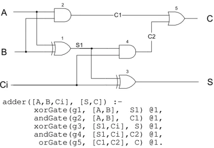
model is expressed in some connectivity language specifying the I/O lines and signals of the system and its components. This is the case with the ISCAS’85 benchmark suite [ISCAS 1985, Brglez and Fujiwara 1985], the well known and most used set of benchmark circuits in the area. It comprehends a total of 11 combinational circuits (c17, c432, c499, c880, c1355, c1908, c2670, c3540, c5315, c6288 and c7552), where the number in a circuit name indicates the number of signal lines (nets) in the circuit. The simplest of them, c17, is described below as an example, and corresponds to the schematic diagram of Figure 2.9:
INPUT(1gat) INPUT(2gat) INPUT(3gat) INPUT(6gat) INPUT(7gat) OUTPUT(22gat) OUTPUT(23gat)
10gat = nand(1gat, 3gat) 11gat = nand(3gat, 6gat) 16gat = nand(2gat, 11gat) 19gat = nand(11gat, 7gat) 22gat = nand(10gat, 16gat) 23gat = nand(16gat, 19gat)
Primary inputs and primary outputs are explicitly stated. The definition of gates follows the form output = type(input_list) which specifies the gate type (whose functional model is assumed to be known) and its I/O terminals (a single output and functionally equivalent inputs). Signal names in these terminals implicitly describe interconnections. For instance, primary input 3gat is connected to nand-gates 10gat and 11gat.
1gat
2gat
3gat 6gat
7gat
10gat
11gat
16gat
19gat
22gat
23gat
Figure 2.9. c17 ISCAS’85 example circuit
Figure 2.10. Graph representation of c17
It is easy to verify that c17 presents reconvergent fanout, with (for instance) two paths from 11gat (11gat 16gat 23gat and 11gat 19gat 23gat) reconverging at node 23gat.
Remembering the definitions of transitive fanin and fanout we see that, for example, the transitive fanout of 11gat is {16gat, 19gat, 22gat, 23gat} and the transitive fanin of 22gat is {1gat, 2gat, 3gat, 6gat, 10gat, 11gat, 16gat}.
Table 2.2 shows some statistics concerning each benchmark, including the number of PIs, POs, gates, circuit level, and average and maximum fanin and fanout, where a gate fanin is the number of its inputs.
circuit PI PO gates level
avg fanin
max fanin
fanout stems
fanout lines
avg fanout
max fanout
c17 5 2 6 3 2.00 2 3 6 1.27 2
c432 36 7 160 17 2.10 9 89 236 1.75 9
c499 41 32 202 11 2.02 5 59 256 1.81 12
c880 60 26 383 24 1.90 4 125 437 1.70 8
c1355 41 32 546 24 1.95 5 259 768 1.87 12
c1908 33 25 880 40 1.70 8 385 995 1.67 16
c2670 233 140 1193 32 1.74 5 454 1244 1.55 11
c3540 50 22 1669 47 1.76 8 579 1821 1.72 16
c5315 178 123 2307 49 1.90 9 806 2830 1.81 15
c6288 32 32 2416 124 1.99 2 1456 3840 1.97 16
c7552 207 108 3512 43 1.75 5 1300 3833 1.68 15
Table 2.2. Lines’ statistics of ISCAS benchmarks
Circuit buffer not and nand or nor xor Total
c17 6 6
c432 40 4 79 19 18 160
c499 40 56 2 104 202
c880 26 63 117 87 29 61 383
c1355 32 40 56 416 2 546
c1908 162 277 63 377 1 880
c2670 196 321 333 254 77 12 1193
c3540 223 490 498 298 92 68 1669
c5315 313 581 718 454 214 27 2307
c6288 32 256 2128 2416
c7552 534 876 776 1028 244 54 3512
Table 2.3. Gates' statistics of ISCAS benchmarks
For test generation problems, the ISCAS benchmarks include a set of single stuck-at faults (SSF) for each circuit (Table 2.4). Benchmark faults are only a subset of all the possible faults in a circuit (which are twice the number of nets, since any net may be stuck-at-0 or stuck-at-1), in fact, they constitute a collapsed fault set [Brglez and Fujiwara 1985]. The complete set of possible SSFs is collapsed to a smaller set since faults that are functionally equivalent to some other may be discarded. Two faults f and g are said to be functionally equivalent if the circuit presents always the same behaviour under the presence of fault f or g. For instance, an and-gate s-a-0 is functionally equivalent to any input i s-a-0 (as long as i has no fanout). In addition, the fault set may be further collapsed by considering the fault dominance relation [Abramovici et al. 1990]. Fault f dominates g iff any test that detects*g also detects f (on the same primary outputs), i.e. the set of tests that detect f contains g’s. As an example, for z = x and y, the single test that detects g = x s-a-1 is t = 01 that also detects f = z s-a-1. Fault f thus dominates g and can be discarded.
c17 c432 c499 c880 c1355 c1908 c2670 c3540 c5315 c6288 c7552 Faults 22 524 758 942 1574 1878 2746 3425 5350 7744 7550
Table 2.4. ISCAS circuits: Fault sets
2.5 Our Modelling Approach
We have adopted a structural gate-level code-based modelling for the ISCAS benchmarks. It is a gate-level model since the lowest-level primitive components are gates (including the xor-gate) that cannot be structurally decomposed. The logic value of each signal line is given by a different variable. Hence, to allow for different values in different fanout branches from the same stem (due to circuit faults), each branch is replaced by a buffer outputting a different variable. The same happens with PIs as Figure 2.11 illustrates with the c17 circuit. It is a code-based model because we have used a programming language (PROLOG [Lloyd 1988, Sterling and Shapiro 1994]), as well as its constraint logic programming extensions to more efficiently tackle different circuit problems.