Escola de Engenharia Departamento de Informática
Master’s Thesis
Master in Informatics Engineering
Science Data Vaults
in MonetDB: A Case Study
João Nuno Araújo Sá
Supervisors:
Prof. Dr. José Orlando Pereira
Departamento de Informatica, Universidade do Minho Prof. Dr. Martin Kersten
Centrum Wiskunde & Informatica, Amsterdam
Name:João Nuno Araújo Sá
Email:joao.nuno.a.sa@gmail.com
Telephone: +351964508853
ID Card:13171868
Thesis Title:Science Data Vaults in MonetDB: A case study
Supervisors:
Prof. Dr. José Orlando Pereira Prof. Dr. Martin Kersten Dra. Milena Ivanova
Year of Completion:2011
Designation of Master: Master in Informatics Engineering
É AUTORIZADA A REPRODUÇÃO INTEGRAL DESTA TESE APENAS PARA EFEITOS DE INVESTIGAÇÃO, MEDIANTE DECLARAÇÃO ESCRITA DO INTERESSADO, QUE A TAL SE COMPROMETE.
University of Minho, 13th July 2011 João Nuno Araújo Sá
Experience is what you get when you didn’t get what you wanted. Randy Pausch (The Last Lecture)
Acknowledgments
To Dr. José Orlando Pereira for accepting being my supervisor and for giving me this possibility to do my master thesis in Amsterdam. Apart from the distance, all the emails and recommendations were very helpful and I am thankful.
To Dr. Martin Kersten for receiving me in such a recognizable place as CWI and providing me the opportunity to be responsible for this project.
To Bart Scheers for all the patience talking about astronomical concepts and suggest-ing ideas to build a robust and solid use case.
A special thanks to Milena Ivanova for all the support, advice, inspiration and friend-ship. During all the meetings her help was essential, and to all the intensive corrections on the text I am extremely grateful.
To all the people of CWI, in particular the INS-1 group, for making me feel one of them through their sympathy and professionalism.
Ao meu pai, José Manuel Araújo Fernandes Sá e à minha mãe, Fernanda da Conceição Pereira de Araújo Sá, por todo o apoio, compreensão e saudades durante este ano que estive fora.
A toda a minha família, aos meus velhos amigos de Viana do Castelo e aos amigos que fiz em Braga.
To all my Amsterdam friends for making this year memorable. I will never forget the moments we had together.
Resumo
Hoje em dia, a quantidade de dados gerada por instrumentos científicos (dados cap-turados) e por simulações de computador (dados gerados) é muito grande. A quantidade de dados está a tornar-se cada vez maior, quer por melhorias na precisão dos novos intru-mentos, quer pelo aumento do número de estações que recolhem os dados. Isto requere novos métodos científicos que permitam analisar e organizar os dados.
No entanto, não é fácil lidar com estes dados, e com todos os passos pelos quais ne-cessitam de passar (capturar, organizar, analisar, visualizar e publicar). Muitos são colec-cionados (captura), mas não são selecolec-cionados (organização, análise) ou publicados.
Nesta tese focamo-nos nos dados astronómicos, que são geralmente armazenados em ficheiros FITS (Flexible Image Transport System). Vamos investigar o acesso a esses da-dos, e pesquisar informação neles contida, utilizando para isso uma tecnologia de base de dados. A base de dados alvo é o MonetDB, uma base de dados de armazenamento por colunas, de código livre, que já demonstrou ter sucesso em aplicações que analisam a carga de trabalho e aplicações científicas (SkyServer).
Perante os resultados obtidos durante as experiências, a perceptível superioridade apresentada pelo MonetDB em relação à ferramenta STILTS quando mais computação é exigida, e por último, pelo sucesso na execução do conjunto de testes apresentado pelo astronómo que trabalha no CWI, podemos afirmar que o MonetDB é uma alternativa forte e robusta para manipular e aceder informação contida em ficheiros FITS.
Abstract
Nowadays, the amount of data generated by scientific instruments (data captured) and computer simulations (data generated) is very large. The data volumes are getting bigger, due to the improved precision of the new instruments, or due to the increasing number of collecting stations. This requires new scientific methods to analyse and organize the data.
However, it is not so easy to deal with this data, and with all the steps that the data have to get through (capture, organize, analyze, visualize, and publish). A lot of data is collected (captured), but not curated (organized, analyzed) or published.
In this thesis we focus on the astronomical data, typically they are stored in FITS files (Flexible Image Transport System). We will investigate the access and querying of this data by means of database technology. The target database system is MonetDB, an open-source column-store database with record of successful application to analytical workloads and scientific applications (SkyServer).
Given the results of the experiments, the perceptible superiority presented by Mon-etDB over STILTS when more computation is required, and the success obtained during the execution of the use case proposed by an astronomer working at the CWI, we can declare that MonetDB is a powerfull and robust alternative to manipulate and access information contained in FITS files.
Contents
1 Introduction 1
1.1 The need to integrate with repositories . . . 2
1.2 Assumptions . . . 3 1.3 Contributions . . . 3 1.4 Approach . . . 4 1.5 Project Objectives . . . 4 1.6 Outline of report . . . 4 2 Background 7 2.1 Introduction to MonetDB . . . 7 2.2 Introduction to FITS . . . 8
2.2.1 Applications of the FITS . . . 9
2.2.2 The structure of a FITS file . . . 9
3 Contribution to MonetDB 13 3.1 Overview of the vaults . . . 13
3.2 Architecture of the vault . . . 14
3.3 Attach a file . . . 15
3.4 Attach all FITS files in the directory . . . 16
3.5 Attach all FITS files in the directory, using a pattern . . . 16
3.6 Table loading . . . 17
3.6.1 Search for the ideal batch size . . . 21
3.6.2 BAT size representation of Strings in MonetDB . . . 31
3.7 Export a table . . . 33 xi
4 Case Study 37
4.1 Overview . . . 37
4.2 Attach a file . . . 37
4.3 Attach all FITS files in the directory . . . 38
4.4 Attach all FITS files in the directory, giving a pattern . . . 38
4.5 Load a table . . . 38
4.6 Export a table . . . 39
4.7 Cross-matching astronomical surveys . . . 39
4.7.1 Query 1: Distribution of distances between sources in both surveys 41 4.7.2 Distribution of the distances smaller than 45 arc seconds . . . 44
4.7.3 Normal Distribution of all the data . . . 46
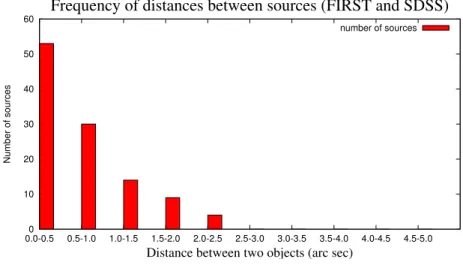
4.7.4 Frequency of the distances smaller than 5 arc seconds . . . 47
4.7.5 Frequency of the r value between sources in both surveys . . . 48
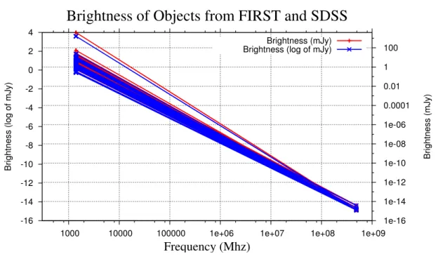
4.7.6 Query 2: extract & compare brightness in different frequencies . . 49
4.7.7 Query 3: extract the spectral index . . . 51
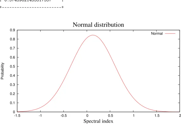
4.7.8 Distribution of the spectal index . . . 51
4.7.9 Normal distribution of the spectral indexes . . . 52
5 Performance Experiments 55 5.1 Experimental Setting . . . 55
5.2 Test Files . . . 56
5.3 Delegation experiments . . . 58
5.3.1 Selection and Filter delegation for Group number 1 . . . 58
5.3.2 Range Delegation for Group number 1 . . . 65
5.3.3 Statistics Delegation for Group number 1 . . . 69
5.3.4 Selection and Filter Delegation for Group number 2 . . . 71
5.3.5 Range delegation for Group number 2 . . . 73
5.3.6 MonetDB problem . . . 77
5.3.7 Projection delegation for Group number 2 . . . 80
5.3.8 Statistical Delegation for Group number 2 . . . 80
CONTENTS xiii
5.3.10 Equi-join delegation for Group number 3 . . . 83
5.3.11 Band-join delegation for Group number 3 . . . 88
6 Related Work 93 6.1 CFITSIO . . . 93 6.1.1 Fv . . . 96 6.2 STIL . . . 97 6.2.1 TOPCAT . . . 102 6.2.2 STILTS . . . 106
6.3 Comparison between tools . . . 107
6.4 Astronomical data formats . . . 107
6.4.1 HDF5 Array Database . . . 107
6.4.2 VOTable . . . 109
6.4.3 Comparison between file formats . . . 111
7 Conclusion 113 7.1 Results and Overview . . . 113
7.2 Future Work . . . 114
List of Figures
3.1 Three layers of a vault . . . 14
3.2 Load of all the numerical types . . . 19
3.3 BAT and File sizes for each one of the numerical types . . . 20
3.4 Batch 1 for the strings with 4 bytes . . . 22
3.5 Batch 1 for the strings with 8 bytes . . . 22
3.6 Batch 1 for the strings with 20 bytes . . . 22
3.7 Batch 10 for the strings with 4 bytes . . . 23
3.8 Batch 10 for the strings with 8 bytes . . . 24
3.9 Batch 10 for the strings with 20 bytes . . . 24
3.10 Batch 20 for the strings with 4 bytes . . . 25
3.11 Batch 20 for the strings with 8 bytes . . . 25
3.12 Batch 20 for the strings with 20 bytes . . . 26
3.13 Batch 50 for the strings with 4 bytes . . . 27
3.14 Batch 50 for the strings with 8 bytes . . . 27
3.15 Batch 50 for the strings with 20 bytes . . . 27
3.16 Batch 100 for the strings with 4 bytes . . . 28
3.17 Batch 100 for the strings with 8 bytes . . . 28
3.18 Batch 100 for the strings with 20 bytes . . . 28
3.19 Batch 1000 for the strings with 4 bytes . . . 29
3.20 Batch 1000 for the strings with 8 bytes . . . 29
3.21 Batch 1000 for the strings with 20 bytes . . . 30
3.22 Loading strings with 4 bytes . . . 30
3.23 Loading strings with 8 bytes . . . 30 xv
3.24 Loading strings with 20 bytes . . . 31
3.25 Representation of the space occupied by the strings with the size of 4 bytes 32 3.26 Representation of the space occupied by the strings with the size of 8 bytes 32 3.27 Representation of the space occupied by the strings with the size of 20 bytes 33 3.28 Export the numerical types into a FITS file . . . 35
3.29 Export the strings into a FITS file . . . 35
4.1 Distribution of distances between sources . . . 45
4.2 Normal Distribution . . . 47
4.3 Frequency of distances between sources that are less than 5 arc seconds apart from each other . . . 47
4.4 Measure of the brightness in different frequencies . . . 50
4.5 Calculation of the spectral index . . . 51
4.6 Plot of the Normal distribution of the spectral index . . . 53
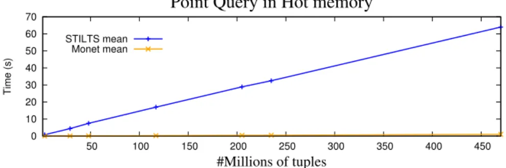
5.1 Performance of MonetDB and STILTS in Point Query operations with nu-merical types . . . 59
5.2 Performance of MonetDB and STILTS in Point Query operations for short type . . . 59
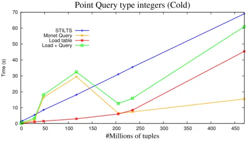
5.3 Performance of MonetDB and STILTS in Point Query operations for inte-ger type . . . 60
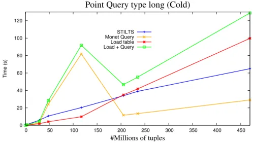
5.4 Performance of MonetDB and STILTS in Point Query operations for long type . . . 61
5.5 Performance of MonetDB and STILTS in Point Query operations for float type . . . 61
5.6 Performance of MonetDB and STILTS in Point Query operations for dou-ble type . . . 62
5.7 Performance of MonetDB and STILTS in Point Query operations with dif-ferent string sizes . . . 63
5.8 Performance of MonetDB and STILTS in Point Query operations with sin-gle 4-byte string column . . . 64
5.9 Performance of MonetDB and STILTS in Point Query operations with sin-gle 8-byte string column . . . 65
LIST OF FIGURES xvii 5.10 Performance of MonetDB and STILTS in Point Query operations with
sin-gle 20-byte string column . . . 65
5.11 Performance of MonetDB and STILTS in Range operations with numerical types . . . 67
5.12 Performance of MonetDB and STILTS in Range operations for short type . 67 5.13 Performance of MonetDB and STILTS in Range operations for integer type 67 5.14 Performance of MonetDB and STILTS in Range operations for long type . 68 5.15 Performance of MonetDB and STILTS in Range operations for float type . 68 5.16 Performance of MonetDB and STILTS in Range operations for double type 68 5.17 Performance of MonetDB and STILTS in statistical operations for short type 69 5.18 Performance of MonetDB and STILTS in statistical operations for short type 69 5.19 Performance of MonetDB and STILTS in statistical operations for integer type . . . 70
5.20 Performing of MonetDB and STILTS in statistical operations for long type 70 5.21 Performance of MonetDB and STILTS in statistical operations for float type 70 5.22 Performance of MonetDB and STILTS in statistical operations for double type . . . 71
5.23 Performance of Monet and STILTS in Point Query operations . . . 72
5.24 Performance of Monet and STILTS in Point Query operations . . . 72
5.25 Performance of Monet and STILTS in Point Query operations . . . 73
5.26 Performance of Monet and STILTS in Range operations . . . 74
5.27 Performance of Monet and STILTS in Range operations . . . 76
5.28 Problem on Monet with the table of 1G . . . 77
5.29 Performance of MonetDB and STILTS in Point Query Operations . . . 78
5.30 Performance of MonetDB and STILTS in Range Operations . . . 78
5.31 Performance of MonetDB and STILTS in Range Operations . . . 79
5.32 Performance of Monet and STILTS in Projection operations . . . 80
5.33 Performance of Monet and STILTS in Statistics operations . . . 81
5.34 Performance of Monet and STILTS in Statistics operations . . . 81
5.35 Performance for the different fan-out factors . . . 84
5.36 Percentage of memory consumed . . . 85
5.38 Percentage of memory consumed . . . 88 5.39 Performance for the different fan-out factors . . . 89 5.40 Percentage of memory consumed . . . 90
List of Tables
3.1 First group of FITS files . . . 18
5.1 Second group of FITS files . . . 57
5.2 Third group of FITS files . . . 57
6.1 List of operations performed by the tools . . . 107
6.2 Tasks performed for each one of the file formats . . . 111
Chapter 1
Introduction
In the past, scientific data was collected and stored predominantly in files. Using the file system is easy and practical but it has a number of disadvantages. First, files have no metadata, they do not benefit the evolution of data analysis tools, they do not have a high-level query language and the query methods will not do parallel, associative, temporal, or spatial search.
One strategy used by scientists to overcome the lack of metadata in files, is to provide extra information in the file name, allowing for the data of interest to be filtered efficiently. For example, the file name "January2010Hubble" describes that data was captured in January, 2010, by the space telescope named Hubble. The disadvantages of this approach are: limited number of parameters can be encoded in the file name, specific software needs to be written to understand the names, and we can have very long file names.
However, scientists prefer to use files instead of databases [17]. And when they are confronted about the reason why do not use databases, there is a huge range of answers they give:
• They do not benefit with the utilization of them • The cost of learning the tools is not worth it
• They do not have a good visualization/plotting of the results or because they use their own programming language
• Because there are incompatible scientific data types such as N-dimensional arrays and spatial text which are very difficult to support
• Because is to slow (loading takes too long, and sometimes it is not the data they need)
• Because once the scientific data is loaded, it cannot be manipulated anymore using standard applications.
In other words, database systems were not initially built to support science’s core data types. Therefore, a big evolution is needed before a second look by the scientists. How-ever, things are different now. The datasets are becoming bigger and bigger (peta-scale), file-ftp will not work with such a huge amount of data, and scientists need databases for their data analysis, for non-procedural query analysis, automatic parallelism, and search tools. Another way to access the data is needed. In the book "The 4th Paradigm" [17], Jim Gray describes those problems, emphasizing that better tools that support the whole re-search cycle need to be produced, from data capturing and data curation to data analysis and visualization. He also affirmed that the science evolution developed in the following four paradigms:
• It belongs to thousands of years ago, when science was only experimental and em-pirical.
• When it turned into theoretical science (some hundreds of years ago) with its equa-tions, laws and models.
• In the last few decades, the theoretical paradigms got so complex and complicated to solve analytically that some simulation was needed. With this, computational science was born, resulting in a huge amount of data generated by the simulations. • Data exploration, where the data is either captured by instruments or generated by simulations before being processed by software and finally stored in computers. The scientists only look at the data at the end of this whole process.
1.1
The need to integrate with repositories
It is essential to have good metadata, describing data in standard terms, so people and programs can understand it. In the scientific community, data must be correctly documented and must be published in a way that allows easy access and automated manipulation.
Predominately the reasons why we need to integrate with repositories are as follows. Firstly, they already have their own metadata. Secondly, they have their own way to structure the data. Thirdly, they were built with the purpose to supply answers to a specific community of scientists that already have their own unique demands. Database integration of the repository will extend functionality with the minimum investment.
1.2. ASSUMPTIONS 3
1.2
Assumptions
The first assumption of this work is that it is limited to a specific scientific community: astronomy, and to a particular format used in astronomy: FITS.
FITS is the standard astronomical data format endorsed by both NASA (National Aeronautics and Space Administration) and the IAU (International Astronomical Union). It also has the data structured in a standard scheme and it is extremely easy to get access to FITS files. They are available in thousands of websites: [6] and [5] are some examples of them. There are also some well known surveys that produce data using FITS files as output: FIRST [26], SDSS [4], and UKIDSS [7] for example.
The last assumption is that we limit ourselves to MonetDB, a powerful column-store database that is being developed in CWI, Amsterdam. It has the advantage of being open-source and built for analytical applications. The fact of being open source brings advantages. The availability of the source code and the right to modify it, enabling the unlimited tuning and improvement of a software product, as it is referenced in [15], is one of them. Applied to our case, allowed the creation of a new module and the development of new functionalities, inside MonetDB code.
1.3
Contributions
Our contributions to this project are a seamless integration of FITS vaults with Mon-etDB, through the development of a module inside the MonetDB code, that will provide a set of functionalities and it will provide a powerfull alternative to access and manipulate FITS files. We support only FITS Tables.
Once the FITS vault is understood, through the analysis of the metadata and the data model, it can be expressed in a relational database system.
The described alternative is based on a set of experimentations which are handled using MonetDB. It uses a fully new integration of FITS files with the database world that is ready to support an intricate set of astronomical questions that only databases can answer. The databases are enabled to process this data because they are developed and maintined for this purpose.
1.4
Approach
We do a bottom-up evaluation of the primitive needs that access and manipulate FITS files. The context is limited to FITS files, but we must keep others in mind. How could we work with other formats that are able to store astronomical data, how can we access their metadata and which properties do we have to understand in order to draw the data model in the relational database system. Another important factor that must be consid-ered is what are the differences between them and the FITS format. All this questions will be answered in the Related Work section, where we compare FITS files with others astronomical file formats.
1.5
Project Objectives
The main objective of this thesis is to study what extensions of a modern database architecture are needed, to provide the system with the ability to understand scientific data in external formats. Such ability will provide the users-scientists with:
• View over repository of data files in FITS standard format. Such a view presents metadata of the files and allows users to locate data of interest by posting queries against the metadata;
• Automatic attachment of files and data of interest. Using this feature the user can avoid manual loading of high volumes of data, which is time- and labour-consuming. The system automatically ships the data to the database. Furthermore, only pre-selected data of interest will be touched;
• Declarative SQL queries for analysis;
• Data Integration. The system allows for complex analysis that includes combining, comparing, correlating data from different FITS files and repositories (through SQL join queries, missing in FITS tools).
1.6
Outline of report
In Chapter 2 we will provide some knowledge on the background required to under-stand the thesis work. We will describe some important features of MonetDB and FITS files. In Chapter 3 we will present our contribution to MonetDB. More precisely, we de-scribe the FITS vault module that was developed and some important decisions made during the design & development process. In Chapter 4 we illustrate the functionality
1.6. OUTLINE OF REPORT 5 of the module by conducting an astronomy use case. In Chapter 5 we will conduct ex-periments, comparing the performance of MonetDB with the existing tools that operate with FITS files. In Chapter 6 we will enumerate some libraries that provide a set of func-tionalities to manipulate and access FITS files. We will list some programs that use those libraries and investigate what they can and cannot do with the respect to our use case. Fi-nally, in Chapter 7, we will talk about the results and a overview about the entire project. We will end with some suggestions for future work.
Chapter 2
Background
In this chapter we introduce the main concepts that underly our project. Here we will introduce the MonetDB system, focusing on the enhancements that it brings to the database world and the benefit for the astronomy community, as a database engine de-signed and prepared to answer routine astronomical queries. Thereafter, a presentation about the FITS files will be undertaken, exploring their history, their characteristics and how they are structured.
2.1
Introduction to MonetDB
MonetDB [2] is an open-source column-oriented database management system devel-oped, since 1993 at CWI, Amsterdam. The column-store idea was born as a depend-able solution to solve the main bottleneck faced by the majority of database systems: the main-memory access. Vertical fragmentation is identified as the solution for database data structures, which leads to optimal memory cache usage [11].
It is implemented by storing each column of a relational table in a separate binary table, called a Binary Association Table (BAT). A BAT is represented in memory as an array of fixed-size two-field records [OID,value], or Binary UNits (BUN). Their width is typically 8 bytes. MonetDB executes a relational algebra called the BAT Algebra that is programmed with the MonetDB Assembler Language (MAL). With a binary table for each column of the relational table, the query execution model is also different from main stream systems, having one operator at a time over entire columns. All these changes in the database architecture led to a creation of a brand new software stack, innovating all layers of the Database Management System.
The three layers that compose MonetDB software stack are: the query language parser, the set of optimizer modules and the back-end (MAL interpreter). The query language
parser it has an optimizer that reduces the amount of data produced by intermediates and exploits the catalogue on join-indices. The output is a logical plan expressed in MAL. The optimizer module takes decisions based on cost-based optimizers and runs algorithms. This module is crucial for the efficiency of the database. The MAL interpreter maintains properties over the objects accessed to gear the selection of subsequent algorithms. For example, a Select operator can benefit from sorted-ness.
This provides a simplification of the database kernel, an ability to fully materialize intermediate results, efficiency in the query processing speed and high performances when dealing with complex queries on sizable amounts of data.
This database system has already proved to be an asset for real-life astronomy appli-cations (SkyServer project) [19], with the goal to provide public access to the Sloan Digital Sky Survey warehouse for astronomers and the wider public. MonetDB, and the column store approach, demonstrate that they are promising for the scientific domain. We will use MonetDB to store the data imported from external file formats, and provide the data when requests are made.
The MonetDB code can be extended with new functionality. Functions need to be compiled and brought into the MAL level, so they can be used in the SQL level. This ex-tensibility is done through a create procedure [21] in the SQL level. This will enable the user to call the functions and have access to the functionalities provided by the module.
2.2
Introduction to FITS
It was in Holland and in the United States of America that the first high quality images of the radio sky were produced. The decade was 1970 and the pioneers were the West-erbork Synthesis Radio Telescope (WSRT) in WestWest-erbork, Holland, and the Very Large Array (VLA) in New Mexico, United States of America.
Their wish was to combine the data derived from both instruments. The main prob-lem was that the two groups were observing at different frequencies. As a consequence, it was complex to exchange information, either because the institutions had their own way to organize the data (internal storage format), or because there were considerable differences in the architecture of their machines, using a distinct internal representation for the same number, for instance.
Lacking a standard format for the transport of images, everytime when an astronomer needed to take data from an observatory to a home institution, some special software had to be created, in order to convert (restructure and perform bit manipulations) the data from the original machine, to the format that was being used by the home institution.
2.2. INTRODUCTION TO FITS 9 With all this setbacks, creating a single interchange format for transporting digital images between institutions, in order to avoid all this heavy process was needed. The idea was that each institution would need only two software packages: one that would translate the transfer format into the internal format, used by the institution and one that would transform the internal format into the transfer format. The Flexible Image Transport System (FITS) [13], was created with the intention to provide such a transfer format.
2.2.1 Applications of the FITS
The inaugural applications of FITS were the Exchange of radio astronomy images be-tween Westerbork and the VLA and the Exchange of optical image data among Kitt Peak, VLA and Westerbork. Afterwards, the use of FITS has expanded and it is now being ex-plored as a data structure in a diversity of NASA-supported projects:
• X-ray data from the Einstein High Energy Astrophysics Observatory (HEAO-2) • Compton Gamma Ray Observatory
• Roentgen Satellite (ROSAT)
• Ultraviolet and visible from the International Ultraviolet Explored (IUE) and the
Hubble Space Telescope
• Infrared data from the Infrared Astronomical Satellite (IRAS) and the Cosmic Back-ground Explorer (COBE)
It is being used as a standard for gound-based radio and optical observations, for organizations such as National Radio Astronomy Observatory (NRAO), National Optical Astronomy Observatories (NOAO) and European Southern Observatory (ESO)
2.2.2 The structure of a FITS file
A FITS file is composed by a sequence of Header Data Units (HDUs), that can be fol-lowed by a set of special records. Each HDU is composed by one header and the data that follows. The header is a sequence of 36 80- byte ASCII card images containing key-word = value statements. There are three special classes of keykey-words: required keykey-words, reserved keywords and the ones that are defined by the user. The data that follows (also called data records) is structured as the header specifies and it is binary data. The size of each logical record is 23040 bits, equivalent to 2880 bytes. Each HDU consists of one or more logical records. The last record of the header is filled with ASCII blanks so it can fill
the 23040-bit lenght. The first HDU of a FITS file is called Primary HDU. The HDUs that follow the Primary HDU are called extensions. When the FITS files contains one or more extensions, it is most likely that the Primary HDU does not contain any data. When the FITS file does not contain extensions it is called a Basic FITS, that is a file containing only the primary header followed by a single primary data array.
The Primary HDU is the first HDU of a FITS file. It is composed of one header (Pri-mary Header) and the data that follows. If the Pri(Pri-mary HDU is alone in the FITS file (there are no extensions), so it will be called Basic FITS. It is not normal (except for FITS images) that a Primary HDU contains any data, but if it does, it has to be a matrix of data values, in binary format that it is called Primary Array.
The Extensions have the same overall organization of all the HDUs (one header and the data that follows) and they come after the Primary HDU, respecting the structure of the FITS file. The extensions brought some new functionalities to the FITS files:
• Transfer new types of data structures: Images, ASCII Tables and Binary Tables • Transfer collections of related data structures
• The data to be transported do not always fit conveniently into an array format • Transport of auxiliary Information
The Tables are used to store astronomical data that is collected and they contain rows and columns of data. In the FITS files there are two types of tables: the ASCII Tables and the Binary Tables. As the name says, the ASCII tables store the data values in an ASCII representation. The data appear as a character array, in which the rows represent the lines of a table and the columns represent the characters that make up the tabulated items. Each member of the array is one character or digit. Each character string or ASCII representation of a number are in the FORTRAN-77 format. As for the binary tables, they store the data in a binary representation. The binary tables are more efficient, compact (about half of the size for the same information content), support more features and the time spent converting to ASCII tables is eliminated. The display is not as direct as for ASCII tables. The data types that can be stored in the FITS tables are:
• L: Logical value: 1 byte • B: Unsigned byte: 1 byte • I: 16-bit integer: 2 bytes • J: 32-bit integer: 4 bytes
2.2. INTRODUCTION TO FITS 11 • K: 64-bit integer: 8 bytes
• A: Character: 1 byte
• E: Single precision floating point: 4 bytes • D: Double precision floating point: 8 bytes • C: Single precision complex: 8 bytes • M: Double precision complex: 16 bytes • P: Array Descriptor (32-bit): 8 bytes • Q: Array Descriptor (64-bit): 16 bytes
Chapter 3
Contribution to MonetDB
In this chaper we present our contribution to MonetDB, through the development of a vault module that provides a set of functionalities concerning to FITS files. We will do a short overview of the vault concept. Further, we will describe the architecture of a vault. Finally, we will list a set of procedures and functions that were developed to make the integration between FITS files and MonetDB possible.
3.1
Overview of the vaults
A vault can be defined as a safety deposit box or as a repository for valuable infor-mation. By conducting an analogy to computer science terms, a data vault can be seen as a folder that contain only images. Inside the same data vault, the objects have one important factor in common: the metadata. It is the metadata that they have in common that allows a possible distinction between different kinds of vaults, and even the ability to create a completely new data vault based on similar parameters of the objects.
What distinguishes the objects in the same vault is the data that they carry. For ex-ample, if the object is an image, we know that it will have pixels, height and width. However, the values that are assigned to each one of the attributes differ for each image. Knowing that, we can create a vault based on a directory of files. We just need to un-derstand their metadata (using appropriate tools that allow us to access it), what meta-data they have in common and what is their meta-data model. Comprehending the meta-data model, we can decide how it will be represented in the relational database system.
We will apply the term vault to our case study. Creating a vault directory of FITS files, that share the same metadata but for which each one contains its own information.
The system needs to understand the external formats that contain the scientific data 13
(FITS). Once this is understood, there will be a distinction between loading data and attaching data. The idea of loading high volumes of data will be abandoned as it is time consuming, and for the most part, it is not what the scientist requires. This concept allows for the attachment of data (automatic attachment of files to the database), providing the metadata to the scientists, giving them the opportunity to decide what is relevant. It will be a selective load, and it will take less time.
3.2
Architecture of the vault
Figure 3.1: Three layers of a vault
In Figure 3.1 we can identify three distinct layers: the metadata wrapper, the data wrapper and the functionality wrapper. The metadata wrapper reads and understands the metadata of the vault and decides how the data model can be efficiently represented in a relational database system. Looking to our FITS vault example, there are three func-tionalities that support this demand: Attach a file, Attach all the files in the directory and Attach all the files in the directory, giving a pattern.
The data wrapper loads a fragment of data of interest that was explicitly required into the database. Once again, analyzing our FITS vault case, there are two procedures that support this requirement: Load a table and Export a table. This will avoid loading huge amounts of data at once, restricting the load to small portions that might be of interest to the user. Once inside the database, the data can be queried, manipulated or even exported as a completely new FITS file.
syn-3.3. ATTACH A FILE 15 chronization when the repository is updated. For the load on demand procedure, the idea is to enable the user with the ability of typing a query to the system and the func-tionality wapper will decide which FITS files will be attached and which tables will be loaded, in order to give the right answer to the user.
In the following sections we will describe each one of the functionalities listed before. All of them were implemented by building a module inside MonetDB code, that accesses FITS files and the FITS catalogue, through a library called CFITSIO [16]. The CFITSIO li-brary is written in C and provides a poweful interface for accessing, reading and writting FITS files. However, before using this library the user must have a general knowledge about the structured of a FITS file.
All the requests to the CFITSIO library are made using the C language. If the request demands some data filtering on the tables, a SQL query needs to be translated into MAL statements within MonetDB for execution.
3.3
Attach a file
We start with the attachment procedure, that opens a FITS file given its absolute name. After checking if the file has the FITS format, it scans the metadata that is present in its HDU and inserts descriptions of the table extensions to an internal FITS catalog. The catalog is composed out of the following tables:
fits_files
id: Primary key. Unique number that identifies the file name: absolute path to the attached file
fits_tables
id: Primary key. Unique number that identifies the table
name: name of the table that coincides with the name of the HDU. If the name is already taken by another table, it creates a new name, concatenating the name of the file, underscore and the number of the HDU which corresponds to the respective table
columns: number of columns present in the table
file: id of the file, that can be identified in the table fits_files
hdu: number of the HDU that the table represents in the FITS file (the number 1 is always reserved for the primary HDU)
date: this information is not always present in the FITS file. However, it stores the date when the FITS file was created
origin: similar to the date column, is data that is not always present. It stores the information about the station responsible for the creation of the FITS file
comment: sometimes FITS files have a field reserved for some additional infor-mation or comments that might be appropriate to supply.
fits_columns
id: Primary key. Unique number that identifies the column name: name that was given to the column within the table
type: the type of column represented in a FITS format. For instance: 8A repre-sents a string with 8 characters.
units: extra information about the units of the stored data: meters, kilometers, etc.
number: number of the column within the table
table_id: id of the table which the column is present. It can be identified in the table fits_tables
fits_table_properties
gives extra information about a table, such as extension, bitpix, stilvers (version of the product generating the file) and stilclas
3.4
Attach all FITS files in the directory
This procedure enables the attachment of all FITS files that are present in a specific directory, that is explicitly given as a parameter. If the directory can not be opened, a proper error message will be transmitted to the user. This pattern is useful because it avoids the attachment of the FITS files whithin a directory one by one, that is time consuming and exhaustive if the directory has thousands of FITS files.
3.5
Attach all FITS files in the directory, using a pattern
This procedure is an extension of the previous one. It adds the possibility of giving a pattern, in conjunction with the name of the directory, in order to diminish and limit the number of FITS files that are attached to the database. It works similar by the ls program used by UNIX. The advantage of this pattern follows the same idea as the previous one.
3.6. TABLE LOADING 17 However, it adds the option to give a pattern that will filter the FITS files attached. For example, suppose that there is a directory that has two thousand files, from which we are only interested in one thousand of them. If it is possible to build a pattern that will attach only those files of interest, we should call this procedure.
3.6
Table loading
Another feature designed was the load procedure, that loads the table with a given name. It searches the name in the FITS catalog, opens the corresponding file, moves to the matching HDU, creates an SQL table and loads the data into it. If the table is not described in the catalog, or it is already loaded, an appropriate error message will be returned. It calls a function from the CFITSIO library called fits_read_col. This function reads a column of the table and the data read are moved into an internal binary structure of MonetDB. This function will be called the same number of times as the number of columns present in the table.
This is an important and mandatory functionality, because it brings the data into the database system so it can be queried, processed and manipulated. The data type that takes more time to be loaded into MonetDB is the string type, due its unique structure in the database architecture. But more details on that will be studied in the upcoming chapters. This feature is in fact a bottleneck, when compared to existing tools that already query, process and manipulate data present in files. To make it work in the database world, the data needs to be first loaded from the files, so later it can give some answers to the users.
A fast mechanism to load the data into the database is essential. With this, it would be possible for a transition from the old and slow software tools world, to the more powerful and faster database system world.
In the further sections we will analyze the loading of different types of data into Mon-etDB. We will focus on one type at a time, building a set of FITS files, with only one column, that will contain the target type.
Each FITS file has only two HDUs: the Primary HDU, that is mandatory in each FITS file; and one extension, that contains a binary table with the type that we want to study.
With this group of tests, we can have a clear and succinct idea about how each one of the different types behaves. We will start with the column types that can be used to represent numbers.
• Short: any number between 0 and 32767 that occupies 2 bytes in MonetDB repre-sentation
• Integer: any number between 0 and 15000000 that occupies 4 bytes in MonetDB representation
• Long: any number between 0 and 2147483647 that occupies 8 bytes in MonetDB representation
• Float: any floating point number between 0 and 5 that occupies 4 bytes in MonetDB representation
• Double: any floating point number between 0 and 5 that occupies 8 bytes in Mon-etDB representation
Finally the column type String. Three different sets of FITS files will be created for this type: files that contain strings with the size of 4 bytes, files that contain strings with the size of 8 bytes and files that contain strings with the size of 20 bytes. The idea is to apply distinct benchmarks, with the same implementation, to the strings with different sizes.
Knowing the different types that will be studied, it is now time to enumerate the number of rows that each set of FITS files will contain:
FITS File Number of Rows
1 30000 2 2942000 3 29420000 4 58840000 5 117680000 6 205940000 7 235360000 8 470720000
Table 3.1: First group of FITS files
During the experiments, it was verified that the strings were the ones that took more time to be loaded into MonetDB and the type Short was the fastest, as we will see in the further tests. The measurements were done using GDKms() calls, in the FITS load routine, to measure the times it takes per column.
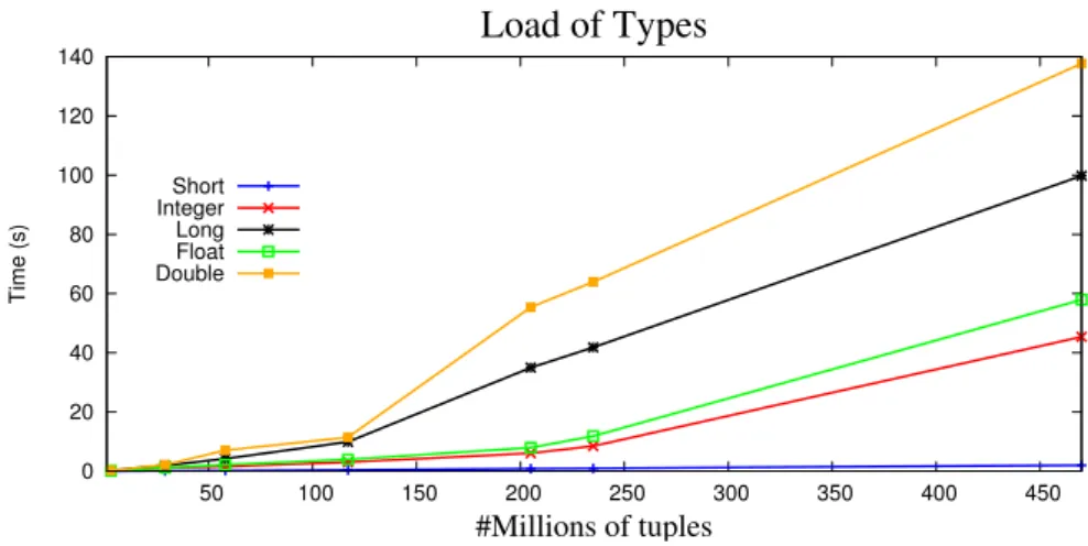
3.6. TABLE LOADING 19 0 20 40 60 80 100 120 140 50 100 150 200 250 300 350 400 450 Time (s) #Millions of tuples Load of Types Short Integer Long Float Double
Figure 3.2: Load of all the numerical types
Figure 3.2shows the time that took to load each one of the types in each one of the files. It can be noticed that the short type is the fastest and the double is the slowest. The type short is the fastest because it has the size of 2 bytes in MonetDB representation. There is a similarity between the loading time behavior of the integers and the loading time of the floats. This happens because both use 4 bytes in their MonetDB internal representation. Nevertheless, floating points are more complex to store, leading to a worse performance in the loading of the tables, when compared to integers. The same scenario takes place for the doubles and the longs. Both have 8 bytes in their MonetDB internal representation and both have a similar behavior in their loading time process, however, the double type is used to store floating point values. Consequently, there is a little additional time due to their complexity.
In order to understand some future behaviors, and taking advantage of the fact that the numerical types are already loaded into MonetDB, we can consult their BAT sizes in MonetDB internal representation and also the sizes of the original FITS files, where the data were in first place.
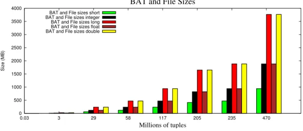
0 500 1000 1500 2000 2500 3000 3500 4000 0.03 3 29 58 117 205 235 470 Size (MB) Millions of tuples
BAT and File Sizes
BAT and File sizes short BAT and File sizes integer BAT and File sizes long BAT and File sizes float BAT and File sizes double
Figure 3.3: BAT and File sizes for each one of the numerical types
Figure 3.3represents the BAT and file sizes of each one of the numerical types. We realized that the BAT sizes in the internal representation of MonetDB are the same as the sizes of the FITS files that contain the original data, for all the types tested. So, instead of having two bars, representing the BAT size and the file size, for each one of the types, we draw only one bar, that represents both BAT and file size.
These results can be explained as follows:
• the short type takes 2 bytes in its representation. Multiplying 2 bytes for 470 mil-lions of tuples (the last file of the test) we get 940 MB, that is precisely the size of the last file that belongs to the set of files tested to the short type.
• the integer and float types use 4 bytes in their representation. As a consequence, the sizes of the BATs and the sizes of the files increase to the double (1.8 GB in the last file), comparing to the type short type.
• the types long and double occupy 8 bytes, that is twice the size of integers and floats. Fact that can be easily realized if we check the last BAT and file size of the respective types: (3.7 GB).
The next tests evaluate the loading of strings. We separate strings from numerical types due to the fact that strings are stored in a different way in MonetDB. In their internal representation, strings are composed by two different arrays:
• Tail: that contains pointers to the strings (it starts with a 4-byte size pointer) • Heap: that contains the actual strings
3.6. TABLE LOADING 21 During the experiments we found out that the string type needs longest time to be loaded. This statement can be proven by checking the loading times of the strings in the following set of graphs, comparing to the results of any other numerical type represented in Figure 3.2. Even for the string with 4 bytes, the loading time is worse than the loading time of the doubles, that are represented with 8 bytes.
To load the numerical and string types from the FITS files into MonetDB internal structure, two distinct processes need to be done:
• the call of the FITS library;
• the creation of MonetDB temporary BAT (appending time).
In order to improve the time to load the strings, several alternatives were imple-mented. The first alternative creates a big array with all the strings, the second performs a single call per string and the third is a middle term between the first and second ap-proach, reading a vector of strings at a time with a given size, and then load the data. The best alternative is the third, because it avoids the first case, where a lot of memory is being used and thus swapping to disk and it also prevents so many calls of the fits load function, that occurs in the second approach, which leads to a big overhead. For exam-ple, for a vector with the size 20, 19 fits load calls are avoided comparing to the second approach.
The following tests aim to find the optimal size of the batch, measuring the time that it takes to load the strings. Those measurements involve three different components:
• FITS library function calls;
• Append to MonetDB BAT structure; • Total time to load the strings.
We did not do this tests for the numerical types because the idea here is to optimize the time needed to load the slowest type, the strings.
50 100 150 200 250 300 50 100 150 200 250 300 350 400 450 Time (s) #Millions of tuples
Load of Strings (4 bytes) with batch size of 1
Load Append Sum
Figure 3.4: Batch 1 for the strings with 4 bytes
50 100 150 200 250 300 350 50 100 150 200 250 300 350 400 450 Time (s) #Millions of tuples
Load of Strings (8 bytes) with batch size of 1
Load Append Sum
Figure 3.5: Batch 1 for the strings with 8 bytes
50 100 150 200 250 300 350 400 450 50 100 150 200 250 300 350 400 450 Time (s) #Millions of tuples
Load of Strings (20 bytes) with batch size of 1
Load Append Sum
3.6. TABLE LOADING 23 We start with the batch size of 1, represented in Figure 3.4, Figure 3.5 and Figure 3.6. They are in fact the second approach that was mentioned before, performing a single call, to the fits library, per string. It can be noticed that loading the data, due to the fits library calls, takes always more time than the actual loading into the MonetDB data structure. For example, in Figure 3.4, for the last file, with 470 millions of tuples, the loading time is 143.3 seconds and the appending time is 111.2 seconds. The total time to load the strings into MonetDB is given as 323.1 seconds, meaning that a lot more computation is done in the background. As a final remark, the total time needed to load the strings with 4 bytes in the file with 417 millions of tuples is 323.1 seconds, to load the strings with 8 bytes is 371.4 seconds and to load the strings with 20 bytes is 458.3 seconds. The time needed to load through the fits library the strings with 4 bytes in the file with 417 millions of tuples is 143.3 seconds, to load the strings with 8 bytes is 163.9 seconds, and to load the strings with 20 bytes is 220.7 seconds. And finally, the time needed to load into MonetDB the strings with 4 bytes in the file with 417 millions of tuples is 111.2 seconds, to load the strings with 20 bytes is 138.8 seconds and to load the strings with 20 bytes is 168.4 seconds. We can easily perceive that the times are increasing while we augment the number of bytes that represent the strings.
20 40 60 80 100 120 140 160 50 100 150 200 250 300 350 400 450 Time (s) #Millions of tuples
Load of Strings (4 bytes) with batch size of 10
Load Append Sum
50 100 150 200 50 100 150 200 250 300 350 400 450 Time (s) #Millions of tuples
Load of Strings (8 bytes) with batch size of 10
Load Append Sum
Figure 3.8: Batch 10 for the strings with 8 bytes
50 100 150 200 250 300 50 100 150 200 250 300 350 400 450 Time (s) #Millions of tuples
Load of Strings (20 bytes) with batch size of 10
Load Append Sum
Figure 3.9: Batch 10 for the strings with 20 bytes
For the tests with batch size of 10, represented in Figure 3.7, Figure 3.8 and Figure
3.9 we got better results. This approach is in fact the first using the third alternative mentioned before, reading a vector of 10 strings at a time. The times are, in fact, faster than the tests performed in the Figure 3.4, Figure 3.5 and Figure 3.6, that use the batch size of 1.
In the last file, with 470 millions of tuples, the total time needed to load the strings with 4 bytes is 167.9 seconds. Much faster than the 323.1 seconds used in Figure 3.4. The responsible for this decrease in the time is the loading task, performed by the fits library. In the test with the batch size of 1 (Figure 3.4), it was 143.3 seconds and in the test with the batch size of 10 (Figure 3.7) it was 53.26 seconds. The appending time algo gets faster, being 111.2 seconds in Figure 3.4 and 107.7 seconds in Figure 3.7.
These are significant differences, and they are reflected in the other two tests, for the strings with 8 and 20 bytes (Figure 3.8 and Figure 3.9). Nevertheless, for this last two
3.6. TABLE LOADING 25 tests, an interesting fact occurs.
Note that in the transition from the file with 235 millions of tuples to the file with 470 millions of tuples, represented in Figure 3.8, the appending time starts to be faster than the loading time. This happens because MonetDB stops looking if there is a duplicate value in the dictionary of strings when the Heap size, that stores the strings, reaches the maximum size. The maximum size of the Heap corresponds to size of the main memory available in the system. When it reaches the maximum size, it just inserts at the end of the Heap. The insert of values it will be faster, as we can see in the graph, however it will be worse for the lookup operations, that will not be able to use the dictionary as a help.
As for Figure 3.9, the same happens, however, the Heap gets full earlier.
In this case in the transition from the file with 205 millions of tuples to the file with 235 millions of tuples. This happens because strings grew from 8 to 20 bytes, filling up the main memory faster.
20 40 60 80 100 120 140 50 100 150 200 250 300 350 400 450 Time (s) #Millions of tuples
Load of Strings (4 bytes) with batch size of 20
Load Append Sum
Figure 3.10: Batch 20 for the strings with 4 bytes
50 100 150 200 50 100 150 200 250 300 350 400 450 Time (s) #Millions of tuples
Load of Strings (8 bytes) with batch size of 20
Load Append Sum
50 100 150 200 250 300 50 100 150 200 250 300 350 400 450 Time (s) #Millions of tuples
Load of Strings (20 bytes) with batch size of 20
Load Append Sum
Figure 3.12: Batch 20 for the strings with 20 bytes
The tests with a vector of 20 strings read at a time are represented in Figure 3.10,
Figure 3.11and Figure 3.12. For the last file, with 470 millions of tuples, the total time needed to load the strings with 4 bytes is 148.2 seconds. It is an improvement, once the same test, for the batch size of 10, represented in Figure 3.7, needed 167.9 seconds. It is also an improvement for the strings with 8 bytes, represented in Figure 3.11. For the string with 20 bytes, there is a growth of 4 seconds comparing to the test with the batch size of 10, represented in Figure 3.9.
However, the intersection of the appending time with the loading time observed in
Figure 3.8does not occur in Figure 3.11. This happens because the loading time through the fits library gets faster with the batch size of 20 and the appending time into MonetDB has the same behavior. For example, with the batch size of 10, to load the strings of 8 bytes, in the last file with 470 millions of tuples, 114.9 seconds are needed. On the other hand, with the batch size of 20, the same test takes only 102.7 seconds. That difference is enough to avoid the intersection of times.
In Figure 3.12 the intersection happens again due the loading time, that gets once again slow, being exceeded by the appending time. Nevertheless, it is not enough to be considered a improvement compared to the same test with the batch size of 10, as we said before.
3.6. TABLE LOADING 27 20 40 60 80 100 120 140 50 100 150 200 250 300 350 400 450 Time (s) #Millions of tuples
Load of Strings (4 bytes) with batch size of 50
Load Append Sum
Figure 3.13: Batch 50 for the strings with 4 bytes
50 100 150 200 50 100 150 200 250 300 350 400 450 Time (s) #Millions of tuples
Load of Strings (8 bytes) with batch size of 50
Load Append Sum
Figure 3.14: Batch 50 for the strings with 8 bytes
50 100 150 200 250 300 50 100 150 200 250 300 350 400 450 Time (s) #Millions of tuples
Load of Strings (20 bytes) with batch size of 50
Load Append Sum
Figure 3.15: Batch 50 for the strings with 20 bytes
3.15, the results improved for all the string sizes. In conclusion, we can claim that this are the best results that we got till now.
20 40 60 80 100 120 140 160 50 100 150 200 250 300 350 400 450 Time (s) #Millions of tuples
Load of Strings (4 bytes) with batch size of 100
Load Append Sum
Figure 3.16: Batch 100 for the strings with 4 bytes
50 100 150 200 50 100 150 200 250 300 350 400 450 Time (s) #Millions of tuples
Load of Strings (8 bytes) with batch size of 100
Load Append Sum
Figure 3.17: Batch 100 for the strings with 8 bytes
50 100 150 200 250 300 50 100 150 200 250 300 350 400 450 Time (s) #Millions of tuples
Load of Strings (20 bytes) with batch size of 100
Load Append Sum
3.6. TABLE LOADING 29 For the vector size of 100, represented in Figure 3.16, Figure 3.17 and Figure 3.18, the results start to get worse because the size of the vector begins to be too large. With an average of 146 seconds, 218.5 seconds and 323.0 seconds to load the strings of 4, 8 and 20 bytes respectively, with the batch sizes of 20 and 50, as a total time to load the strings for the file with 470 millions of tuples, this tests with a batch size of 100 give us a total time of 165.9 seconds, 219.0 seconds and 324.4 seconds to load the strings of 4, 8 and 20 bytes respectively, in the last test with the file with 470 millions of tuples. As a consequence of this results, it is considered a bad result and it will not be selected.
20 40 60 80 100 120 140 160 50 100 150 200 250 300 350 400 450 Time (s) #Millions of tuples
Load of Strings (4 bytes) with batch size of 1000
Load Append Sum
Figure 3.19: Batch 1000 for the strings with 4 bytes
50 100 150 200 50 100 150 200 250 300 350 400 450 Time (s) #Millions of tuples
Load of Strings (8 bytes) with batch size of 1000
Load Append Sum
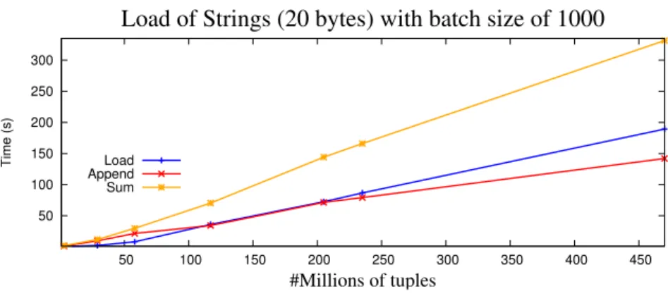
50 100 150 200 250 300 50 100 150 200 250 300 350 400 450 Time (s) #Millions of tuples
Load of Strings (20 bytes) with batch size of 1000
Load Append Sum
Figure 3.21: Batch 1000 for the strings with 20 bytes
For the last test, with a batch size of 1000, represented in Figure 3.19, Figure 3.20 and
Figure 3.21, there are no remarkable differences in the times, that make us look for bigger batch sizes, in order to find the perfect one.
0 20 40 60 80 100 120 140 160 0.03 3 29 58 117 205 235 470 Time (s) Millions of tuples
Overview of all batch sizes for string size of 4
Batch 10 Batch 20 Batch 50 Batch 100 Batch 1000
Figure 3.22: Loading strings with 4 bytes
0 50 100 150 200 0.03 3 29 58 117 205 235 470 Time (s) Millions of tuples
Overview of all batch sizes for string size of 8
Batch 10 Batch 20 Batch 50 Batch 100 Batch 1000
3.6. TABLE LOADING 31 0 50 100 150 200 250 300 0.03 3 29 58 117 205 235 470 Time (s) Millions of tuples
Overview of all batch sizes for string size of 20
Batch 10 Batch 20 Batch 50 Batch 100 Batch 1000
Figure 3.24: Loading strings with 20 bytes
With this experiments we were trying to find a close-to-optimal batch size. Figure
3.22, Figure 3.23 and Figure 3.24 show that the new approach of different batch sizes improved the loading times in all cases, but the best batch size seems different for diferent file sizes. In Figure 3.22, where the strings with 4 bytes were loaded, the batch size of 50 is slightly better than the other batch sizes. As for Figure 3.23 and Figure 3.24, there is no concrete answer about which batch size is actually better. They are all very close to each other and all of them describe the same behavior during the tests.
3.6.2 BAT size representation of Strings in MonetDB
As it was done for the numerical types, also a graph that represents the BAT size in the internal representation of MonetDB it will be done for the string type, with some addi-tional differences. In the following graphs, some addiaddi-tional information will be given:
• Tail size: Total size occupied by the string pointers • Heap size: Total size occupied by the strings
• Tail + Heap: Sum of the previous two sizes that represent the actual size used to store the string
• Memory: Line thats represents the total memory of the system • File size: the size of the FITS file where the data was originally
0 2000 4000 6000 8000 10000 12000 0 50 100 150 200 250 300 350 400 450 Size (MB) #Millions of tuples File with 4-byte Strings
Tail Heap Heap + Tail Memory File Size
Figure 3.25: Representation of the space occupied by the strings with the size of 4 bytes
Analysing the Figure 3.25, we can focus in five main occurrences. First, the linear growth on the FITS file size, obtained by multiplying the number of tuples times the 4 bytes of the string. Second, the transition in the Tail size, when it goes from the file with 235 millions of tuples to the file with 470 millions of tuples. This happens because the 4-bytes used as a pointer to the string are no longer enough. As a consequence, the size of the pointer needs to grow to 8 bytes. With the 8 bytes, there is space to represent all the pointers, however, the space needed to store them its bigger. Third, the Heap size also grows linearly, representing the size used to store the string. It needs 17 bytes to store each string of 4 bytes. Fourth, the memory line is exceeded, passing from the file with 235 millions of tuples to the file with 470 millions of tuples. This leads to future swapping operations, that will increase exponentially the time to execute some queries. The last and fifth fact that needs to be emphasized is the very high overhead of MonetDB for the short strings with 4 bytes: a FITS file with 2 GB takes 12G internally.
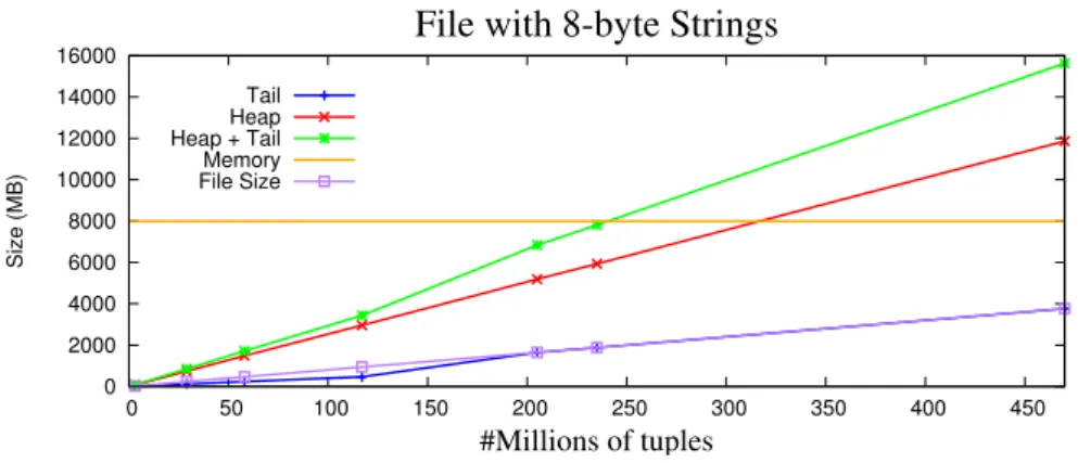
0 2000 4000 6000 8000 10000 12000 14000 16000 0 50 100 150 200 250 300 350 400 450 Size (MB) #Millions of tuples File with 8-byte Strings
Tail Heap Heap + Tail Memory File Size
3.7. EXPORT A TABLE 33 For the results presented in Figure 3.26, there is one occurrence that must be empha-sized, when compared to Figure 3.25. The transition in the Tail size that was observed in Figure 3.25, when going from the file with 235 millions of tuples to the file with 470 millions of tuples, this time happened in the file with 117 millions of tuples to the file with 205 millions of tuples. This happens because the strings have 8 bytes, instead of 4 bytes like in the previous test, consuming more heap space and also need to increase the address space for the pointers in the tail. As for the Heap size, it requires 25 bytes to store each string of 8 bytes. It uses 8 bytes more per string than in Figure 3.25.
0 2000 4000 6000 8000 10000 12000 14000 16000 18000 20000 0 50 100 150 200 250 300 350 400 450 Size (MB) #Millions of tuples File with 20-byte Strings
Tail Heap Heap + Tail Memory File Size
Figure 3.27: Representation of the space occupied by the strings with the size of 20 bytes In Figure 3.27, the transition in the Tail size occurs in the same interval, as the one observed in Figure 3.26, however, the bytes used to represent the strings are 20, that leads to a bigger space needed to store the strings. That fact is reflected in the sizes of the FITS files, that is bigger than the memory for the file with 470 millions of tuples. The same happen in the internal representation of MonetDB, that exceeds the memory size in the transition between the file with 117 millions of tuples and the file with 205 millions of tuples. As for the Heap size, it requires 34 bytes to store each string of 20 bytes. It uses 9 bytes more per string than in Figure 3.26.
3.7
Export a table
This procedure allows the user to create a completely new FITS file, based on an exist-ing table that is present inside the database. The file will have the name of the table, with the proper ".fits" extension. Once this function is called, the system will check if the table actually exists, giving a proper error message if not.
Assuming that the table exists, once the function is invoked, the properties of the table will be consulted: number of columns, types of the columns and number of tuples. This
information is used to create the header of the HDU containing the metadata about the table. With this information, we then need to collect the BATs that belong to each one of the columns in the table.
The optimal number of rows to write at once in the FITS file depends on the width of the table and the data types of the stored values. There is a routine in CFITSIO that will return the optimal number of rows to write for a given table, when given a FITS file as a parameter: fits_get_rowsize. We will use that routine to get the value. Each time the block of rows is full, the fits_write_col routine is called, and the rows that compose the block are added to the table present in the FITS file. This method of doing the export is much more efficient than calling the function only one time, which generates a big memory consumption. With this method we try to avoid the memory consumption problem, cleaning the block everytime that it is full and repopulating the array with the new data that needs to be added.
As we did before for the loading procedure, some measurements in the time needed to export each one of the types will be performed. We will start with the numerical types and finally we will export to a FITS file the three kinds of strings already studied before. The idea is to have a perspective about the types that take more time to be exported, so it can be manageable a proper future comparison with the existing tools that also provide the same functionality.
The time that will be checked is the one related with the invocation of the fits library function, fits_write_col.
The tables that will be exported are the same ones that were loaded into MonetDB in the loading section, with the same number of tuples and with only one column, that represents the target type that is being studied.
In Figure 3.28 we can realize that this strategy of writting the values with an optimal size, is in fact very efficient. The fastest type to be exported is the short type, due to the 2 bytes in MonetDB internal representation and the slowest is the double type, due to the 8 bytes in MonetDB internal representation. Another important point is the linear grow of the types till they reach the file with 235 millions of tuples. The growth behavior changes in the last file, with 470 millions of tuples, because it requires more memory and swapping operations, which leads to a worse result. As a last remark, the behaviour of the two groups: Integers, Floats and Longs, Doubles. Between them, they have the same behaviour till they reach the 235 million tuples file. For the file with 470 millions tuples, the types that require more computation and complexity (Floats and Doubles), need two or three additional seconds, than the numerical types that share the same number of bytes (Integers and Longs respectively).
3.7. EXPORT A TABLE 35 0 5 10 15 20 25 30 35 40 50 100 150 200 250 300 350 400 450 Time (s) #Millions of tuples Export of Numerical types
Short Integer Long Float Double
Figure 3.28: Export the numerical types into a FITS file
0 10 20 30 40 50 50 100 150 200 250 300 350 400 450 Time (s) #Millions of tuples
Export Strings with different sizes
Strings with 4 bytes Strings with 8 bytes Strings with 20 bytes
Figure 3.29: Export the strings into a FITS file
In Figure 3.29 we export the strings with 4, 8 and 20 bytes. For the strings with 4 bytes, the growth is linear till it reaches the file with 235 millions of tuples. After that, it grows faster because in MonetDB internal representation, for the file with 470 millions of tuples, the space needed to store the strings with 4 bytes exceeds the memory capacity, as we can see in Figure 3.25. As for the strings with 8 and 20 bytes, that change occurs earlier because to store this strings more space is required, as we can see in Figure 3.26 and Figure 3.27. Consequently, it will also take more time to export this strings.
Chapter 4
Case Study
In this section we will demonstrate, using a concrete example taken from astronomy, that the MonetDB-FITS combination works. That will be done through a step by step tutorial, guiding and explaning in detail to the astronomy user what needs to be done in order to get everything working and ready to be used.
4.1
Overview
We will present to the astronomer how can a specific FITS file be attached, accessing its metadata and spreading the information along several tables present in the SQL cat-alog. We will also exhibit how can the astronomer attach all the FITS files present in the directory, or even attach all the files present in the directory, giving a specific pattern. Further, we will explain how to load a specific table present in a FITS file that is already attached into the SQL catalog. Also how can we export a table present in our SQL catalog to a brand new FITS file. Finally, once all the astronomical data is present in the database we want to do something with it. As a suggestion proposed by an astronomer working at CWI, we will demonstrate how to execute a set of common astronomical queries in MonetDB. This will be the added value of this section, where we present MonetDB as a capable database engine that is ready to fulfil a set of astronomical demands.
We assume that the user already has MonetDB installed in the system, with its last version, downloaded from the Mercurial repository.
4.2
Attach a file
For this initial task, a FITS file must be present in the file system. Lets assume that the FITS file is called testattach.fit, and its directory is ’/ufs/fits/’. To attach the file into