Essays on monetary theory

(1)

D

OCTORAL

T

HESIS

Essays on Monetary Theory

Author:

Fernando Antônio de Barros Júnior

Supervisor: Ricardo de Oliveira Cavalcanti

A thesis submitted in fulfillment of the requirements for the degree of Doctor of Philosophy

Escola de Pós-Graduação em Economia

(2)

Barros Júnior, Fernando Antônio de

Essays on monetary theory / Fernando Antônio de Barros Júnior. – 2017. 102 f.

Tese (doutorado) - Fundação Getulio Vargas, Escola de Pós-Graduação em Economia.

Orientador: Ricardo de Oliveira Cavalcanti. Inclui bibliografia.

1. Política monetária. 2. Inflação. 3. Moeda. I. Cavalcanti, Ricardo de Oliveira. II. Fundação Getulio Vargas. Escola de Pós- Graduação em Economia. III. Título. CDD – 332.4

(3)

(4)

“... I kind of believe that some of the best economics consists of counterexamples. People think A is true, and someone builds a little model whose ingredients don’t seem particularly weird and it implies not A. And so you’ve got to confront that.”

(5)

Acknowledgements

First and foremost, I would like to thank God, whose many blessings have made me who I am today.

I am forever grateful to my advisor Ricardo de Oliveira Cavalcanti for his patience, guid-ance and support in my thesis. I am also indebted to Jefferson Donizeti Pereira Bertolai for his suggestions and help during the development of this thesis.

I would like to thank many colleges for comments and stimulating discussions. Specially Bruno Ricardo Delalibera, Valdemar Rodrigues de Pinho Neto, Rodrigo Bomfim Andrade and André Victor Doherty Luduvice. I have learned a lot from them and many other stu-dents at EPGE-FGV.

I also thank my girlfriend Regiane Paes, who has supported me throughout my academic trajectory, and my family.

Finally, I thankfully acknowledge financial support of Conselho Nacional de Desen-volvimento Científico e Tecnológico (CNPq), Fundação Carlos Chagas Filho de Amparo à Pesquisa do Estado do Rio de Janeiro (FAPERJ), Coordenação de Aperfeiçoamento de Pes-soal de Nível Superior (CAPES) and Graduate School of Economics at Fundação Getúlio Vargas (EPGE-FGV).

(6)

(7)

List of Figures

1.1 Salient features of pairwise trades. . . 26

2.1 Relative Optimum Welfare: core-off/core-on . . . 45

2.2 Distribution of money . . . 47

2.3 Optimal inflation . . . 48

2.4 Inflation varing the fraction of banks . . . 49

2.5 Distribution of money - monitoring. . . 50

3.1 Optimal allocation varying the discount factor . . . 63

3.2 Optimal allocation: selected output and price . . . 64

3.3 Optimal welfare . . . 66

3.4 Optimal allocation varying bond’s maturity . . . 67

(10)

(11)

List of Tables

1.1 Insurance when optimal inflation is zero: taxing consumers in meetings with

the poorest producer . . . 6

1.2 Savings according to profit rates . . . 13

1.3 Outside money, β = .9 and core on . . . 20

1.4 Outside money, β = .5 and core on . . . 21

1.5 Outside money, β = .9 and core off . . . 22

1.6 Outside money, β = .5 and core off . . . 23

1.7 Inside money and core off . . . 24

1.8 Inside money and core on . . . 25

1.9 Outside money in pairwise meetings: core on . . . 27

1.10 Outside money in pairwise meetings: core off. . . 28

2.1 Average Payment . . . 46

2.2 Selected Avarage Payment . . . 49

B.1 Pairwise meetings and core on . . . 76

B.2 Pairwise meetings and core off . . . 77

D.1 Deviatov and Wallace (2014) replication . . . 83

(12)

(13)

Introduction

In this thesis, we apply numerical methods to study some model where money is essen-tial. We follow the mechanism-design approach to monetary theory and search for settings where people can experience the higher welfare.

In chapter 1, we pursue more general simulations of the Shi-Trejos-Wright model with lump-sum transfers of fiat money, as well as develop a model of intermediation in tripar-tite meetings, to demonstrate the following implications of lack of commitment in match-ing models of money: savmatch-ings are inefficiently low; inflation has a negative effect on self-insurance; and although lump-sum transfers should be avoided in many specifications, pos-itive inflation can be optimal with inside money.

In chapter 2, we study the optimality of inflationary policies in a model of inside money. Our numerical findings indicates that inflation is optimal in matching models of money due to higher benefits of money creation than its effects on the return of money. This results holds for a board set of parameters, however, when people are patient and the fraction of monitored people is high enough, then inflation is not part of the optima.

In chapter 3, we introduce ‘open market operations’ in a matching model of money where inflationary policies are optimal - the social benefits of inflation are higher than its costs. Using the average utility as welfare criteria, we numerically solve the model for the best implementable allocation and find that having bonds in the economy can enhance so-cial welfare. In our model, bonds are immune to inflation, thus people value them more than money in equilibrium. Therefore, bond holders can consume more, but they also produce less than money holders. In steady state, both bonds and money circulate in the economy, which increases welfare due to a better distribution of consumption among people. In addi-tion, we present numerical examples to show maturity of bonds and monitoring affect the optimal allocation.

(14)

(15)

Chapter 1

A paradox of expansionary policies

1.1 Introduction

A recent consensus in monetary theory is that money is an imperfect mechanism.1 Absent interventions, it is a poor store of value. And the dynamics of monetary trades produces an uneven distribution of money, exposing traders to liquidity risks. The main lesson seems to be that a monetary program for creating liquidity can lessen these imperfections, hurting one dimension in order to improve the other.

A benchmark experiment involves models of pure currency, with people facing the risk of running out of money due to a particular sequence of trade opportunities. It is then asked whether lump-sum transfers of money improve welfare, relative to a zero-inflation equilibrium. Using variations of the Bewley (1980) model, Levine (1991) and Kehoe, Levine, and Woodford (1992) have tackled this question, thereby constructing an important coun-terexample to the Friedman (1953) and Friedman (1969) rule. Using particular assumptions, they focus, however, on Markov equilibria in which nominal payments are invariant to the inflation rate.

Keeping the distribution of money tractable and still capturing a negative effect of in-flation on output is certainly a step forward. In this paper, however, we argue that there is a key drawback in this forced simplification, because another negative effect of inflation is ignored. It is robust and can change the role of expansionary policies. Using matching models, we ask what happens when inflation is allowed to reduce savings. We then find a paradox: lump-sum transfers can actually make the risk-sharing problem worse when the distribution of money is sufficiently rich. Our point about monetary policy is that it should

(16)

be assessed by similar considerations related to crowding-out of self-insurance [see, for in-stance, the non-monetary model with private insurance markets and limited enforcement by Krueger and Perri (2011)].

Illustrating our point requires removing simplifications adopted by existing work, forc-ing us to appeal to numerical methods. Instead of a Bewley model, we use some variations of the basic random-matching model and provide a careful explanation why previous work has missed this paradox. Part is due to the misconception that main issue with inflation is the so called ‘hot potato effect’. One can indeed easily see in a cash-in-advance model that inflation reduces the return of money, producing a distortion as the real quantity of goods traded falls. But the ignored effect we are talking about is only present when the quantity of nominal savings is important, and this is not the case with a representative agent, or when the model allows for a quick rebalancing of money balances. In order to study the paradox, it is important to be able to exacerbate the role of nominal savings.2

The fact is that in matching models with fiat money, better incentives to save can prevent a negative externality from taking place: when sellers receive a high nominal payment they become less inclined to trade goods for money in the future, aside from the fact that each unit of money may have an inadequate return. In this paper, we illustrate this fact from dif-ferent but related angles. First, we explain why extensions of the models in Shi (1995) and Trejos and Wright (1995), pursued by Molico (2006) and Deviatov (2006), find a role for infla-tion: it is because the former does not allow for allocations that provide better insurance to poor money-holders, but which could introduce non-convexities, while the latter restricted the upper-bound on holdings in such a way that inflation was not reducing savings when expansionary policies mattered. Second, we find a way of making savings more important in a commodity-money version of Lagos and Wright (2005). In particular, we allow for tri-partite meetings, highlighting the importance of money holdings by intermediaries. Third, we revisit fiat-money exercises with this tripartite structure, discussing restrictions to ‘core’ allocations and the assumption that intermediaries can now be regulated. We then docu-ment the fact that, for many parameter specifications, savings are particularly low with core

2_{Bewley models (see recent application by Lippi, Ragni, and Trachter (}₂₀₁₄_{)) allow poor and rich traders}

to find a relatively fast regression to mean holdings because they participate in the same market every period. The speed of such redistribution, by contrast, is much slower in general matching models. This difference has not been emphasized in the literature (see Wallace,2014afor other novelties), but is key for understanding the paradox and may as well be present when inflationary transfers are used to pay interests on money (see Wallace,

(17)

allocations, but regulation of intermediaries can lessen the problem.

If Levine (1991) and Bewley (1980) are offering counterexamples to the Friedman rule, the reader may ask, to what previous research our results give more support? The related literature is a voluminous one. In the conclusion we make few remarks on the Wallace,

2014bconjecture that positive inflation in pure-currency economies should be optimal with

the possible exception of knife-edge specifications. In section 2 we mention some additional literature, while in section 6 we highlight passages of Bagehot (1873) as early references to the importance of keeping a proper distribution of money. Finally, section 7 concludes and the appendix contains proofs as well as auxiliary information about simulations.

1.2 A preview

Our counterexamples are selected from steady states, and focus on how traders can privately (self-) insure against shocks using currency, given that meetings are heterogeneous and ran-dom, while gains from trade can in principle be divided in a variety of ways, according to wealth profiles in each meeting.3 They also complement findings by Deviatov (2006), and Deviatov and Wallace (2014), about optimal policy with outside and inside money.4 Before describing novel ways to reinforce concerns with monetary savings (starting first with a quasi-linear model with commodity money, in the next session, and then with fiat money and more general preferences), we give now an overview of basic simulations to motivate that idea that even the simple pairwise-meetings model can give rise to robust counterex-amples.

3_{The idea that policy evaluation depends crucially on self-insurance and thus on available forms to store}

wealth motivates the empirical study of Krueger and Perri (2008). There is also a large literature featuring numerical work in Bewley models (such as Imrohoroglu (1992)). While in matching models (see an extensive survey by Lagos, Rocheteau, and Wright (2014)) negative effects of inflation on self-insurance have not been singled out, there is a remote relationship between our findings and the notion of constrained inefficiency (see Geanakoplos and Polemarchakis (1986)): an inefficiently high level of capital holdings in the Aiyagari (1994) model, for instance, generates an externality in the form of more labor-income risk (see Davila et al. (2012) and references therein). Finally, an empirical assessment of how redistributive effects of inflation depend on spend-ing possibilities, measured by the maturity structure of nominal assets, is the subject of Doepke and Schneider (2006).

4_{Instead of using a Bewley model, Cavalcanti and Nosal (}₂₀₀₉_{) propose another way of making flat}

ex-pansions appealing, using a simple matching model with just 0-1 holdings of money, and adding a seasonal pattern. In particular, they specify a utility jump for people specializing in consumption at a particular season and finding welfare gains when expansions target that season (see also Wallace,2014aand references therein). But negative effects of inflation in their setting are also narrowly defined (in their model policies are introduced to correct the problem that savings are too high in low seasons).

(18)

There are two key observations in these simulations. First, because consumption and production of a perishable good takes part in pairwise meetings, the social planner is not re-stricted to the ‘law of one price’ as in Bewley models. This means that allocations involving poor traders can be target so as to provide insurance with attractive ‘prices’ for this group, an alternative to inflationary policies affecting the whole population. Second, self-insurance in the form of money holdings depends on how wealth can be stored. In particular, in nu-merical simulations, if the upper bound on holdings is too small, expansionary policies gain an artificial edge over self-insurance.

Our simulations (presented in detail later) use lotteries, as in Berentsen, Molico, and Wright (2002), having the interpretation that people are spending (and receiving from the government, when expansionary policies are in effect) non-integer amounts of money. This approach is complemented by a proxy of inflation suggested by Li (1994) and Li (1995): the inflation tax is captured by some random confiscation of money holdings. As in many money models, these economies have people meeting randomly in pairs and trading per-ishable goods for fiat money as in Shi (1995) and Trejos and Wright (1995). Expected utilities associated with money holdings, v, must be consistent with payments and output produced in single-coincidence meetings. A social planner chooses from stationary allocations accord-ing to average utility. For an affordable numerical cost, we assume that money is indivisible and that goods are traded for lotteries on money holdings, with support {0, 1, 2, 3, 4}. There is a large set of possible stationary distributions of money and terms of trade: output and lotteries for each type of meeting, as indexed by traders’ wealth. Exchanges must be better than autarky in meetings for both traders and belong to the core (defined formally later). We have assembled, in Table 1, selected features of optimal allocations.

TABLE 1.1: Insurance when optimal inflation is zero: taxing consumers in meetings

with the poorest producer

β 0.9 0.8 0.7 0.6 0.5

i v/ tax v/ tax v/ tax v/ tax v/ tax

0 0.4514 / - 0.0263 / - 0.0089 / - 0.0018 / - 0.0013 / -1 1.2638 / 0.0000 0.5940 / 0.0000 0.3948 / 0.0000 0.2282 / 0.0000 0.2253 / 0.0000 2 1.5692 / 0.4067 0.7824 / 0.0000 0.5166 / 0.0000 0.3663 / 0.0502 0.2738 / 0.0698 3 1.7538 / 0.2271 0.8794 / 0.0000 0.5675 / 0.0000 0.3892 / 0.0000 0.2861 / 0.0000 4 1.9027 / 0.0552 0.9291 / 0.3964 0.5851 / 0.2921 0.4107 / 0.0000 0.3010 / 0.0000

Based on Table 9. v represents the expected discounted utility for each level of holdings i before meet-ings take place; In meetmeet-ings where the consumer holds i and the producer holds 0, ‘tax’ is computed as 1 − y/x, where y is actual output and x is the cuttoff level determining zero surplus for the producer, keeping fixed the optimal payment.

(19)

By letting a key parameter, the discount factor β, take different values, we allow the discrepancy between private and social objectives to vary: as we shall see later on, as β is increased, concerns about savings loses importance, so that there is more flexibility with respect to how taxation is levied. For now, some interesting insights are revealed by mea-sures of maximum output that poorest producers could be asked to hand out, given the expected utilities they are actually receiving as payments (not displayed). The relative dif-ferences between these ceilings and quantities actually delivered, labeled tax, represents a loss to consumers that varies with their holdings of money. According to Table 1, for all β, the poorest producer is always receiving a surplus in some meetings (identified by positive taxes). The precise wealth i of whom is taxed depends on β.

Now there are two remarks on previous work in connection with features of Table 1. First, in attempts to reproduce Levine,1991findings by Molico (2006) and Deviatov (2006), corresponding tax statistics are typically zero. In the former case, the tax is always zero due to a bargaining assumption. In the latter, as shown below, for examples with positive inflation the tax is zero because the support used was too small (a 2-unit upper bound), leading to a flatter v (less affected by Inada conditions). Second, we did allow for a lump-sum transfer of money followed by inflation in the same fashion as Deviatov,2006did, but no improvements were found. The reason, as mentioned above, is that inflation interacts adversely with self-insurance.

1.3 Adding more risk

We now describe how to make savings even more important in matching models. Adopting the mechanism-design perspective of Hu, Kennan, and Wallace (2009) and Cavalcanti and Puzzello, 2010, for the model of Lagos and Wright (2005), the idea is to require a form of intermediation in meetings, highlighting the importance of the distribution of money and, later, new effects when policies include regulation of inside money.

In this section, for simplicity, we avoid the discussion of interventions in the quantity of money. The goal for now is to show externalities in savings decisions. We model com-modity money in a version of quasi-linear economies due to Cavalcanti and Puzzello (2010). Random meetings are preceded by a subperiod in which people must decide how much to consume or to save in the form of a durable commodity. Ideally, society would have traders

(20)

choosing high savings at that moment. But since traders cannot commit there is an instance of the Jacklin (1987) problem: after people learn their types, and corresponding opportunity costs of carrying money holdings, they tend to choose lower levels of savings.5 It is then shown how consumption taxes can improve welfare relative to the alternative of giving all the surplus to consumers at the meetings stage.

In order to avoid complicated dynamic effects, we assume that commodity money is valued according to separable, linear utility. Relevant histories of savings are entirely cap-tured by recent preference shocks. When people trade in pairs taxation is not needed and consumers keep all gains from trade. But when intermediation is considered, and meetings include a third trader that can lend to consumers, we find that savings by intermediaries are important and that some interventions can provide a better allocation of risk.

1.3.1 A commodity-money environment

Time is discrete and each period is divided into two subperiods. The economy has a large population living forever and experiencing random meetings in the first subperiod, and preference shocks in the second. Preference shocks are realizations of an iid process. There is a durable good called money that can be consumed and produced in the second subpe-riod, according to an idiosyncratic marginal utility θ drawn every date from an uniform distribution. For simplicity, we assume a discrete support {θ1, ..., θn} and let F , such that

F (θi) = _ni for all i, denote the cumulative distribution of θ. In addition, we normalize its

mean, settingP

i 1 nθi= 1.

Money is hence a commodity, produced and consumed when people are by themselves, according to linear utility that is the realization of a preference shock. Money balances are planned in order to reach ideal savings, for each θ, for use as a medium of exchange in the next period, first subperiod, when random meetings take place. Money holdings are ob-servable in meetings but trade histories are private information and people cannot commit to future actions.

There is no discounting between first and second subperiods, but there is discounting at the common factor β across dates. We assume θiis increasing in i with θ1> β, so that savings

5_{In Jacklin (}₁₉₈₇_{), allowing traders to exchange claims on bank deposits eliminates risk sharing from deposit}

contracts. Hence trading after types are assigned allows people to avoid taxation. In monetary models, when a bank is not providing the final allocation of goods, it is necessary to discuss if trading is amplified by policy, in a version of the Lucas (1976) critique.

(21)

are always costly. There is also the standard specialization of production and consumption in meetings. We assume that every meeting is formed by three people: a producer, an in-termediary and a consumer. We assume that a person has equal probability of taking part in a meeting in any of these three occupations. And that the meeting is a single-coincidence meeting, when the first person can produce a perishable good for the third one, with proba-bility 3α, where α ≤ 1₃. With probability 1 − 3α there are no potential gains from trade. The utility of consuming c ∈ R+units of the perishable good is u(c), and the utility of producing

c units of the perishable good is −c. We assume that u(0) = 0 and that u is continuous, concave, differentiable and such that u0(0) = +∞and u(c) < c for c sufficiently large.

We assume that the only feasible trade in a meeting has the intermediary transferring money to the producer, as loan to the consumer, in exchange for goods produced. Then, after production takes place and the producer leaves the meeting, the consumer is able to receive goods and to pay out the loan with the intermediary.

In this economy, the planner’s problem is to maximize the present value of average utility by choice of incentive-compatible allocations that provide a suitable level of insur-ance against shock θ and exchange risk. Following Cavalcanti and Puzzello, 2010, we re-strict attention to stationary allocations. We also anticipate that, due to the quasi-linear structure, optimal allocations are not functions of past histories. A meeting is a vector m = (m1, m2, m3)describing holdings of money of the producer, m1, the intermediary, m2,

and the consumer, m3. An allocation is a list (s, x, y, z) describing saving plans s in the

sec-ond subperiod, as a function θ, and trade plans (x, y, z) in the first subperiod, as a function of m. Saving plans say how much money people will take with them when leaving the second subperiod, according to the realization of idiosyncratic shocks. Trade plans describe loan size x, output level y, and payment amount z. That is, z is the reduction in holdings of money suffered by the consumer, x is how much the producer receives, and z − x is the intermediation profit. We require money transfers to be feasible in the sense of x(m) ≤ m2

and z(m) ≤ m3.

A plan s : {θ1, ..., θn} → R+generates a distribution of money µ on R+. It is convenient

to denote by µ3 the distribution of meetings on R3+ generated by µ, and by µ2 it marginal

distribution on R2

(22)

the utility of an ex-ante representative agent and can be written as w(s, y) = − Z (θ − β)s(θ)dF (θ) + αβ Z (u(y(m)) − y(m))dµ3(m). (1.1)

Notice that the welfare function w does not depend on monetary payments. This is so be-cause expected utility, when leaving meetings, as a function of after-trade holdings, is the same for all traders. Hence, no matter how money is divided by trade, the average dis-counted value attached to after-trade holdings is βP

i n1s(θi).

1.3.2 Implementable allocations

We also follow the notion of implementability adopted by Cavalcanti and Puzzello, 2010, that is, that traders agree with (s, x, y, z), given µ associated to s, if autarky in meetings would not make them better off, and if there are no other saving choices that could improve individual utility given (x, y, z) and µ. We shall leave the discussion of group deviations for the fiat money environment of following sections. But while in Cavalcanti and Puzzello, 2010it is optimal to give all surplus to consumers, here this is not so due to an externality associated to savings decisions of people who end up in position to make loans.

In order to be implementable, an allocation must satisfy incentive constraints. Trade incentive constraints are given by

y(m) ≤ x(m), x(m) ≤ z(m) and z(m) ≤ u(y(m)). (1.2)

These inequalities ensure that trade surpluses are nonnegative in all meetings. The saving incentive constraint is that s(θ) must solve the problem of maximizing −(θ − β)k + αβv(k) by choice of money holdings k , where the expected gain from trade v(k) is defined by

v(k) =

Z

(u(y(a, a0, k)) − z(a, a0, k) + z(a, k, a0)

−x(a, k, a0) + x(k, a, a0) − y(k, a, a0))dµ2(a, a0). (1.3)

Because the distribution of money µ in turn must be generated by s, an incentive-compatible savings plan is a fixed point for each (x, y, z). Allocations that are feasible and incentive compatible are called implementable.

(23)

1.3.3 Welfare bounds

We are now ready to make two basic points about this intermediation economy. In this sub-section we show that there is essentially no friction leading to low savings if intermediation is either removed or if the distribution of shocks is degenerate. If constraints associated with intermediation are relaxed then we find no wedge between private incentives to save and the planner’s problem. In addition, the solution can be computed recursively: for a given distribution of savings, welfare is maximized by giving all trade surpluses to consumers; and given the implied rate of exchange between money and output, savings are chosen op-timally in a separable way according to the costs of supplying money (see proof of next proposition). In the next subsection, we show how a tax system can be used to perturb this kind of allocation in order to increase the incentives to save according to a transfer plan that rewards intermediation.

With intermediation, part of money held by relatively rich consumers cannot be used to weaken incentive constraints of producers. For a given stock of money, average utility in meetings depends only on consumption and production, not on how money is divided among traders. But if intermediation activity receives no compensation, incentives to save can be suboptimal.

Let (s∗, x∗, y∗, z∗)denote the solution of the planner’s problem of maximizing w(s, y) in the set of implementable allocations. Let us first turn off the intermediation constraint (the cash-in-advance requirement x(m) ≤ m2), denoting by (ˆs, ˆx, ˆy, ˆz) a solution of the

corre-sponding relaxed problem. Notice that, in this case, the incentive constraints y(m) ≤ x(m) and x(m) ≤ z(m), together with the feasibility constraint z(m) ≤ m3, imply the inequality

y(m) ≤ m3. It turns out that w(ˆs, ˆy)is the optimal welfare of a random-matching model

without intermediaries.

In the following proposition, a comparison is made with another relaxed problem, ob-tained by imposing x(m) ≤ m2 but ignoring saving incentive constraints, as if s can be

imposed on individuals. If (˜s, ˜x, ˜y, ˜z)denotes the solution of this second problem, the fol-lowing holds.

Proposition 1. For m in the support of distributions of meetings, output is ˆy(m) = m3when

(24)

these relaxed problems, moreover, welfare satisfies w(ˆs, ˆy) ≥ w(˜s, ˜y) ≥ w(s∗, y∗), with inequalities replaced by equalities when there is a single type of trader.

Proof. See appendix.

1.3.4 Taxes and financial profits

In the absence of intermediation, if consumers extract all surpluses in meetings then g(k) = β[u0(k) − 1]is the marginal private gain from bringing an additional unit of money to meet-ings when savmeet-ings is k (see Cavalcanti and Puzzello,2010). The next proposition explores the fact that, with such terms of trade and intermediation, incentive-feasible savings satisfy θ − β = αF (θ)g(s(θ)).6 From a social perspective, however, each additional unit saved also affects, with probability α, the volume of resources lent to rich consumers, so that if higher savings could be imposed a welfare gain would follow.

When all surpluses are given to consumers, output in meetings is given by y(m) = min{m2, m3} and idle holdings m3 − m2, when positive, remain with consumers. Taxes

can improve savings without reducing intensive margins of consumption for a fixed m. To see this, consider the following perturbation with transfers that increase the incentives to save for all types, except the richest one.

We let y(m) = x(m) = min{m2, m3} for all m but allow part of m3 − min{m2, m3} to

be transferred to intermediaries. Let (¯s1, ..., ¯sn)denote incentive-compatible savings for the

no-taxation allocation. It is straightforward to show that the saving problem is convex and that ¯si > ¯sj whenever θi < θj.The new allocation is constructed as follows. First a quantity

limit ε > 0 and interest rate r > 0 are fixed. Then, when consumer with m3holdings meets

an intermediary with m2, for m3 > m2 and | m3− m2 |> ε, then some interest rx is paid

to this intermediary if he or she is providing x ∈ (¯sj, ¯sj + ε)in loans. Hence, in the profit

allocation, z(m) = y(m) + rm2 in meeting m such that m2 is discretely lower than m3. The

values of ε and r are chosen sufficiently small so that idle money m3−m2in such meetings is

greater than the extra payment rm2, and also to insure that each type does not envy savings

designed for another type.

6_{In the proposition, the first-order condition for the savings problem is written in terms of left derivatives.}

For numerical examples, incentive-compatible saving s1, for instance, is found assuming that all other type-1

people are saving a bit more than s1 and then finding the interior solution θ1− β = α_ng(s1). More generally,

(25)

Proposition 2. If there is more than one type of trader then welfare is increasing in the profit rate r

in a neighborhood of zero, so that it is not optimal to give all surpluses to consumers. Proof. See appendix.

A numerical illustration of welfare gains promoted by taxation is as follows.7 _Table_1.2

displays basic statistics of allocations as r varies. We find that, for a broad range of values of r, taxes are strictly less than m3− m2.

TABLE1.2: Savings according to profit rates

r s1 s2 s3 s4 s5 Welfare 0% 8.5235 4.5027 1.9184 1.0917 0.7832 3.4733 5% 8.5235 4.5621 1.9361 1.0991 0.7876 3.4758 10% 8.5235 4.6228 1.9541 1.1067 0.7921 3.4783 15% 8.5235 4.6850 1.9724 1.1143 0.7966 3.4807 (1) Values multiplied by 100.

(2) If r is increased to 16% then the richest saver is willing to change behavior (to avoid paying next-type profits).

The proof of proposition 2 can be strengthened. Uniform distributions are not needed but we have omitted a more general treatment for ease of exposition. The fact that, with quasi-linear preferences, a third trader is needed to show that taxation has a role may ex-plain why this point has not appeared formally in the literature. The proof, of course, is sim-plified by the absence of wealth effects: due to the quasi-linear structure, money transferred to intermediaries (or producers) does not change adversely their incentives to produce in the future. In order to allow for such effects we have unfortunately to resort to numerical methods when we discuss economies with fiat money.

1.4 Adding inflation

Fiat and commodity money have in common an externality: after types are learned, con-sumers may spend too much fiat money, or traders may save too little commodity money, ignoring that their actions can facilitate trades of others. In the case of the commodity-money model they can help by lending commodity-money. In the case of the fiat-commodity-money model this too can be important but, in addition, there is the problem that a large payment to someone

7_{We set u(y) =} √4_{y, β = .6 and α = .2. We let the support of θ be {.614, .675, .877, 1.215, 1.619} and set} ε = 1.854 × 10−3.

(26)

makes that person less willing to produce in the future (capturing this requires dropping the quasi-linearity assumption).

In this section we depart from the quasi-linear structure, taking the tripartite construct to a fiat-money specification with discrete holdings and lotteries. Risk can now be affected by government transfers and a random confiscation of money that resembles the inflation tax. Except in extreme cases, that we interpret as perfect monitoring, money is in exogenous supply (it is outside money) and is fiat (it does not provide direct utility). For tractability, we restrict attention to steady states. We consider persistent occupation in sectors, group deviations and a limit case with inside money. To understand why expansionary policies are not needed in some cases, we explore simulations with a smaller support (an upper bound of 2), that introduces corner solutions and cases of optimal intervention on the supply of money.

1.4.1 The fiat-money environment

A steady-state allocation is now (µ, y, λ, τ, π), where µ is a distribution of money, y defines output for each meeting m ∈ M , λ defines payments in terms of lotteries, also for each meeting m, τ = (τn, τb) describes occupation-dependent transfers, and π is a measure of inflation. People start each period carrying 0, 1 or 2 units of money, so that M = {0, 1, 2}3_,

either in the bank (intermediation) sector or in the complement, the nonbank sector. The cases of pairwise meetings are straightforward modifications of the specification with intermedi-ation.

After trades occur, holdings of money evolve according to a stochastic process reflecting inflationary transfers. Bank and nonbank occupations are idiosyncratic shocks evolving according to a first-order Markov process. In particular, the probability that bank people keep their occupation in the next period is ρ, and that for nonbank people is 1+ρ₂ . As a result, in a steady state, the bank sector is always composed by one-third of the population. We let m = (m1, m2, m3)to denote that money holdings are m1for the producer, m2 for

the intermediary, and m3for the consumer. The ex ante probability that a nonbank person

becomes a consumer or a producer in a meeting is α₂. Intermediaries, like nonbank people, take part in a no-coincidence meeting with probability 1 − α. We denote by µb_i the fraction of people starting a period in the bank sector and holding i, and by µn_i that in the nonbank

(27)

sector and also holding i, where i ∈ {0, 1, 2}. In what follows, we often omit the qualification ‘coincidence meeting’ about m whenever it is clear from the context.

Consumer and producer utilities are again u(c) and −c, respectively, and the discount factor is also β. In meeting m, output is deterministic and often denoted by y(m), while there is a probability distribution λ(m) defining transfers of money among the three traders. More specifically, for i = 1, 2, 3, we let λj_i(m)denote the (marginal) probability that ‘person i’ (the person starting with mi) leaves the meeting holding j ∈ {0, 1, 2} units of money.

Hence λj₁(m)denotes the probability that the producer leaves the meeting holding j units of money. In what follows, Bellman equations are more easily expressed by having λ(m) written as a vector, so that λj_i(m)as a particular coordinate of λ(m) (see appendix for more details).

We assume initially that no money can be created or destroyed in meetings, and there are physical restrictions on money flows in meetings dictated by intermediation (this assump-tion is eventually modified when inside money is discussed later). For now, we say that an (outside-money) allocation is feasible, reflecting intermediation frictions of the previous section, if for all m ∈ M two flow conditions are satisfied. As a first condition, we require that λm1+p

1 (m) = λ

m2−p

2 (m)for all p ∈ {0, 1, 2} and, moreover, if p > min{m2, 2 − m1} then

λm1+p

1 (m) = λ

m2−p

2 (m) = 0. That is, if payment to producer has mass on p then the

interme-diary transits to state m2− p with the same probability that the producer transits to m1+ p.

Likewise, as a second condition, for every realization p for this payment, we require that λm2−p+q

2 (m) = λ

m2−q

3 (m)for all q ∈ {0, 1, 2} and, moreover, if q > min{m3, 2 − m2+ p}then

λm2−p+q

2 (m) = λ

m2−q

3 (m) = 0. That is, if a payment to an intermediary has mass on q then

the consumer transits to state m3− q with the same probability that the intermediary transits

to m2− p + q.

After meetings, but before the period ends, money holdings are affected by policy and new occupation draws take place. We describe policy as transition matrices detailed in the appendix. First there is an inflation shock: a matrix with parameter π is constructed to capture the probability that money disappears, regardless of occupation. A person with one unit has holdings transiting to 0 with probability π, and not transiting with probability 1−π. A person with two units has holdings transiting to 1 with probability 2(1−π)π, and to 0 with probability π2. After the π-shock holdings are updated by a transfer matrix with parameter τ = (τb, τn). After-inflation holdings j transit to state j + 1 with probability τb (τn), and

(28)

remain in state j with probability 1 − τb _{(1 − τ}n_{) if j < 2, for people in the bank (nonbank)}

sector. If j = 2, the probability of transition is zero.

We say that an allocation is stationary if, given λ and (τ, π) , µ = (µb, µn) is a time-invariant distribution of money (see details in the appendix).

Notice, for a given λ, the effect on µ of increasing (τb_{, τ}n_{, π)}_{above (0, 0, 0) is to reduce}

the mass of people with holdings in {0, 2}, in exchange for an increase in the mass of people holding one unit. In principle this policy improves extensive margins, although it now has a potentially negative effect on the return of money, that can reduce y. As we shall see, how-ever, one must account for changes in λ that are incentive-compatible with saving/spending decisions and which can worsen extensive margins as well. For this we need to describe in-centive constraints, according to continuation values, defined as follows.

1.4.2 Welfare criteria and rationality constraints

We now present the welfare criteria and incentive constraints, whose details are also in-cluded in the appendix. At the beginning of a period, the expected discounted utility of a person with i units of money in bank and nonbank sectors take, respectively, the following form vb_i = (1 − α)wb₀(i) + α X {m:m2=i} µn_m₁µn_m₃wb₂(m), and vn_i = (1 − α)wn₀(i) + α 2   X {m:m1=i} µb_m₂µn_m₃wn₁(m) + X {m:m3=i} µb_m₂µn_m₁w₃n(m)  ,

where w₀b and wn₀ results from transitions after a no-coincidence meeting, while wn₁ results from transitions after a meeting as a producer, wn

3 results from transitions after a meeting

as a consumer, and wb

2 results from transitions after a meeting as an intermediary. In the

appendix it is presented the system defining value functions in detail. In particular it is shown that for m ∈ M , w(m) takes the form

w₁n(m) = −y(m) + βλ₁(m)Anv wb₂(m) = βλ2(m)Abv

(29)

where An_{and A}b _{are transition matrices reflecting current occupation. Likewise,}

w₀b(i) = βAb_0iv wn₀(i) = βAn_0iv

where Ab_0iand An_0iare particular matrices for those holding i units of money in no-coincidence meetings. For a given (µ, λ, y) and policy (τ, π) this system has a contraction property and features an unique solution v.

The welfare criteria is given by average utility, corresponding to an inner product of µ = (µb, µn)and v = (vb, vn), which amounts to

w(y, µ) = µ · v = α 1 − β

X

m∈M

µn_m₁µb_m₂µn_m₃[u(y(m)) − y(m)]. (1.4)

Remark 1. Lotteries λ and policy parameters (τ, π) have only indirect effects on w. The same can

be said about β, since it does not change preference orders over stationary outcomes from the social perspective.

The previous remark implies that the savings friction is relevant since, ex post, con-sumers take discounting into account when ranking alternative actions. This kind of exces-sive spending can be singled out in simulations, according to the following objects.

We assume that individuals can deviate during trades from what is proposed for a par-ticular meeting, taking as given value functions and the law of movement for aggregate variables. They can deviate individually, by choosing autarky in the meeting, or in groups, by seeking a trade bundle that dominates the proposed allocation for the meeting, with-out making trade partners worse off. Given such notion of rationality, implementable al-locations must satisfy inequalities corresponding to individual-rationality and (static) core requirements. Trade weakly dominates autarky in meeting m for an intermediary if

w₂b(m) ≥ wb₀(m2), (1.5)

and for producer and consumer if

(30)

Individuals can also consider group deviations in a meeting. One way to define the re-quirement that trade belongs to the core in meeting m is to allow the consumer to search for an alternative output/lottery pair (¯λ, ¯y), subject to intermediation constraints with preser-vation of money holdings defined above, so as to find

A feasible and stationary allocation (µ, y, λ, τ, π) is implementable if associated values (v, w)satisfy individual-rationality (1.5-1.6) and core constraints

w₃n(m) ≥ ¯wn₃(m) (1.7)

for all m ∈ M .8

Remark 2. An intuitive description of constraint (1.7) can be given with pairwise meetings (no intermediation), differentiable value functions (divisible money) and degenerate lotteries. First-order necessary conditions for an interior solution to (2.14) can be shown to imply, in this case,

v0(m3− p) = u0(y)v0(m1+ p)

where v0 is the derivative of the value function, m3 − p is after-trade consumer holdings of money,

m1 + pis after-trade producer holdings of money, and y is output. Notice that, according to this

condition, money payment p is inversely related to output level y when v is concave. In particular, if βis low and, in turn, individual rationality requires low output, then due to the core requirement p must be high. Average trades therefore feature high spending when β is low.

In summary, the core requirement imposes to the planner a level of spending in meetings most favorable to consumers for a given producer surplus. Turning off the core requirement leads therefore to a savings rate more advantageous in terms of ex-ante average utility and to a natural definition of excessive spending.

1.5 Measuring the savings friction

In this section we report the solution of the planner’s problem for many specifications, in-cluding also the removal of the intermediation friction (which is a particular case of the environment presented in the previous section). We give special attention on how the plan-ner obtains better results if people could commit to not deviate in groups (that is, when

(31)

the core requirement is removed). This should give an useful interpretation of numerical results: expansionary policies are either compensating for low self-insurance in the form of outside money, or creating credit with inside money.

We compute three sets of simulations with intermediation. The first two concern outside-money economies exactly as described in section 4. The third set describes results for extreme values of occupation persistence, allowing for an inside-money interpretation of the model. In terms of parameters introduced in the previews section, we set α = 1 and u(y) = y2/10. Since results for intermediation with the upper bound of 2 units are easier to interpret (there are fewer output levels), it is convenient to leave the discussion of pairwise meetings with the upper bound of 4 units to subsection 5.3.

1.5.1 Outside-money inflation

In the first set of simulations we put β = .9, while in the second set we put β = .5. In both cases, we vary the parameter ρ that determines how persistent the intermediation oc-cupation is. In these outside-money examples we find that at most one unit is transferred and take advantage of this fact, reporting in Tables 1.5 and1.6, the probability λ that the consumer pays a unit of money. Also, in almost every meeting, the payment from interme-diaries to producers is equal to the payment from the consumers to the intermeinterme-diaries; an exception may occur in meeting (1, 1, 2). When that happens, consumers pay exactly one unit and we report with entry ‘profit (1, 1, 2)’ the probability that the intermediary is leav-ing the meetleav-ing with two units. Finally, we report y relative to arg maxx{u(x) − x}, which

for our specification is y∗= .1337.

We notice first that without persistence in intermediation occupation (iid case), as in the pairwise economy of Deviatov,2006(see appendix), inflationary interventions are only optimal when the discount factor β has a low value. Hence this corner condition, with consumers saving zero, is robust to the introduction of intermediation. Corners are easily hit because, with the small support for holdings, value functions are relatively flat and Inada conditions do not help generating positive savings. In these corners, velocity effects are turned off and stop imposing welfare losses when people have a low propensity to save.

By contrast, when β = .9, as in Table1.3, the distribution of money can be considered a good one, as about 56% of people have one unit of money, without any redistributive intervention. Hence it becomes a good thing to have zero inflation, and an average monetary

(32)

TABLE1.3: Outside money, β = .9 and core on

Persistence iid Markov low Markov high

m y/ λ y/ λ y/ λ (0,1,1) 1.0000 / 0.19 1.0000 / 0.19 1.0000 / 0.24 (0,1,2) 4.4824 / 1.00 4.4211 / 1.00 1.9903 / 1.00 (0,2,1) 1.0000 / 0.19 1.0000 / 0.19 1.0000 / 0.24 (0,2,2) 4.4824 / 1.00 4.4211 / 1.00 1.9903 / 1.00 (1,1,1) 0.2229 / 0.14 0.2266 / 0.14 0.2842 / 0.19 (1,1,2) 1.0000 / 0.71 1.0000 / 0.72 0.3987 / 1.00 (1,2,1) 0.2229 / 0.14 0.2266 / 0.14 0.2842 / 0.19 (1,2,2) 1.0000 / 0.77 1.0000 / 0.67 1.0000 / 0.65 profit (112) 0 0 0.74 µn 0 / µb0 0.1452 / 0.1452 0.1455 / 0.1455 0.2277 / 0.0311 µn 1 / µb1 0.5550 / 0.5550 0.5581 / 0.5581 0.4938 / 0.1084 µn 2 / µb2 0.2998 / 0.2998 0.2964 / 0.2964 0.2785 / 0.8605 vn 0 / v0b 0.0910 / 0.0780 0.1167 / 0.0875 0.4589 / 0.5998 vn 1 / v1b 0.9087 / 0.7789 0.9489 / 0.7117 1.1372 / 0.6395 v2n/ v b 2 1.1150 / 0.9900 1.2024 / 0.9018 1.3683 / 0.6456 π 0 0 0.0385 τn ₀ ₀ ₀ τb 0 0 0.7794

Values for ρ are 1/3, 2/3 and 9/10 for, respectively, iid, Markov-low and -high. π is the inflation rate, τk_{is the transfer for sector k and µ}k

i-vki is

the measure-value pair of people in sector k holding i units of money.

spending of just .14 in meetings (1, 1, 1) and (1, 2, 1) allows this distribution of money to remain stationary.

Now, if β = .5 then core constraints, together with producer incentive constraints, push allocations towards low savings and negative effects of inflation are reduced, yielding a measure of optimal inflation of about .22, as we can see in Table1.4. Meetings (1, 1, 1) and (1, 2, 1), that are key for keeping a good distribution of money without inflation, feature no savings at all. The .22-inflation expansion prevents a very bad distribution of money from taking place, so that about 38% of people hold one unit of money.

Effects of velocity and discounting on saving rates become evident when the core con-straint is turned off. If this is done for β = .9 then about 77% of the population are always holding one unit of money in a better distribution relative to the case with core on. This is due to a smaller monetary payment of .02 on average becomes implementable in meetings (1, 1, 1)and (1, 2, 1). If β = .5, turning off the core requirement allows spending in these meetings to fall from maximum levels to .02, delivering a good distribution with about 74% of the population holding one unit, without inflation.

Notice that this pattern is robust to specifications with low persistence in intermediation occupation. When persistence parameters is set as 1/3 (iid case) or 2/3 (Markov-low case),

(33)

TABLE1.4: Outside money, β = .5 and core on

m y/ λ y/ λ y/ λ (0,1,1) 0.2603 / 1.00 0.5146 / 1.00 0.5692 / 1.00 (0,1,2) 0.2603 / 1.00 0.5146 / 1.00 0.5692 / 1.00 (0,2,1) 0.2603 / 1.00 0.5146 / 1.00 0.5692 / 1.00 (0,2,2) 0.2603 / 1.00 0.5146 / 1.00 0.5692 / 1.00 (1,1,1) 0.0845 / 1.00 0.1571 / 1.00 0.1967 / 1.00 (1,1,2) 0.0845 / 1.00 0.1571 / 1.00 0.1967 / 1.00 (1,2,1) 0.0845 / 1.00 0.1571 / 1.00 0.1967 / 1.00 (1,2,2) 0.0845 / 1.00 0.1571 / 1.00 0.1967 / 1.00 profit (112) 0 0 0 µn 0 / µb0 0.2357 / 0.2357 0.3053 / 0.1221 0.3479 / 0.0366 µn 1 / µb1 0.3826 / 0.3826 0.3426 / 0.2427 0.3637 / 0.1252 µn 2 / µb2 0.3816 / 0.3816 0.3521 / 0.6351 0.2885 / 0.8382 vn 0 / vb0 0.0149 / 0.0597 0.0096 / 0.0542 0.0385 / 0.0264 vn 1 / vb1 0.1471 / 0.0642 0.2067 / 0.0593 0.2732 / 0.0282 v2n/ v b 2 0.1639 / 0.0652 0.2413 / 0.0601 0.3166 / 0.0286 π 0.2241 0.1576 0.2042 τn ₀ _0.0128 _0.1751 τb 1 1 1

i-vki is

inflation appears only when β = .5 and the core requirement is on. When β = .9 or the core requirement is off, low spending in meetings (1, 1, 1) and (1, 2, 1) suffices to generate a good extensive margin. We still find, nevertheless, that a small but robust inflation appears when persistence in intermediation occupation is high. Even when β = .9 and the core is off, a case of good spending limits, we see the necessity of an inflation measure of .028. Here, however, the intermediation friction is adding a role for expansionary policies that is different from the usual insurance explanation.

To see this, notice that such inflation rate arises but the distribution of money among the nonbank public experiences relatively small changes. If β = .9 and the core is on then spending in meetings (1, 1, 1) and (1, 2, 1) hits .19 and the nonbank sector fraction holding one unit becomes about 49%. It is the distribution of money in the intermediation sector that experiences a significant change: the fraction of intermediaries without money falls from 14% in the low persistence case to about 3% in the high one. Inflation thus appears with high persistence because money transferred to intermediaries stays in the bank sector for a while, solving in a similar way the externality problem addressed with taxation in

(34)

TABLE1.5: Outside money, β = .9 and core off

m y/ λ y/ λ y/ λ (0,1,1) 0.9387 / 1.00 0.9402 / 1.00 0.9556 / 1.00 (0,1,2) 2.6305 / 1.00 2.6746 / 1.00 1.9684 / 1.00 (0,2,1) 0.9387 / 1.00 0.9402 / 1.00 0.9556 / 1.00 (0,2,2) 2.6305 / 1.00 2.6746 / 1.00 1.9684 / 1.00 (1,1,1) 0.0509 / 0.02 0.0524 / 0.02 0.1297 / 0.08 (1,1,2) 1.0000 / 0.34 1.0000 / 0.33 0.4720 / 1.00 (1,2,1) 0.0509 / 0.02 0.0524 / 0.02 0.1297 / 0.08 (1,2,2) 1.0000 / 0.34 1.0000 / 0.33 1.0004 / 0.58 profit (112) 0 0 0.73 µn 0 / µb0 0.0637 / 0.0637 0.0634 / 0.0634 0.1709 / 0.0390 µn 1 / µb1 0.7735 / 0.7735 0.7748 / 0.7748 0.5724 / 0.1703 µn 2 / µb2 0.1628 / 0.1628 0.1618 / 0.1618 0.2567 / 0.7907 vn 0 / v0b 0.5735 / 0.4916 0.6120 / 0.4590 0.7285 / 0.3451 vn 1 / v1b 0.9839 / 0.8433 1.0266 / 0.7700 1.1546 / 0.5469 v2n/ v b 2 1.4433 / 1.2371 1.4994 / 1.1246 1.6662 / 0.7893 π 0 0 0.0280 τn ₀ ₀ ₀ τb 0 0 0.4653

i-vki is

section 3.9

We also notice that a financial profit exists in some cases in meeting (1, 1, 2). It occurs when persistence is high. It is followed by improvements in the distribution of money in the nonbank sector. Absent profit outcomes in meeting (1, 1, 2), lottery realizations would leave either the producer or the consumer with two units of money, excluding this person from some trades next period. Although profits make consumption goods more expensive, when persistence is sufficiently high the positive effect on the distribution of money across traders is dominating.10

1.5.2 Inside-money inflation

In our last set of simulations, we consider specifications displaying no transitions for inter-mediation occupations (ρ = 1). In this case, the planner is not constrained by interinter-mediation incentives. In this case, even without an explicit description of how intermediaries can be

9_{Transfers directed to intermediaries when persistence is low find a quick inflow into the nonbank sector.}

Giving money first to intermediaries reduce negative effects on producer constraints.

10_{Giving profits to intermediaries holding one unit in other meetings would hurt the distribution of nonbank}

money. Having intermediaries with 2 units is not important: meetings (0, 2, 2) feature just one unit spent and the same output as (0, 1, 2). Hence profits perform the money destruction feature of inside-money economies discussed later.

(35)

TABLE1.6: Outside money, β = .5 and core off

m y/ λ y/ λ y/ λ (0,1,1) 0.5318 / 1.00 0.6395 / 1.00 0.8788 / 1.00 (0,1,2) 0.5318 / 1.00 0.6395 / 1.00 0.8826 / 1.00 (0,2,1) 0.5318 / 1.00 0.6395 / 1.00 0.8781 / 1.00 (0,2,2) 0.5318 / 1.00 0.6395 / 1.00 0.8826 / 1.00 (1,1,1) 0.0097 / 0.02 0.0112 / 0.02 0.0344 / 0.10 (1,1,2) 0.4233 / 1.00 0.4936 / 1.00 0.1997 / 1.00 (1,2,1) 0.0097 / 0.02 0.0112 / 0.02 0.0344 / 0.10 (1,2,2) 0.4233 / 1.00 0.4936 / 1.00 0.3508 / 1.00 profit (112) 0 0 0.43 µn 0 / µb0 0.0644 / 0.0644 0.0650 / 0.0650 0.2221 / 0.0233 µn 1 / µb1 0.7412 / 0.7412 0.7404 / 0.7404 0.5246 / 0.0810 µn 2 / µb2 0.1944 / 0.1944 0.1946 / 0.1946 0.2533 / 0.8957 vn 0 / vb0 0.0000 / 0.0000 0.0000 / 0.0000 0.0016 / 0.0276 vn 1 / vb1 0.1718 / 0.0711 0.1953 / 0.0488 0.2617 / 0.0323 v2n/ v b 2 0.3195 / 0.1278 0.3451 / 0.0865 0.3577 / 0.0325 π 0 0 0.0458 τn ₀ ₀ ₀ τb 0 0 1

i-vki is

monitored, it is reasonable to assume that the planner can ask intermediaries to finance any spending levels. The economy then gains an inside-money interpretation in the spirit of Cavalcanti and Wallace (1999) and Williamson (1999).

In Tables1.7 and1.8, we display results for inside-money economies and according to two scenarios. The first scenario has the core requirement turned off. One view here is that intermediaries are essential for all conceivable transactions. As a result, the ability to perfectly control them implies that producer and consumers cannot deviate as a group (in a sense, therefore, monitoring is removing the core requirement).

The second scenario leaves the producer-consumer pair with the option of not using the intermediary, and preventing this option from being exercised is in fact a constraint imposed to the planner. That is, although the intermediary is perfectly controlled, it is constrained to do financing only in ways that improve what producer and consumer get by themselves. Although this scenario is in a way a change in the environment (since money can flow freely from consumer to producer off the equilibrium path), it is instructive for checking out how robust our conclusions are.11

11_{While we thank Neil Wallace for suggesting examination of this second scenario, we did not find previous}

(36)

TABLE1.7: Inside money and core off β .5 .6 .7 .8 .9 m y/ λ y/ λ y/ λ y/ λ y/ λ (0,0) 0.06 / 0.25 0.08 / 0.22 0.10 / 0.22 0.14 / 0.21 0.18 / 0.20 (0,1) 0.25 / 1.00 0.35 / 1.00 0.48 / 1.00 0.66 / 1.00 0.92 / 1.00 (0,2) 0.40 / 1.87 0.53 / 2.00 0.72 / 2.00 0.88 / 1.68 0.98 / 1.16 (1,0) 0.01 / 0.04 0.01 / 0.09 0.02 / 0.10 0.40 / 0.12 0.06 / 0.15 (1,1) 0.10 / 0.59 0.18 / 1.00 0.24 / 1.00 0.32 / 1.00 0.40 / 0.97 (1,2) 0.18 / 1.00 0.18 / 1.00 0.24 / 1.00 0.32 / 1.00 0.41 / 1.00 b00 0.25 0.22 0.22 0.21 0.20 b01 0.00 1.00 1.00 1.00 1.00 b02 0.87 1.00 1.00 0.68 0.16 b10 0.04 0.09 0.10 0.12 0.15 b11 -0.41 1.00 1.00 1.00 0.97 b12 0.00 0.00 0.00 0.00 0.00 µ0 0.7262 0.6424 0.6430 0.6428 0.6412 µ1 0.2373 0.3156 0.3142 0.3150 0.3182 µ2 0.0364 0.0421 0.0427 0.0422 0.0406 v0 0.2295 0.2868 0.3982 0.6435 1.3914 v1 0.2692 0.3518 0.4989 0.7678 1.5571 v2 0.2996 0.3932 0.5234 0.8014 1.5945 π 0.1854 0.3537 0.3543 0.3505 0.3445

πis the inflation rate, µi is the fraction of people in nonbank sector holding

iunits of money, bmis the probability that one unit of money be created in

meeting m and viis the value associated to people holding i units of money.

In these two scenarios, each meeting is fully described by a pair m = (m1, m2), where m1

(m2) denotes money holdings of the producer (consumer). In Tables1.7and1.8we report,

for each meeting, output y, relative to y∗, as well as a measure of money transferred to the producer λ. In some meetings, the producer is paid 2 units with positive probability, and hence a reported value λ > 1 indicates that a two-unit payment has probability λ−1, while a single-unit payment has probability 2 − λ. We also indicate, using positive values for bm, the

probability that one unit is created by the intermediary in meeting m. When bm is negative

then |bm| is the probability that a unit of money of the consumer is destroyed (extracted from

the consumer but not transferred to the producer).

We find that in simulations leading to Tables1.7and1.8there is no use of transfers to the nonbank sector, and hence there is no need to report τ in these tables.

In Table1.7we find that inflationary policies are implemented in all configurations. Since there is the option to create credit with perfect control according to its social impact, the concern with distributions of holdings is less important in comparison with the outside-money case. The mass of nonbank people with two units is reduced by inflation. The high magnitude of inflation, of 35%, is necessary to remove money created in credit operations.

(37)

TABLE1.8: Inside money and core on β .5 .6 .7 .8 .9 m y/ λ y/ λ y/ λ y/ λ y/ λ (0,0) 0.05 / 0.28 0.06 / 0.19 0.09 / 0.22 0.12 / 0.22 0.16 / 0.16 (0,1) 0.16 / 1.00 0.32 / 1.00 0.39 / 1.00 0.54 / 1.00 1.00 / 1.00 (0,2) 0.23 / 2.00 0.35 / 1.22 0.51 / 1.49 0.59 / 1.15 1.00 / 1.00 (1,0) 0.00 / 0.05 0.01 / 0.05 0.01 / 0.06 0.02 / 0.07 0.05 / 0.13 (1,1) 0.07 / 1.00 0.14 / 1.00 0.23 / 1.00 0.32 / 1.00 0.34 / 1.00 (1,2) 0.07 / 1.00 0.14 / 1.00 0.23 / 1.00 0.32 / 1.00 0.38 / 1.00 b0,0 0.28 0.19 0.22 0.22 0.16 b01 0.00 0.00 0.00 0.00 1.00 b02 0.00 0.22 0.49 0.15 0.00 b10 0.05 0.05 0.06 0.07 0.13 b11 0.00 0.00 0.00 0.00 0.00 b12 0.00 0.00 0.00 0.00 0.00 µ0 0.7752 0.7467 0.7395 0.7286 0.6406 µ1 0.1954 0.2159 0.2198 0.2290 0.3184 µ2 0.0294 0.0374 0.0407 0.0424 0.0410 v0 0.2146 0.2821 0.4059 0.6508 1.375 v1 0.2673 0.3633 0.4931 0.7545 1.5714 v2 0.2846 0.3921 0.5376 0.8091 1.6073 π 0.1892 0.1210 0.1387 0.1235 0.2433

πis the inflation rate, µiis the fraction of people in nonbank sector holding i units

of money, bmis the probability that one unit of money be created in meeting m and

viis the value associated to people holding i units of money.

In Table1.8, monetary policy becomes less expansionary. When the producer-consumer pair can deviate as a group, spending increases and generates larger distortions on exten-sive margins, forcing the planner to create less credit. As a result a lower inflation rate emerges. We find that inside-money inflation is associated to more efficient insurance over-all, compensating for negative velocity effects. Computed increases in consumption are in line with simulations reported by Deviatov and Wallace,2014for inside-money economies with pairwise meetings and 0-1 holdings of money.

1.5.3 Zero inflation with pairwise meetings

We have anticipated some basic results of economies without intermediation (pairwise meet-ings) in section 2. We have included in the appendix a test case when the upper bound is 2 units. There is no optimal inflation with the core off, but expansionary policies are welfare improving when the core is on and the discount factor is low, so that in meeting type (1, 1) consumers are spending all their holdings (output is 12% of first-best level or less).

Tables 9 and 10 show the effects of increasing the upper bound of outside money, from 2 to 4. Lump-sum transfers are not optimal, regardless of β or the core requirement. In

(38)

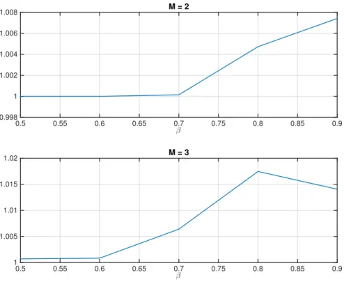
FIGURE1.1: Salient features of pairwise trades

addition to taxes discussed in section 2, when consumers meet the poorest producer, we also find taxation in meeting (1, 3), when the producer has one unit and the consumer has three, but only for very high β (of .9). So the main lesson is that with more divisibility of money traders are more conservative in terms of spending money and consumer taxes prove to be more efficient in terms of providing insurance.

Some basic effects of changes in the upper bound are displayed in Figure 1. The top two panels refer to the 4 bound, while the bottom two refer to the 2 bound. On the left we can see the effects of β on output and average payment in meeting (2, 2) with the 4 bound (top panel), and in meeting (1, 1) with the 2 bound (bottom panel). On the right, curves represent now the mean of the distribution of holdings and the ratio between average payment and output (called ‘price’) for the 4 bound (top panel) and the 2 bound (bottom panel).12

12_{Payment statistics used in Figure 1 are defined as the average transfer of money in meeting (2, 2) (for bound}

(39)

TABLE1.9: Outside money in pairwise meetings: core on β 0.9 0.8 0.7 0.6 0.5 m y/ λ(x) y/ λ(x) y/ λ(x) y/ λ(x) y/ λ(x) (0,1) 1.0007 / 0.18 (1) 1.0007 / 0.29 (1) 1.0067 / 0.50 (1) 1.0000 / 0.78 (1) 0.8377 / 1.00 (1) (0,2) 3.1900 / 1.00 (1) 3.3972 / 1.00 (1) 2.0209 / 1.00 (1) 1.2184 / 1.00 (1) 0.7794 / 1.00 (1) (0,3) 4.2274 / 1.00 (1) 3.3972 / 1.00 (1) 2.0209 / 1.00 (1) 1.2850 / 0.90 (2) 1.0000 / 0.90 (2) (0,4) 5.1675 / 1.00 (1) 2.2917 / 0.49 (2) 1.8818 / 1.00 (2) 1.6358 / 1.00 (2) 1.0194 / 1.00 (2) (1,1) 0.2947 / 0.14 (1) 0.2521 / 0.22 (1) 0.2364 / 0.37 (1) 0.1967 / 0.56 (1) 0.1473 / 0.81 (1) (1,2) 1.0000 / 0.49 (1) 1.0000 / 0.89 (1) 0.6372 / 1.00 (1) 0.3500 / 1.00 (1) 0.1810 / 1.00 (1) (1,3) 1.8766 / 1.00 (1) 1.1272 / 1.00 (1) 0.6372 / 1.00 (1) 0.3500 / 1.00 (1) 0.1810 / 1.00 (1) (1,4) 2.0553 / 1.00 (1) 1.1272 / 1.00 (1) 0.9035 / 1.00 (2) 0.4533 / 1.00 (2) 0.2274 / 1.00 (2) (2,1) 0.1571 / 0.13 (1) 0.1099 / 0.19 (1) 0.0793 / 0.30 (1) 0.0426 / 0.41 (1) 0.0269 / 0.58 (1) (2,2) 0.5333 / 0.43 (1) 0.4368 / 0.75 (1) 0.2663 / 1.00 (1) 0.1025 / 1.00 (1) 0.0464 / 1.00 (1) (2,3) 0.5333 / 0.43 (1) 0.4368 / 0.75 (1) 0.2663 / 1.00 (1) 0.1025 / 1.00 (1) 0.0464 / 1.00 (1) (2,4) 1.2423 / 1.00 (1) 0.5804 / 1.00 (1) 0.2663 / 1.00 (1) 0.1990 / 1.00 (2) 0.1017 / 1.00 (2) (3,1) 0.1197 / 0.12 (1) 0.0479 / 0.16 (1) 0.0209 / 0.23 (1) 0.0396 / 0.41 (1) 0.0337 / 0.61 (1) (3,2) 0.4076 / 0.41 (1) 0.1892 / 0.64 (1) 0.0898 / 0.97 (1) 0.0965 / 1.00 (1) 0.0553 / 1.00 (1) (3,3) 0.4076 / 0.41 (1) 0.1892 / 0.64 (1) 0.0927 / 1.00 (1) 0.0576 / 0.59 (1) 0.0509 / 0.92 (1) (3,4) 1.0007 / 1.00 (1) 0.2969 / 1.00 (1) 0.0927 / 1.00 (1) 0.0965 / 1.00 (1) 0.0553 / 1.00 (1) µ0 0.0720 0.1171 0.1862 0.2263 0.2695 µ1 0.3572 0.3708 0.3584 0.3164 0.2801 µ2 0.3437 0.2806 0.2450 0.2459 0.2415 µ3 0.1712 0.1605 0.1337 0.1163 0.1083 µ4 0.0559 0.0710 0.0767 0.0951 0.1006 v0 0.4514 0.0263 0.0089 0.0018 0.0013 v1 1.2638 0.5940 0.3948 0.2282 0.2253 v2 1.5692 0.7824 0.5166 0.3663 0.2738 v3 1.7538 0.8794 0.5675 0.3892 0.2861 v4 1.9027 0.9291 0.5851 0.4107 0.3010

λ(x)is the optimal probability of transfering x units of money (and paying x−1 units with probability 1−λ(x)).

Meetings (1, 1) and (2, 2) are important meetings in terms of their impacts on the dis-tribution of money for, respectively, bounds 2 and 4. Curves for output, representing con-sumption relative to first-best levels, indicate that the economy with 4 units has more trade going on. Curves for payments show that people save more for a large set of preferences with the 4 bound, an indication that the Inada condition has produced steeper value func-tions around 0 holdings. In this sense, money becomes more valuable (output doubles at high β).

With the 2 bound payments hit the ceiling of consumers’ holdings in meeting (1, 1) at low β such that positive inflation is optimal. Core effects are important for low β, confirm-ing what has been remarked above. When the core is off, output is smaller but both the meeting’s payment and the quantity of money vary little with β.

It is fair to say that the curve changing the most with the bound is the one reflecting opti-mal payments in these ‘critical’ meetings. Based on Figure 1, a reasonable conjecture is that output and payments vary less with the discount factor as the bound is increased further,

(40)

TABLE1.10: Outside money in pairwise meetings: core off β 0.9 0.8 0.7 0.6 0.5 m y/ λ(x) y/ λ(x) y/ λ(x) y/ λ(x) y/ λ(x) (0,1) 0.8856 / 1.00 (1) 0.7345 / 1.00 (1) 0.5969 / 1.00 (1) 0.4981 / 1.00 (1) 0.4084 / 1.00 (1) (0,2) 1.1316 / 1.00 (1) 1.1668 / 1.00 (1) 1.0299 / 1.00 (1) 0.8773 / 1.00 (1) 0.6305 / 1.00 (1) (0,3) 2.5093 / 1.00 (1) 2.2064 / 1.00 (1) 1.4570 / 1.00 (1) 0.9895 / 0.04 (2) 0.9058 / 1.00 (2) (0,4) 3.2446 / 1.00 (1) 2.2745 / 0.07 (2) 2.1144 / 1.00 (2) 1.4009 / 1.00 (2) 0.9058 / 1.00 (2) (1,1) 0.2266 / 0.12 (1) 0.1249 / 0.12 (1) 0.0718 / 0.11 (1) 0.0419 / 0.10 (1) 0.0254 / 0.09 (1) (1,2) 1.0007 / 0.55 (1) 1.0000 / 0.97 (1) 0.6574 / 1.00 (1) 0.4293 / 1.00 (1) 0.2745 / 1.00 (1) (1,3) 1.8325 / 1.00 (1) 1.0337 / 1.00 (1) 0.6574 / 1.00 (1) 0.4293 / 1.00 (1) 0.2745 / 1.00 (1) (1,4) 1.8325 / 1.00 (1) 1.0337 / 1.00 (1) 1.0000 / 0.84 (2) 0.6904 / 1.00 (2) 0.4473 / 1.00 (2) (2,1) 0.1137 / 0.09 (1) 0.0516 / 0.07 (1) 0.0254 / 0.06 (1) 0.0135 / 0.05 (1) 0.0082 / 0.05 (1) (2,2) 0.3530 / 0.27 (1) 0.2132 / 0.31 (1) 0.1227 / 0.30 (1) 0.0711 / 0.27 (1) 0.0419 / 0.24 (1) (2,3) 1.0000 / 0.76 (1) 0.6941 / 1.00 (1) 0.4099 / 1.00 (1) 0.2610 / 1.00 (1) 0.1728 / 1.00 (1) (2,4) 1.3126 / 1.00 (1) 0.6941 / 1.00 (1) 0.4099 / 1.00 (1) 0.2610 / 1.00 (1) 0.1728 / 1.00 (1) (3,1) 0.0464 / 0.05 (1) 0.0157 / 0.04 (1) 0.0060 / 0.03 (1) 0.0030 / 0.02 (1) 0.0015 / 0.02 (1) (3,2) 0.0965 / 0.09 (1) 0.0396 / 0.09 (1) 0.0172 / 0.08 (1) 0.0082 / 0.07 (1) 0.0045 / 0.06 (1) (3,3) 0.2378 / 0.23 (1) 0.1369 / 0.31 (1) 0.0868 / 0.41 (1) 0.0606 / 0.50 (1) 0.0411 / 0.57 (1) (3,4) 1.0000 / 0.98 (1) 0.4361 / 1.00 (1) 0.2132 / 1.00 (1) 0.1212 / 1.00 (1) 0.0711 / 1.00 (1) µ0 0.0361 0.0377 0.0365 0.0335 0.0307 µ1 0.2906 0.3165 0.3366 0.3443 0.3433 µ2 0.4432 0.4301 0.4341 0.4455 0.4580 µ3 0.2030 0.1893 0.1692 0.1558 0.1471 µ4 0.0271 0.0264 0.0236 0.0209 0.0209 v0 0.7894 0.2035 0.0706 0.0229 0.0068 v1 1.2715 0.5723 0.3489 0.2394 0.1754 v2 1.5437 0.0745 0.4745 0.3351 0.2489 v3 1.7387 0.8610 0.5527 0.3932 0.2951 v4 1.8896 0.9339 0.5934 0.4201 0.3141

λ(x)is the optimal probability of transfering x units of money (and paying x−1 units with probability 1−λ(x)).

indicating that more insurance is provided. This perhaps can explain that the quantity of money less than doubles as the bound is increased from 2 to 4: as the insurance problem is alleviated, the planner reduces the quantity of money, relatively, in order to improve the return of money (and the intensive margin of consumption).13

Confirming what we have seen with intermediation, the core requirement has a strong effect on exchange risk. This is quite evident in the relationship between β and the optimal distribution of money across tables. When the core is off (Table 10) the distributions do not change much with β and display a bell shape. When the core is on (Table 9), by contrast, reductions in β (and thus in saving rates) have a remarkable effect on the mass of people with low holdings of money, up to the point that the distribution approaches the uniform case. This is consistent with a strong velocity effect that makes expansionary policies sub-optimal. In addition, consumers in meeting (2, 4) spend more than one unit of money when

13_{Explaining why turning the core off leads to a higher quantity of money and taxation of poor consumers is}

more challenging. Focusing on poor consumers instead of richer ones helps with the return of money, which perhaps needs more attention when the quantity of money is increased.

Essays on monetary theory

D

T

Essays on Monetary Theory

Acknowledgements

Contents

List of Figures

List of Tables

Introduction

Chapter 1

A paradox of expansionary policies

1.1

Introduction

1.2

A preview

1.3

Adding more risk

1.4

Adding inflation

1.5

Measuring the savings friction