Theory of Product Differentiation in the Presence of the Attraction Effect

(1)

Theory of Product Differentiation in the Presence of the

Attraction Effect

∗

Efe A. Ok

†

Pietro Ortoleva

‡

Gil Riella

§

September 2011

Preliminary and Incomplete

Abstract

We apply the theoretical model of endogenous reference-dependence of Ok, Ortol-eva and Riella (2011) to the theory of vertical product differentiation. We analyze the standard problem of a monopolist who offers a menu of alternatives to consumers of different types, but we allow for agents to exhibit a form of endogenous reference depen-dence like the attraction effect. We show that the presence of such biases might allow the monopolist to overcome some of the incentive compatibility constraints of the stan-dard problem, leading the economy back towards the efficient equilibrium in which the monopolist extracts all the surplus. We then discuss welfare implications, showing that an increase in the fraction of customers who are subject to the attraction effect might not only increase the monopolist’s profits and total welfare, but consumer’s welfare as well.

JEL Classification: D11, L12, L15

Keywords: Attraction Effect, Reference-Dependence, Endogeneous Reference Forma-tion, Vertical Product Differentiation.

∗_{Various comments of Heski Bar-Isaac, Jean-Pierre Benoˆıt, Alessandro Lizzeri, Yusufcan Masatlioglu, and}

Debraj Ray have contributed to this work; we gratefuly acknowledge our intellectual debt to them. We are also grateful to the support of the C. V. Starr Center for Applied Economics at New York University.

†_{Corresponding Author}_{: Department of Economics, New York University, 19 West 4th Street, New York,}

NY 10012. E-mail: efe.ok@nyu.edu.

(2)

1 Introduction

In recent years a sizable literature in consumer psychology and in marketing has documented the presence and relevance of a specific form of systematic violation of rationality in choice: the so-called attraction effect, also known as the asymmetric dominance effect, or the decoy effect. In a nutshell, this effect could be described as the phenomenon according to which the introduction of an asymmetrically dominated alternative to a set might induce the agent to choose the dominating alternatives, possibly in violation of standard rationality. To illustrate, consider some decision maker who chooses between goods characterized by two attributes. Consider two alternatives of this kind, x and y, and suppose, as in Figure 1 (left), that x is better in one dimension, but y is better in the other one. Suppose that our agent chooses

y when only x and y are available – our decision maker aggregates the two attributes and picks y. Suppose now that a third (decoy) alternative z is added to the set, as depicted in Figure 1 (right): indeed this alternative is dominated by x, but it is not dominated by y. The attraction effect phenomenon corresponds to the situation in which the introduction of the alternative z leads the agent to choose x when x, y, and z are available, in violation of rationality.

This phenomenon was first documented by Huber, Payne and Puto (1982), and it was later confirmed in a large number of studies in very different environments.1

Importantly, it has been shown to play an important role also in field studies on actual supermarkets. In particular, Doyle et al. (1999) conducted experiments in a local grocery store in the UK. First, the authors recorded the weekly sales of the Brands X (the store’s own brand, Spar (420 g) baked beans) and Y (Heinz (420 g) baked beans) in the grocery store under study, and observed that Brand X received 19% of the sales in a given week, and Y the rest, even though Brand X was cheaper. Doyle et al. then introduced a third Brand Z (Spar (220 g) baked beans) to the supermarket, which was identical to Brand X in all attributes (including the price) except that the size of Brand Z was visibly smaller. The idea here is that Brand Z was asymmetrically dominated; it was dominated by X but not by Y. In accordance with the attraction effect, the authors observed in the following week that the sales of Brand X had increased to 33% (while nobody had bought Brand Z).

Despite the large evidence in support of the importance of the attraction effect in the

1_{The attraction effect is demonstrated in the contexts of choice over political candidates (Pan, O’Curry}

and Pitts (1995)), choice over risky alternatives (Wedell (1991) and Herne (1997)), medical decision-making (Schwartz and Chapman (1999) and Redelmeier and Shafir (1995)), investment decisions (Schwarzkopf (2003)), job candidate evaluation (Highhouse (1996), Slaughter, Sinar and Highhouse (1999), and Slaughter (2007)), and contingent evaluation of environmental goods (Bateman, Munro and Poe (2008)). While most of the ex-perimental findings in this area are through questionnaire studies, some authors have confirmed the attraction effect also through experiments with incentives (Simonson and Tversky (1992) and Herne (1999)).

(3)

Figure 1. Illustration of the attraction effect

market, perhaps due to the lack of a suitable model of consumer’s choice, to our knowledge the literature in economics contains no formal discussion of how such phenomenon might affect standard economic models: for example, whether a monopolist could exploit the attraction effect in the economy to extract more surplus; or if, and how, this would affect the bundles that she would offer. The goal of this paper is precisely to fill this gap: we study a standard model of vertical product differentiation, in which we assume that a fraction of the customers is potentially subject to the attraction effect.

We consider a standard model of vertical product differentiation, based on the one sug-gested by Mussa and Rosen (1978). A monopolist decides the (observable) price and quality of her goods, and she faces consumers who could be of different types, unobservable to her. In the standard model there are two types of consumers, Hight and Low, depending on their relative evaluation of price and quality. In our model, instead, there will be four types: for each type H and L, a fraction of customers is subject to the attraction effect. The monopolist knows the distribution of types in the population, and in particular she knows how many cus-tomers are subject to the attraction effect, but like in the standard model she does not observe the type of each consumer, and, therefore, she is unable to perfectly discriminate. Rather, like in the standard model, she will offer bundles of products targeting different types. Since a fraction of the consumers are subject to the attraction effect, the monopolist might choose to offer not only goods targeted at specific types, but also somedecoy goods, meant to attract the sales towards some more profitable bundles. Since such decoy bundles will never be sold – they must be dominated to be ‘decoy’ – we need to specify the cost that the monopolist incurs in producing them: we use the parameter γ to indicate whether the monopolist needs to produce one decoy bundle for every customer she wishes to attract (γ = 1), or she doesn’t need to produce it at all, since it’s never sold (γ = 0), or any case in between (γ ∈(0,1)).

(4)

not, and if there is, which one it is. When there is no reference point, then the agent acts fully rationally: she chooses the elements that maximize her utilityU in that set. If, however, the set S admits a reference point r(S), then the agent instead only looks at the available options that also belong to the attraction region of the reference point: she only looks at the options inS∩Q(r(S)). Amongst those, however, she is fully rational. For our implementation of the model, we assume that the utility function is identical to that of the original types, the attraction region of each element is the set of options that dominate it in both price and quality, and the reference map identifies a reference point if and only if there are dominated options in the set, the best of which acts as a reference point.

Our main findings are the following. First, we show that the monopolist will never want to exploit the attraction effect for consumers of the Low type: if she does, it is only to ‘attract’ customers of the high type. We then show that, as long as the cost of producing decoy options (γ) is not too high, or as long as the fraction of high types who are subject to the attraction effect is high enough, the monopolist will exploit the fact that a fraction of the high types is subject to the attraction effect. To this end, she will produce a decoy good, strategically placed to attract customers. In particular, we show that in the special case in which producing the decoy good is costless (γ = 0), and in which every high type is subject to the attraction effect, then the economy is back to efficiency: thanks to the attraction effect, the monopolist is able to perfectly segment the market, reach first best solution, and extractall the surplus. Finally, we analyze the welfare effects of an increase on the proportion of customers who are subject to the attraction effect. We show that in this case the profit of the monopolist increases, as does the total welfare of the economy. Moreover, there are parameter ranges in which also the consumer surplus increases: while the low types are always indifferent, the high types who are not subject to the attraction effect are actually better off; the only customers who loose welfare are those who become subject to the attraction effect – but for many parameter values, the former effect dominates the latter, leading to the situation in which, in expectations, for some parameter values customers would be better off the more of them are bounded rational.

Our model fits in the growing literature that applies to industrial organization choice models which depart from standard rationality. We refer to Spiegler (2011) for an excellent survey. Although to the best of our knowledge there is no such models that studies the consequences of the attraction effect, there are studies that analyze product differentiation in the presence of other forms of departure from standard rationality. Amongst them, Esteban and Miyagawa (2006) and Esteban, Miiyagawa and Shum (2007) study the case in which consumers are characterized by Self-Control preferences `a la Gul and Pesendorfer (2001). They show that if the high type’s marginal value for the quality of goods raises with the temptation, then the monopolist is able to achieve perfect discrimination, overcoming the incentive problems – as it happens in our paper. As opposed to our results, however, they use very different departures from rationality, and their approach is based on menus, which makes them depart from the standard model in a way that we don’t need.

(5)

2 The standard model of vertical product

differentia-tion: Mussa and Rosen (1978)

We begin our analysis by discussing the standard model of vertical product differentiation, de-veloped in Mussa and Rosen (1978). This model will serve as a benchmark for the subsequent analysis.

Consider a monopolistic market for a single good, where there are two types of consumers with distinct taste parameters about the quality of the product. The two types are H (for high) and L (for low), and we assume that they are evenly distributed in the society. Types

H and L evaluate the utility of one unit of the good of quality q≥0 at price p≥0 as

UL(p, q) := θLq−p and UH(p, q) := θHq−p,

where θH > θL > 0. For concreteness, we work here with a particular production technology

by confining ourselves to the case of quadratic cost functions. That is, we assume that the cost of producing a unit good of quality q ≥ 0 is q2

. The problem of the monopolist is then to choose quality levels qH, qL ≥ 0 and unit prices pH, pL ≥ 0 in order to solve the following

maximization problem:

Π∗ _{= max (}_p

L−q2L) + (pH −qH2)

such that UL(pL, qL)≥0,

UH(pH, qH)≥0,

UH(pH, qH)≥UH(pL, qL),

UL(pL, qL)≥UL(pH, qH).

In what follows we work with the parametric restriction θL > θ2H. This condition guarantees

the presence of a (unique) strictly positive solution for the monopolist’s problem, simplifying our analysis and allowing us to avoid the treatment of less interesting corner solutions. This solution has the first and third constraints binding and the optimal quality choices of the monopolist are found as:

qM R

H =

θH

2 and q

M R

L =θL−

θH

2 .

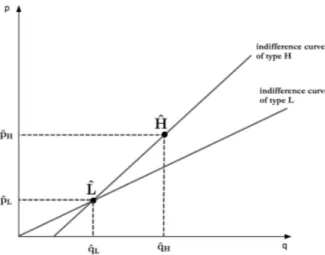
(The product produced by the monopolist for theHtypes is shown by ˆH in Figure 2, and that forLtypes as ˆL.) As it is common with this type of screening models, the solution is ‘efficient at the top,’ in the sense that qM R

H is the efficient (socially optimal) level of quality. On the

other hand, there is a downward distortion of the low valuation agent’s quality with respect to the first-best outcome. In what follows, we shall refer to the menu {(pM R

H , qHM R),(pM RL , qM RL )}

as the MR solution.2

2_{It is easily computed from the constraints of the problem that}

pM R H =

θ2

H

2 −(θH−θL)(θL− θH

2 ) and p

M R

L =θL(θL−

θH

(6)

Figure 2. Solution of the standard vertical product differentiation model.

3 The Reference-Dependent Model of Ok, Ortoleva and

Riella (2011)

The main departure from the standard model of this paper is to allow consumers to be subject to forms of endogenous reference-dependence such as the attraction effect. We model this using the model of Ok, Ortoleva and Riella (2011), which we now describe. Consider a fixed separable metric space X: we think of X as the universal set of all distinct choice alternatives. We defineX_{to be the collection of all compact subsets of} _X_{. An element}_S _ofX

is referred to as a choice problem or achoice situation. The model studies the choice behavior of an agent, and the following definition is basic.

Definition 1. A correspondence c:X⇒X is said to be a choice correspondence on X _if

∅ 6=c(S)⊆S for every S ∈X_.

We can now introduce the reference-dependent choice model. In what follows, we reserve the symbol ♦ for an arbitrary object that does not belong to X.

Definition 2. A reference-dependent choice model that represents a choice correspon-dence c is a triplet hU,r, Qi, where U is a continuous real function on X (utility function),

r : X _→ _X _{∪ {♦}} _{is a map (reference map), and} _Q _: _X _{∪ {♦}} ⇒ X is a correspondence

(attraction region) such that,

1. For any S∈X_,

c(S) = arg maxU(S∩Q(r(S))) (1)

2. r is a reference-map: for anyS ∈X _{we have} _r₍_S₎_∈_S _whenever _r₍_S₎₆₌_♦._{And for any}

x, y ∈X, r({x, y}) =⋄;

(7)

4. For any S, T ∈X _with _r₍_S₎_∈_T _⊆_S_{, and arg max}_U₍_S_∩_Q₍_r₍_S₎₎₎_∩_T ₆₌_∅_{, we have}

arg maxU(T ∩Q(r(T))) = arg maxU(T ∩Q(r(S))).

The interpretation is the following. Here U is interpreted as the utility function of the individual decision maker, free of any referential considerations. In particular, if the alter-natives have various attributes that are relevant to the final choice – these attributes may be explicitly given, or may have a place in the mind of the agent – then U can be thought as aggregating the performance of all the attributes of any given alternative in a way that represents the preferences of the agent.

In turn,r serves as the reference map that tells us which alternative is viewed by the agent as the reference for a given choice situation: given any choice problemS inX_,_{a reference map}

r on X _{either identifies an element} _r₍_S_{) of} _S_{, which we understand as acting as a reference}

point when solving this problem; or it declares that no element inS qualifies to be a reference for the choice problem – we denote this situation byr(S) = ♦,where the symbol♦represents the idea of ‘empty.’ Under this interpretation, the requirement that for anyx, y ∈X we have

r({x, y}) = ⋄ is related to the fact that the notion of “reference alternative” that we intend to capture is not related to, say, the status quo bias phenomenon. The latter notion would necessitate a default option to be thought of as a “reference” in dichotomous choice problems as well. As we mentioned in the introduction, the focus of the model of Ok, Ortoleva, Riella (2011) is on the notion of “reference” alternatives that are not desirable in themselves, but rather, affect the comparative desirability of other alternatives. Thus, the reference notion becomes meaningful in the present setup only when there are at least two alternatives in the choice situation at hand, in addition to the alternative designated as the reference point.

The interpretation of the correspondence Q is more subtle. For any ω ∈ X ∪ {♦}, we interpret the set Q(ω) as telling us which alternatives in the universal set X look “better” to the agentwhen compared to ω – it may thus make sense to call Q(ω) the attraction region of

ω. (For instance, if the agent deems a number of attributes of the alternatives as relevant for her choice, then Q(ω) may be thought of as the set of all alternatives that dominate ω with respect to all attributes.) Accordingly, we have Q(♦) = X (condition 3) – “nothing” does not attract the agent’s attention to any particular set of alternatives, so every one of them belongs to its attraction region.

Given these definitions, take any choice problem S ∈ X_. _{The agent either evaluates this}

problem in a reference-independent manner, or she identifies a reference point in S and uses this point to finalize her choice. In the former case,r(S) = ♦,so, by condition (3),Q(r(S)) =

X, which means that, in this case (1) reads

c(S) = arg maxU(S),

in concert with the standard theory of rational choice.3

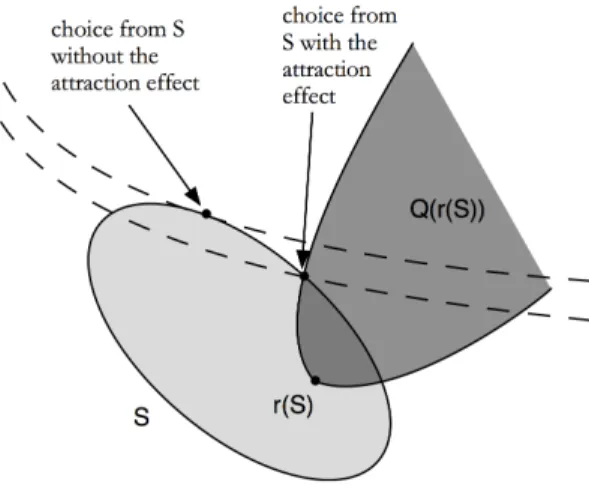
That is, when there is no reference point (r(S) = ♦), the agent behavior coincides with that of a standard agent. On the other hand, when there is a reference point (r(S)6= ♦), then the agent is mentally “attracted” to the elements of S that belong to Q(r(S)). It is “as if” she faces the mental constraint that

(8)

Figure 3. The Reference-Dependent Choice model of Ok, Ortoleva, Riella (2011).

her choices from S must belong to Q(r(S)) – and she disregards any option that does not belong to this set. As illustrated in Figure 3, however, within this constraint the agent acts fully rationally, and solves her problem upon the maximization of U,that is,

c(S) = arg maxU(S∩Q(r(S))).

Finally, the rationale for Condition (4) is the following. Without this condition, in general such a model would not at all restrict how the reference points of an agent relate to each other across varying choice situations. To illustrate, take a choice correspondence c on X _{that is}

represented by such a model hU,r, Qi, and suppose thatS is a choice problem in X_{such that}

r(S)6=♦ and x∈c(S). (2)

Then, x need not be a utility-maximizing alternative in S; it rather maximizes U over the subset of S that consists of all alternatives toward which the reference alternative r(S) “at-tracts” the agent (i.e. over S∩Q(r(S))). Now consider another choice problem T ∈ X _such

that

{x,r(S)} ⊆T ⊆S. (3)

The model hU,r, Qi does not put any restrictions on what would the reference point in T

be, and hence, on how the choice from T would relate to that from the larger set S. It may be that a new alternative r(T) now acts as a reference in T and an alternative y – whose utility may be significantly belowU(x) – is thus chosen by the agent due to this (i.e., because

y ∈Q(r(T)) and x /∈ Q(r(T))). Put differently, the arbitrariness of the r function allows for rather wild violations of the Weak Axiom of Revealed Preference (WARP), thereby taking away significantly from the predictive strength of the model hU,r, Qi.

(9)

4 Vertical Product Differentiation with the Attraction

Effect

4.1 General Discussion

We now apply the reference-dependent choice model described in the previous section to develop a model of vertical product differentiation, similar to the one described in Section 2, but in which at least a fraction of the consumers might be subject to the attraction effect. To simplify the exposition, and avoid the consideration of certain trivial cases, we shall carry out the condition from the MR model which guarantees an interior solution: we assume in what follows that θL> θ2H.

Suppose that some consumers in the market are subject to the attraction effect – we refer to these consumers as type AH or AL, depending on the fact that they are originally type

H or L. Since we allow for the contemporaneous presence of both consumers who are and consumers who are not subject to the attraction effect for each original type of consumer, we therefore have four types of consumers in this market: H, L, AH, and AL. Types H and

L are modeled as in the standard case, while types AH and AL will be modeled following

the model described in Section 3.4

We are going to make a small modification to the setup in the MR model. Now we are going to define X to be R2

+ × {0,1}. The idea is that the

alternatives have a third binary attribute on top of their prices and qualities. The main reason we are introducing this third attribute is to avoid some technicalities in the statement of the monopolist’s problem when some agents suffer from the attraction effect. As we have said, the choice behavior of typeAi consumers is modeled by means of a reference dependent choice

model hUAi,ri, Qi on the set X of all compact subsets of R

2

+× {0,1} as follows. First, we

posit that these consumers maintain the utility function that they had in their original type, that is, UAH = UH and UAL = UL. Second, we recall that a plausible interpretation of the

attraction region Q(ω) of a choice alternative ω is as the set of all alternatives that dominate

ω with respect to each attribute relevant for choice. This interpretation fits particularly well in the present setup. For a given alternative (p, q, b) we define the attraction region of (p, q, b) byQ(p, q, b) :={(s, t, v)∈_R2

+× {0,1}}:s≤p,t≥q and either both inequalities are strict or

v =b}∪{(0,0,0)}. As we have discussed before, the main reason we have introduced the third attribute to the setup now is to avoid some technicalities in the statement of the monopolist’s problem. If we had not done that, the maximum would not necessarily be attained in that problem. Notice that we also assume that the possibility of buying nothing (the option (0,0,0)) is always considered by the individual, represented by the fact that (0,0,0) ∈ Q(p, q, b) for any (p, q, b)∈_R2

+× {0,1}. 5

This is motivated by the fact that ‘not buying’ is a special option for the decision maker, which could always be considered. Moreover, since often purchases can be returned, we could imagine that if our decision maker were to purchase an option that she wouldn’t choose against (0,0,0), she could always return it – thus such sales should not be considered. It should be noted that if we were to drop this assumption, our results would be

4_{Since this model coincides with rational choice when}_{r(S) =}_♦_{for all}_{S, then we can also assume that}_all

types are modeled as in Section 3, but that for typesH andL we also haver(S) =♦for allS.

5_{Other choices for the correspondence}_Q_{that yield narrower attraction regions (and hence weaker attraction}

(10)

substantially different – as the monopolist would exploit the possibility of selling objects with a negative utility – but the main qualitative findings of our analysis would remain unaltered. Finally, we discuss the choice of ri. Recall that in the reference dependent choice model,

for a given set S, we can have ri(S) ∈ S only if there exists (p, q, b) ∈ S ∩Q(ri(S)) with

UAi(p, q) > UAi(ri(S)): a reference can come into play only if it attracts the attention of

the individual to some alternative that is strictly better than the reference itself. We then define r(S) as to be an arbitrary member of the dominated alternatives inS, and set it to ♦

(and hence posit reference-free behavior) if there is no such alternative. For concreteness, for any finite S, we shall taker(S) to be a bundle that maximizes UAi among all the dominated

alternatives in S (that is, all alternatives z ∈ S such that UAi(x) > UAi(z) for some x ∈

Q(z)∩S).6

This completes the specification of hUAi,ri, Qi,that is, the choice behavior of a consumer

who suffers from the attraction effect. It is easy to check thathUAi,ri, Qiis indeed a

reference-dependent choice model in the sense of Definition 3. We denote the choice correspondence that is represented by this model as cAi.

4.2 Stating the Problem

Now that we have specified the choice correspondence of the agents who suffer from the attraction effect, we can study the menu of bundles offered by the monopolist in the presence of such agents. We assume that for each i =L, H, a fraction αi ∈[0,1] of the i type agents

suffers from the attraction effect. We first observe that it is never going to be the case that the monopolist will want to offer a menu with more than six different goods. In fact, we can write the menu offered by the monopolist as{(pL, qL, bL), (pAL, qAL, bAL), (pRL, qRL, bRL),

(pH, qH, bH), (pAH, qAH, bAH), (pRH, qRH, bRH)}, where (pL, qL, bL),(pH, qH, bL) are the bundles

offered to the standardLandH types, (pAL, qAL, bAL),(pAH, qAH, bAH) are the bundles offered

to the bounded rational versions of those types, and (pRL, qRL, bRL),(pRH, qRH, bRH) are the

decoy goods used to attract the bounded rational agents of each type. Indeed there is no need for the monopolist to produce any additional product. We also understand that the bundle (0,0,0), representing the act of not buying, is always available.

Before writing the monopolist’s problem, we need to specify the cost of producing the decoy bundles (pRL, qRL, bRL) and (pRH, qRH, bRH). In fact, the main characteristic of these

bundles is that they need to be observable by the agents when they make their choice and, therefore, they need to be produced. At the same time, however, they are never sold – to act as a decoy, they must be dominated by some other option. Indeed, how costly they are depends on the specific market, and we will assume that if the monopolist wants a product to be seen by a fraction αi of the i type agents she has to incur a cost γαiqR2i. Indeed, γ

will be equal to 1 if the monopolist needs to produce one decoy bundle for each consumer she wants to attract, while it will be equal to 0 in the cases in which the bundle in fact need not be actually produced.7

Let S := {(pL, qL, bL), (pAL, qAL, bAL), (pRL, qRL, bRL), (pH, qH, bH),

6_{If there is more than one of such alternatives with the same utility pick the one with the smaller price. If}

they only differ in the third attribute pick the one withb= 0. If|S|=∞, letr(S) =⋄.

7_{We would have} _γ _{= 1 for a product sold in many locations, when the producer needs to offer a decoy}

(11)

(pAH, qAH, bAH), (pRH, qRH, bRH), (0,0,0)}. The monopolist’s problem in this case will be:

Π∗ _{= max} P

i=L,H

(1−αi) (pi−qi2) +αi(pAi −q

2

Ai)−γαiq

2 Ri

UH(pH, qH)≥max{UH(pL, qL), UH(pAL, qAL), UH(pAH, qAH)},

UL(pL, qL)≥max{UL(pH, qH), UL(pAL, qAL), UL(pAH, qAH)},

(pAL, qAL, bAL)∈cAL(S),

(pAH, qAH, bAH)∈cAH(S),

pAH, qAH, pAL, qAL, pH, qH, pL, qL, pRH, qRH, pRL, qRL ≥0.

(4)

where we understand that the reference bundles (pRi, qRi, bRi) will be set as (0,0,0) ifrAi(S) =

⋄. The first three constraints are in fact the standard participation and incentive compatibility constraints for the two groups of standard agents, H and L.8

Indeed, the interesting constraints here are the fourth and the fifth ones.

At first, this problem might appear difficult to analize. We will show, however, that it can in fact be reduced to a much simpler problem that we will be able to handle with the usual methods. The first step in this direction is to notice that the monopolist will not have any motivation to exploit the attraction effect for the low types: this result is contatined in the following proposition.

Proposition 1. The problem above has a solution, and any solution for the problem above satisfies (pL, qL) = (pAL, qAL).

The intuition for this proposition is extremely simple and provides many insights to what will follow. First, consider what are the advantages gained by a monopolist who does choose to exploit the attraction effect for some agents: it allows her to relax the incentive compatibility constraint for a portion of the agents. In fact, this is the only advantage gained by the monopolist from the use of the attraction effect: by forcing the agents to focus only on some particular set of options, she can reduce the incentive problems. At the same time, it does not allow the monopolist to overcome any participation constraint, since the bundle to which the agents are attracted to must still offer a non-negative utility – the option of not-buying is always available. Now, would a monopolist want to exploit the attraction effect for the low type agents? On the one side, this has some costs: she needs to produce a (potentially) costly reference bundle, which itself might create new incentive problems for the other types. On the other side, the advantage is that she can then relax the incentive compatibility constraint for this fraction of the lower types. But as it is the case in the MR solution, and as we shall see it is still the case here, in the optimum the incentive compatibility constraints of the low types arenot binding and, therefore, the monopolist has nothing to gain from relaxing them. Hence, she will never choose to exploit the attraction effect for the low types.

One should note that this result has some rather concrete marketing implications. In fact, this suggests that we should not see the exploitation of the attraction effect for the low types,

8_{As usual, we don’t have to write the participation constraint of the} _H _{type, since it is implied by the}

(12)

or, more in general, for the fraction of the agents whose incentive compatibility constraints are not binding in the solution.

Proposition 1 shows that we can concentrate our attention on the menus that do not use a decoy bundle for the low type bounded rational agents. That is, we can concentrate on the situations where the monopolist solves the following problem:

Π∗ _{= max} _p

L−q2L+

(1−αH) (pH −qH2) +αH(pAH −q

2

AH)−γαHq

2 RH

UH(pH, qH)≥max{UH(pL, qL), UH(pAH, qAH)},

UL(pL, qL)≥max{UL(pH, qH), UL(pAH, qAH)},

(pAH, qAH, bAH)∈cAH(S),

pAH, qAH, pH, qH, pL, qL, pRH, qRH ≥0.

(5)

where now S := {(pL, qL, bL),(pH, qH, bH),(pAH, qAH, bAH),(pRH, qRH, bRH),(0,0)}.

More-over, it turns out that we can simplify the problem even further: the following relaxed version of the problem has the same solutions of the problem above:

Π∗ _{= max} _p

L−q2L+

(1−αH) (pH −qH2) +αH(pAH −q

2

AH)−γαHq

2 RH

(pAH, qAH, bAH)∈cAH(S).

(6)

4.3 Solution

4.3.1 General Solution

The detailed solution of the problem at hand, divided in four cases, is discussed at length in the appendix. The main results, however, appear in the following two propositions.

Proposition 2. For any γ ∈ [0,1], there exists a α ∈ [0,1), such that it is strictly more profitable for the monopolist to use a decoy good than to use the MR solution if and only if

αH > α.

Proposition 3. For any αH ∈ (0,1), there exists a ¯γ > 0, such that using a decoy good is

strictly more profitable than the MR solution if and only if γ <γ¯.

Proposition 2 shows that, for any admissible values of θL, θH, and for any possible cost γ,

there exists a threshold α∈[0,1) such that the monopolist will want to exploit the attraction effect if, and only if, the proportion of the ‘high’ types who are subject to the attraction effect is above that threshold, i.e. if αH > α. In turn, sinceα <1, this means that, no matter what

the cost γ is, there always exists a proportion α such that the monopolist will find it strictly

(13)

The intuition of this result is simple. Recall that the attraction effect could be exploited by the monopolist to circumvent the incentive-compatibility constraints of the customers who are subject to it. The cost of doing this, however, is to pay the cost in producing the decoy good, and to add anadditional constraint for the customers who are not subject to it. Indeed if this latter group is small, the monopolist will accept this to extract more rent from those who are subject to the attraction effect. But if this group is large, then the situation is reversed, and the monopolist will not want to do so.

Proposition 3 discusses a similar argument for the cost γ: no matter what αH is, there

always exists a threshold ¯γ, strictly positive, such that the monopolist will want to exploit the attraction effect if, and only if the cost is below the threshold, i.e. γ <¯γ. In turn, since ¯γ

is strictly positive, this means that there always exists a cost low enough that the monopolist will want to exploit the attraction effect, no matter what αH is. In particular, if γ = 0, then

the monopolist will always want to the exploit the attraction effect, even if αH is arbitrarily

small.

The two propositions above show that at least when the cost of using a decoy good is not too large or the number of bounded rational agents is high enough, the monopolist will make use of such a strategy. We now show that except for a small range of the parameters θL and

θH the use of a decoy good will be profitable for the monopolist for all values of α ∈ (0,1)

and γ ∈[0,1].9

4.3.2 A special case: αH = 1 and γ = 0

An important special case of our analysis is the one in which αH = 1 and γ = 0: this is the

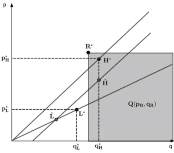
case in which every high type is subject to the attraction effect, and in which the monopolist incurs no cost in producing a decoy bundle – as it is the case for online sales. In this situation, as we can see from Case 1’s solution in the appendix, the monopolist can induce both the low type and the AH type to consume the efficient amount. This means that, as opposed to

standard screening models, the economy reaches the first best solution, with the monopolist extracting the entire surplus.

The reason is, in the MR model the monopolist could not reach the profits she would obtain were she able to segment the market because of the incentive compatibility constraints of the H type. But here, by exploiting only its attraction effect, the monopolist is able to overcome this incentive compatibility constraint, and therefore extract all the revenue from the consumers, reaching her first best solution. To do this, she only has to offer a decoy bundle (pRH, qRH, bRH) to prevent the incentive compatibility constraint of the H type to matter. And

since γ = 0, this decoy bundle can be produced at no cost, and, thus, the efficient solution can be attained. In particular, she could produce the following bundles, depicted in Figure 4:

q∗

AH :=

θH

2 , q

∗

L:=

θL

2 ,qRH =

θH +θL

2

with prices such that the participation constraints of both types H and L are binding, and

9_{It turns out that except for a small range of the parameters} _θ

L and θH the use of a decoy good will be

profitable for the monopolist for all values ofα∈(0,1) andγ∈[0,1].

Proposition 4. There exists 1

2 < a < a <1 such that if θL ≤aθH or θL ≥aθH, the monopolist will use a

(14)

Figure 4. Solution of the model whenαH= 1 and γ= 0.

any pRH > pAH. Hence, the following proposition.

Proposition 5. If all high type agents are subject to the attraction effect (αH = 1) and

the monopolist bears no cost in producing a bundle that is offered but never sold (γ = 0), then the monopolist is able to perfectly segment the market, the solution is efficient, and the monopolist extracts all the surplus.

4.4 Welfare Analysis

We now analyze the welfare implications of our model. In particular, we analyze how the welfare of each player in the economy changes as αH changes. For simplicity, we focus only

on the caseγ = 0. In this case, as we have seen, the monopolist will always choose to exploit the attraction effect and her profit will be higher than in the MR case. In particular, when

γ = 0, it can be checked that the expression for the profits of the monopolist comes from case 1 in the appendix and is given by

(θL−(1−αH) (θH −θL)) 2

4 +

θ2 H

4 ,

which is increasing and convex in αH. At the same time, this increase in profits happens

at the expenses of some of the consumers, who are now ”boundedly rational” since they are subject to the attraction effect. One should, therefore, expect the consumers to be worse off the higher αH is. But in fact, this is not always the case.

We now turn to analyze the consumer’s welfare. First of all, notice that the consumers of the low type always get the same welfare, equal to zero, no matter what αH is, since their

participation constraint is always binding for any parameter value. The key point of the analysis is what happens to the consumers of the high type. Indeed, if αH >0, they will be

divided into two groups,AH and H, exactly in anαH and (1−αH) proportions. The welfare

(15)

(θH −θL)(−

1

2(1−αH)(θH −θL) +

θL

2 ),

which is increasing and linear in αH. This means that each agent of the high type who does

not suffer from the attraction effect is actually better off the more people in her group do suffer from the attraction effect. The reason is rather simple: the less people of type H are in the market, the less the monopolist will want to distort her offerings to the other types in order to extract more revenue from them, and therefore the better off they are. Finally, we are left with customers of typeAH. It is immediate to see that any such agent is indifferent to

how many other agents suffer from the attraction effect: in fact, her participation constraint is always binding, and therefore her welfare is always zero.

The discussion above seems to suggest that, asαH increases, everybody is weakly better off:

the monopolists and type H are strictly better off, while type AH and type L are indifferent.

But clearly this is not the case: an increase in αH means that more and more agents do

suffer from the attraction effect, that is, some agents go from being typeH (where they had a positive payoff) to being typeAH (where they have a zero payoff). And if we wish to be able to

analyze the total welfare, we would need a way to compare their welfare as they change their status, but of course this is not trivial, as with their type they also change their preferences. In what follows, we will take the simplest approach: for those subjects who go from being typeHto being typeAH we consider their change in welfare as the difference in welfare of the

two types computed using their respective preferences. In our case this is particularly simple: since type AH receives a welfare zero, their change in welfare is the welfare they had as H,

which they loose becoming AH.10 This means that all such agents are actually worse off as

αH increases. In fact, they are the only ones loosing from the change.

We can now compute both the total welfare, and the aggregate consumer welfare. Let us start from the latter. Since agents of type L always receive zero, what changes is the aggregate welfare of the agents of the high type (H and AH).11 It turns out that, if θH

and θL are different enough, and if αH is small enough, their welfare is actually increasing

with αH.12 This means that, as long as αH is small, a consumer is actually better off if her

chances of being boundedly rational increase. This happens because the welfare increase of typesH more than compensates the welfare loss of some customers going from H toAH. Put

differently, the move towards efficiency, which takes place as αH increases, is such that, on

average, consumers are also better off. In turn, this means that in this parametric range, an increase in the bounded rationality of the agents (increase in αH) is actually leading to an

improvement in expected terms for each member of the economy, since both the monopolist 10_{Indeed other notions are possible, but here we are taking the most conservative one in terms of total}

welfare, i.e. we are taking the approach for which the welfare increases as little as possible asαH increases –

making our results of a welfare increase robust to other specifications. This approach, moreover, is justified by the fact that typeAH has indeed the possibility to buy the bundle that typeH buys, but she doesn’t do

so exactly because she is subject to the attraction effect. If, however, other bundles were not present, and she were offered only those two, she would instead buy the bundle that H buys, since there are no reference effects with only two options. Again this suggests that the utility lost from buyingH is exactly the welfare lost passing from beingH to beingAH.

11_{If the model is interpreted as there being only}_one _{agent, whose type is unknown to the monopolist, then}

what we now describe is theex-ante welfare of such customer,before she finds out her type.

12_{More precisely, the total consumer welfare is increasing in}_α_{as long as}_θ

(16)

Figure 5. Welfare changes withαH, computed withγ= 0,θL= 0.6,θH = 1 andαH∈[0,1].

and the high type agents are better off, while the low type agents are indifferent.

Finally, we consider the change in total welfare. It turns out that the total welfare is a strictly increasing and concave function ofαH. Part of this result is intuitive: since the higher

the proportion of agents who suffer from the attraction effect, the closer the market gets to the efficient allocation (which, again, is met when αH = 1). Graphically, an example of the

evolution of the welfare, both aggregate and of the specific players, is depicted in Figure 5 (where we have γ = 0, θL = 0.6 and θH = 1, while the MR solution is the one forαH = 0).

The discussion above can be summarized in the following proposition:

Proposition 6. If γ = 0:

1. The profit of the monopolist is a striclty increasing and convex function of αH.

2. The welfare of type L is unchanged with αH and is always equal to 0.

3. The welfare of type H who remain type H is increasing and linear in αH.

4. The welfare of type AH who remain type AH is constant and equal to zero.

5. If θL< 23θH, the expected welfare of the aggregate of types H and AH, as well as of the

consumers as a whole is increasing inαH as long as αH <

2θH−3θL

2θH₋2θL, decreasing for bigger

values, and it reaches a strictly lowest value at αH = 1. If θL≥ 23θH, it is a decreasing

function of αH.

6. Total welfare is a strictly increasing and concave function of αH.

Appendix: Product Differentiation with Attraction Effect

Solution of the Simplified Problem

(17)

Observation 1. If a menu satisfies the first three constraints of the problem above and it gives a payoff at least as great as theMRsolution, then it must necessarily satisfypAH−qAH2 −γqRH2 ≥pH−qH2. If such menu

gives a payoff strictly greater than theMRsolution, then the inequality above must be strict.

Proof of Observation 1. Suppose that a given menu satisfies all the constraints of the problem above and

pAH−q2AH−γq2RH

(≤)

< pH−qH2. But this implies that (pH, qH),(pL, qL) also satisfy the constraints of theMR

problem, which implies that

Π = pL−q2L

+αH pAH−qAH2

+ (1−αH) pH−q2H

−γαHqRH2

(≤)

< pL−qL2

+ pH−qH2

≤ΠM R

as we sought k

We now turn to discuss the solutions of the problem below. It can be divided in four cases:

Case 0. Suppose we add the constraintUH(pAH, qAH)≥UH(pL, qL) to the problem. The problem becomes

Π∗_{= max} _p

L−qL2+

(1−αH) (pH−q2H) +αH(pAH −q2AH)−γαHqRH2

UH(pAH, qAH)≥UH(pL, qL),

We work with the following relaxed version of the problem above:

Π∗_{= max} _p

L−qL2+

UH(pAH, qAH)≥UH(pL, qL).

It can be checked that all solutions of the problem above agree with the MR solution, in the sense thatqRH = 0

and (pL, qL), (pH, qH) = (pAH, qAH) are exactly the values found in that solution.

We have just shown that it is never going to be the case that the monopolist will exploit the attraction effect in order to make the individuals choose a good (pAH, qAH, bAH) such thatUH(pAH, qAH)≥UH(pL, qL). This

shows that the remaining interesting cases are the ones in whichUH(pAH, qAH)< UH(pL, qL)≤UH(pH, qH).

This can happen only ifQ(r_AH_(S))_∩_S ₌_{_(p_AH_{, q}_AH_{, b}_AH_),_(p_RH_{, q}_RH_{, b}_RH_),_(0,₀₎_}_{. This allows us to write}

the problem as

Π∗_{= max} _p

L−qL2+

pAH ≤pRH, qAH ≥qRH andUH(pAH, qAH)≥0,

pH ≥pRH or qH ≤qRH,

pL≥pRH orqL≤qRH.

Notice that in writting the problem above we are using the fact that the monopolist can use the third attribute to decide if an alternative that weakly dominates the reference with respect to the first two attributes belongs or not toQ(r_{(S)). We can divide the problem above in three cases.}

(18)

the following problem:

Π∗_{= max} _p

L−qL2+

qH ≤qRH,

qL≤qRH.

In what follows we work with the following relaxed version of the problem above

Π∗_{= max} _p

L−qL2+

such that pL−θLqL≥0,

pH−θHqH≥pL−θHqL,

pAH −θHqAH ≥0,

qH ≤qRH,

qL≤qRH.

It is easy to see that the first three constraints must be binding. The problem reduces to

Π∗_{= max} _θ

LqL−qL2+

(1−αH) (θHqH−(θH−θL)qL−qH2) +αH(θHqAH−q2AH)−γαHqRH2

such that qH ≤qRH,

qL≤qRH.

It is not hard to see that the first constraint must be binding.13 _{We can write the problem above as}

Π∗_{= max} _θ

LqL−qL2+

(1−αH) (θHqH−(θH−θL)qL−qH2) +αH(θHqAH−q2AH)−γαHqH2

such that qL≤qH.

The solution for this problem is

qL=

θL−(1−αH) (θH−θL)

2 ,

qH =

1−αH

1−αH+γαH

θH

2 ,

qAH =

θH

2 , if

γ≤

h

1−αH+ (1−αH)2

i

(θH−θL)

αH[θL−(1−αH) (θH−θL)]

,

and

qL=qH =

2−αH

2−αH+γαH

θL

2 ,

qA=

θH

2 , otherwise. The monopolist’s profit is

Π = (θL−(1−αH) (θH−θL))

2

4 +

1−αH+γα2H

1−αH+γαH

θ2

H

4 ,

13_{If this was not true we would have} _q

H = θH₂ < qRH. Independently of the value of qL, a deviation to

ˆ

(19)

in the first case and

Π =αH

θ2

H

4 +

(2−αH)2

2−αH+γαH

θ2

L

4 ,

in the second case. One can check that both solutions satisfy all the constraints that were ignored in order to get to the final simplified problem.

Case 2. Now suppose that we impose that the constraintspH ≥pRH andqL ≤qRH are satisfied. We first note

that the precise value ofpRH is not really important for the problem, all that matters is that it lies between

pAH and pH, so we can collapse the constraintspAH ≤pRH andpRH ≤pH into pAH ≤pH. Also, it is clear

that the solution will necessarily haveqRH =qL. We are left with the following problem:

Π∗_{= max} _p

L−qL2 +

(1−αH) (pH−qH2) +αH(pAH−qAH2 )−γαHq2L

UH(pAH, qAH)≥0,

pH ≥pAH,

qAH ≥qL.

We look to the following relaxed version of the problem above:

Π∗_{= max} _p

L−qL2 +

(1−αH) (pH−qH2) +αH(pAH−qAH2 )−γαHq2L

such that θLqL−pL≥0,

θHqH−pH ≥θHqL−pL,

θHqAH −pAH ≥0,

pH ≥pAH.

It is easy to see that all four constraints must be binding, which gives us the following simplified problem:

Π∗_{= max} _θ

LqL−qL2+

(1−αH) (θHqH−(θH−θL)qL−q2H) +αH(θHqAH −qAH2 )−γαHq2L

such that θHqAH =θHqH−(θH−θL)qL.

The solution for such problem is

qL=

_θ

L−(1−αH) (θH−θL)

2

/ 1 +γαH+

αH(1−αH) (θH−θL)2

θ2

H

!

,

qH=

θH

2 +

αH(θH−θL)

θH

qL,

qAH =

θH

2 −

(1−αH) (θH−θL)

θH

qL,

and the monopolist’s profit is

Π∗₌ θ2H

4 + ((2−αH)θL−(1−αH)θH)qL− 1 +γαH+

αH(1−αH) (θH−θL)2

θ2

H

!

qL2.

(20)

Case 3. Suppose now that we impose that the constraintpRH ≤pLis satisfied. We are left with the following

problem:

Π∗_{= max} _p

L−qL2+

pH ≥pRH or qH ≤qRH,

pL≥pRH.

We work with the following relaxed version of the problem above:

Π∗_{= max} _p

L−qL2+

such that θLqL−pL≥0,

θHqH−pH≥θHqL−pL,

θHqAH−pAH ≥0,

pAH ≤pL,

qAH ≥qRH.

Clearly, the solution for the problem above will haveqRH = 0, and given thatqAH <0 will never be optimal,

the constraintqAH ≥qRH is automatically satisfied. With this result at hand it is clear that the first three

constraints will be binding. In fact one can check that the fourth constraint will also be binding, which gives us the following problem:

Π∗_{= max} _θ

LqL−q2L+

(1−αH) (θHqH−(θH−θL)qL−q2H) +αH(θHqAH−qAH2 )−γαHq2RH

such that θHqAH =θLqL.

The solution for such problem is

qL=

θH

2

θH(2θL−(1−αH)θH)

θ2

H+αHθ2L

,

qAH =

θH

2

θL(2θL−(1−αH)θH)

θ2

H+αHθ2L

,

qH =

θH

2 , and the monopolist’s profit is

Π = θ

2

H

4

(2θL−(1−αH)θH)2

θ2

H+αHθL2

+(1−αH)θ

2

H

4 .

One can check that all the constraints that were ignored in order to get to the simplified problem above are satisfied by this solution.

Proof of Proposition 1.

Consider the following relaxed version of the problem in the main text

Π∗_{= max} P

i=L,H

(1−αi) (pi−qi2) +αi(pAi−q2Ai)−γαiq2Ri

UH(pH, qH)≥max{UH(pL, qL), UH(pAL, qAL)},

UL(pAL, qAL)≥0,

(21)

We note that (pRL, qRL, bRL) does not affect any of the constraints of the problem above, so clearly any solution

for the problem above must satisfy (pRL, qRL) = (0,0). Also, since (pL, qL) and (pAL, qAL) are subject to the

same restrictions, we can use the concavity of the objective function together with the convexity of the restriction set to show that any solution to the problem above must satisfy (pL, qL) = (pAL, qAL). This allows

us to concentrate on the following simplified version of the problem above:

Π∗_{= max} _p

L−qL2+

We have already shown that the problem above always has a solution that satisfies all the restrictions of the original problem. k

By Proposition 1 and the solution for the simplified problem, we know that the solution of the original problem always agrees with the solution of the simplified problem.

Let’s first show that for any θL, θH > 0 and γ = 1, if αH is big enough, then the simplified problem

is strictly more profitable than theMR case. Observe that in this case the payoff in Case 2 whenαH →1

converges to

ΠCase2_→ θH2

4 + θ2

L

8 . Similarly, the payoff in Case 3 whenαH →1 converges to

ΠCase3_→ θH2

4 4θ2

L

θ2

H+θ2L

.

Suppose that the limit of the payoff in Case 2 is smaller than the payoff in theMR solution, that is,

θ2 H 4 + θ2 L 8 ≤

θL−

θH 2 2 +θ 2 H 4 .

Leta= θL

θH. The expression above is equivalent to

7a2

8 −a+ 1 4 ≥0.

On the other hand, the limit of the payoff in Case 3 is strictly larger than the payoff in theMR solution if, and only if,

a4₋_a3₊a2

2 −a+ 1 2 <0. Since one is a root of the polynomial above anda∈ 1

2,1

, the condition above will be true if and only if

a3+a 2−

1 2 >0.

Finally, we note that the polynomial 7a2

8 −a+ 1

4 has one root in 0, 1 2

and another root in 3₄,1

. On the other hand the polynomiala3₊a

2 − 1

2 has a single root which is located in 1 2,

3 4

. Moreovera3₊a

2− 1 2 >0

ifais greater than this root. So whenever we have that Case 2 gives a profit smaller than theMR solution in the limit we must necessarily have that Case 3 gives a profit strictly greater than theMR solution whenαH

approaches 1. We conclude that there always existsαH such that ΠProblem (2) >ΠM R and this is obviously

also true when γ <1. Define α:= inf

αH: ΠProblem (2)>ΠM R . By what we have just provedα is

well-defined and it is easy to see that ΠProblem (2)_≤_ΠM R_when_α

(22)

we show that for any αH > α, ΠProblem (2) > ΠM R. For that pick any α∗ > α. By construction we know

that there exists ˆα∈[α, α∗_{) such that when}_α

H = ˆα, ΠProblem (2) >ΠM R. By observation 1 we know that

this implies thatpA−q2A−γqR2 > pH−qH2. But then, if the monopolist continues to offer this same bundle

whenαH =α∗, all the constraints will still be satisfied and she is going to make a higher profit than before.

Consequently, the solution whenαH =α∗ gives a strictly higher profit than theMR solution. This completes

the proof of the proposition. k

For any αH ∈ (0,1), Case 1 gives a payoff strictly higher than the MR solution when γ = 0. So define

¯

γ:= sup

γ: ΠProblem (2)_>_ΠM R _{. By what we have just discussed ¯}_{γ >}_{0 and, moreover, it is easy to see that}

when γ= ¯γ we must necessarily have ΠProblem (2) _≤_ΠM R_{. It only remains to be shown that for any} _{γ <}_γ_¯

the best attraction effect solution is necessarily strictly better than the MR solution. For that, let γ∗ _<_γ._¯

By construction there exists ˆγ ∈ (γ∗_,_{γ] such that using the attraction effect is strictly better than the}_¯ _MR

solution. But then it is clear that this same solution would also be strictly better than theMR solution for a smallerγ. k

References

Ariely, D. and T. Wallsten (1995), “Seeking Subjective Dominance in Multi-Dimensional Space: An Expla-nation of the Asymmetric Dominance Effect,” Organizational Behavior and Human Decision Processes, 63, 223-232.

Bateman, I., A. Munro, and G. Poe (2008), “Decoy Effects in Choice Experiments and Contingent Valuation: Asymmetric Dominance,”Land Economics, 84, 115-127.

Bhargava, M., J. Kim, and R. Srivastava (2000), “Explaining Context Effects on Choice Using a Model of Comparative Judgement,”Journal of Consumer Psychology, 9: 167-177.

Burton, S. and G. Zinkhan (1987), “Changes in Consumer Choice: Further Investigation of Similarity and Attraction Effects,”Psychology and Marketing, 4: 255-266.

Doyle J., D. O’Connor, G. Reynolds, and P. Bottomley (1999), “The Robustnes of hte Asymmetrically Domi-nated Effect: Buying Frames, Phantom Alternatives, and In-Store Purchases,”Psychology and Marketing, 16, 225-243.

Esteban, S. and E. Miyagawa (2006), “Temptation, Self-Control, And Competitive Nonlinear Pricing,” Eco-nomic Letters, 90, 348-355.

Esteban, S., Miyagawa, E. and M. Shum (2007), “Nonlinear Pricing with Self-Control Preferences,”Journal of Economic Theory, 135, 306-338.

Gul, F. and W. Pesendorfer (2001), “Temptation and Self-Control,”Econometrica, 69, 1403-1435.

Herne, K. (1997), “Decoy Alternatives in Policy Choices: Asymmetric Domination and Compromise Effects,”

European Journal of Political Economy, 13, 575-589.

Herne, K. (1999), “The Effects of Decoy Gambles on Individual Choice,”Experimental Economics, 2, 31-40.

Highhouse, S. (1996), “Context-Dependent Selection: Effects of Decoy and Phantom Job Candidates,” Orga-nizational Behavior and Human Decision Processes, 13, 575-589.

Huber, J., J. Payne, and C. Puto (1982), “Adding Asymmetrically Dominated Alternatives: Violations of Regularity and the Similarity Hypothesis,”Journal of Consumer Research,9, 90-98.

(23)

Lehman, D. and Y. Pan (1994), “Context Effects, New Brand Entry and Consideration Sets,” Journal of Marketing Research,31, 364-374.

Mishra, S., U. Umesh, and D. Stem (1993), “Antecedents of the Attraction Effect: An Information Processes Approach,”Journal of Marketing Research,30, 331-349.

Mussa, M. and S. Rosen (1978), “Monopoly and Product Quality,”Journal of Economic Theory, 18: 301-317.

Ok, E., Ortoleva, P. and Riella, G. (2009), ”Revealed (P)Reference Theory,” mimeo. New York University.

Pan, Y., S. O’Curry, and R. Pitts (1995), “The Attraction Effect and Political Choice in two Elections,”

Journal of Consumer Psychology, 4: 85-101.

Ratneshwar, S., A. Shocker, and D. Stewart (1987), “Toward Understanding the Attraction Effect: The Implications of Product Stimulus Meaningfulness and Familiarity,”Journal of Consumer Research, 13: 520-533.

Redelmeier, D. and E. Shafir (1995), “Medical Decision Making in Situations that Offer Multiple Alternatives,”

Journal of American Medical Association, 273: 302-305.

Richter, M.(1966), “Revealed Preference Theory,”Econometrica,34, 625-645.

Sagi, J. (2006), “Anchored Preference Relations,”Journal of Economic Theory, 130, 283-295.

Schwartz, R. and G. Chapman (1999), “Are More Options Always Better? The Attraction Effect in Physicians’ Decisions about Medications,”Medical Decision Making, 19: 315-323.

Schwarzkopf, O. (2003), “The Effects of Attraction on Investment Decisions,”Journal of Behavioral Finance,

4, 96-108.

Sen, S. (1998), “Knowledge, Information Mode, and the Attraction Effect,” Journal of Consumer Research, 25: 64-77.

Shafir, S., T. Waite, and B. Smith (2002), “Context Dependent Violations of Rational Choice in Honeybees (Apis Mellilea) and Gray Jays (Perisoreus Canadensis),”Behavioral Ecology and Sociobiology, 51, 186-187.

Simonson, I. (1989), “Choice Based on Reasons: The Case of Attraction and Compromise Effects,” Journal of Conflict Resolution, 16: 158-175.

Simonson, I. and S. Nowlis (2000), “The Role of Explanations and Need for Uniqueness in Consumer Decision Making: Unconventioanal Choices based on Reasons,”Journal of Consumer Research, 27, 49-68.

Simonson, I. and A. Tversky (1992), “Choice in Context: Tradeoff Contrast and Extremeness Aversion,”

Journal of Marketing Research, 29, 281-295.

Sivakumar, K. and J. Cherian (1995), “Role of Product Entry and Exit on the Attraction Effects,”Marketing Letters, 29: 45-51.

Slaughter, J., (2007), “Effects of Two Selection Batteries on Decoy Effects in Job Finalist Choice,”Journal of Applied Social Psychology, 37, 76-90.

Slaughter, J., E. Sinar, and S. Highhouse (1999), “Decoy Effects and Attribute Level Inferences,”Journal of Applied Psychology, 84, 823-828.

Spiegler, R.,Bounded Rationality and Industrial Organization, Oxford University Press, Oxford, 2011.