ANALYSIS OF EQUILIBRIUM IN INDUSTRIAL VARIABLES
THROUGH ERROR CORRECTION MODELS
Adriano Souza1, Francisca Souza1, Rui Menezes2
1
Department of Statistics, Department of Industrial Engeneering UFSM (BRAZIL)
2
Department of Quantitative Methods, ISCTE – IUL (PORTUGAL)
E-mails: [email protected], [email protected],
ABSTRACT
This research aimed to evaluate the relationship between variables of the temperature adjustment and the percentage of heating in the molding oven of the Polyethylene Terephthalate Resin (PTR) used in the manufacture of the preform of two-liter bottles. It also investigated the direction of causality between these variables in order to determine how an external shock is transmitted to the system. Vector Error Correction (VEC) methodology was used to carry out this study. It was possible to identify the variable to be monitored and estimate the minimum time for the system to reach the stability of the oven temperature.
Key words: Quality control, vector autoregression, vector error correction model, response-impulse
variable, industrial oven temperature.
1. INTRODUCTION
The Statistical Process Control (SPC) uses the measurements obtained during the process to monitor and find changes that may be occurring without prescribing a control action. On the other hand, the Engineering Process Control (EPC) uses measurements of the process to reveal its future behavior, which, consequently, makes it possible to prescribe changes in variables to make them as close as possible to the desired target [1].
To apply SPC some assumptions are required in order to implement control charts. The sample data to be analyzed must come from a population that follows a Normal distribution and is independent and identically distributed (i.i.d.). Furthermore, it is important to know how to use EPC methodology, i.e., it is necessary to find the mathematical model that best represents the productive process thus this model serves as a guide in the future process. This way, it is possible to correct a change introduced in the process in order to maintain the production as close as possible to the model proposed.
For the interpretation of a productive process, the variables under analysis should be stationary because in such conditions any deviation from the target value established would be more easily detected. If the process is non-stationary it is likely to continue being like that, obeying the second law of thermodynamics. According to [2], the law of entropy or disorganization shows that the process only returns to an equilibrium condition due to the occurrence of an external action. This situation is corroborated by [3]. According to [4], the trend followed by variables such as temperature, pressure and density in isolated systems can be gradually increased until reaching a state of equilibrium.
The application of ARIMA models has been known for a long time in industrial area in the division of quality control; however, they present the disadvantage of the modeling stage when the process is not stationary. In order to make the process stationary, it is necessary to use differentiations in the series. According to [5], when this step is performed, the long-term properties that may be present in the series are lost. This way, conclusions on the long-run equilibrium of the system are not obtained since only short-term information is retained in different variables.
Time series that are non-stationary may present a dynamic common movement which deserves to be investigated. Therefore, an additional step is given in relation to ARIMA models. The relations of short and long run are investigated separately through a more complete autoregressive model called error correction model [6], [7]; [5], [8].
The purpose of this research was to evaluate the relationship between the variables of the temperature adjustment (TA) and the percentage of heating (PH) in the molding oven of Polyethylene Terephthalate Resin (PTR) in the stage of manufacturing the preform into a two-liter bottle. Moreover, the impulse response and the direction of causality between these variables were investigated in order to determine how an external action is transmitted in the entire system and how long it takes to be carried out.
The methodology is presented in Section 2, the characterization of the data in Section 3, and results, discussion, and conclusions in Section 4.
2. METHODOLOGY
The methodological steps for the analysis of the behavior of the TA and PH variables in the molding oven are described below.
1. Initially, the time series are tested in relation to stationarity aiming to verify the presence of unit roots through the Augmented Dickey-Fuller (ADF) – (1979), Elliott-Rothenberg-Stock (ERS) – (1996) and Kwiatkowski-Phillips-Schmidt-Shin (KPSS) – (1992) tests according to [9] and [10].
2. After the unit root is detected with the same order of integration d, the long-term relationship is estimated to identify the common trajectory between the variables. To determine if the variables are indeed
co-integrated, we used the residuals êt from the long-term relationship. If the residuals are stationary we can say, for
instance, that sequences or series are co-integrated of order (1,1). The series are called variables I (1) according to [12]. This uniequational procedure is known in literature as the test of Engle-Granger (EG).
Engle and Granger (1987) show that the elements (vectors) of Xt are said to be cointegrated of order (d, b),
denoted by Xt ≈ CI (d,b) if:
i) All elements of Xt are integrated of order d, i.e., I (d);
ii) There is a non zero vector, β, where ut = X
`
t β ≈ I(d-b), b > 0.
The first condition says to establish an error correction model all variables in study must have the same order of integration (d), if so they are non stationary and possibly will be co-integrated. The second condition says the variables enter in a long term relationship, which shows a joint movement. This commom movement derives from a stochastic trend and not from a spurious relationship between two random walk processes [5].
3. If the variables are co-integrated, we can estimate a relationship among them called error correction model, which is based on the residuals of the equation of equilibrium (or long term). Using the nomenclature of [9]
and considering the variables Yt and Zt, we have:
∆ = + ( − ) + ( )∆ + ( )∆ +
1)
In eq. (1) the endogenous variable of the error correction model is Yt (similar to the long-term equation
which is normalized to Yt). However, in many situations there is no reason to set a priori which of the variables in
the model is endogenous, since both variables may be simultaneously endogenous. This situation occurs when in the system there are mutual interactions among the forces that compose it. Thus, another equation may be
specified where now Zt appears as the endogenous variable in the model. The combination of these equations in
the estimation of the model originates what is called a model VEC (Vector Error Correction).
∆ = + ( − ) + ( )∆ + ( )∆ + (2)
In the system, β1 is the co-integration parameter, and are white noise residual, and α's are the model
parameters. The variable linear combination in levels is replaced by residuals estimated in the long term equation.
∆ = + ê + ( )∆ + ( )∆ + (3)
∆ = + ê + ( )∆ + ( )∆ + (4)
The error correction model is a VAR model in first differences and the OLS estimator can be used to make the parameter estimative, otherwise the near VAR estimator should be used.
4. The number of lags which is needed to be incorporated in the error correction model is determined by Akaike information criteria (AIC) and Schwarz (SBC) [6].
)
/
(
2
)
/
(
2
l
T
k
T
AIC
(5)T
T
k
T
l
SBC
2
(
/
)
log(
)
/
(6)where T is the sample size, l is the value of the log likelihood function and k is the number of estimated parameters.
5. In order to determine the number of co-integrating vectors two important tests are used, namely trace statistic and maximum eigenvalue, as explained by [12] [13], [14], [15] [17] and [16].
The H0 represents the number of cointegrating vectors lower than or equal to r; and the alternative
hypothesis H1: represents the number of co-integrating vectors greater than r.
λ (r) = −T ln(1 − λ ) (7)
Since the maximum eigenvalue test has the following hypotheses: H0: The number of cointegrating vectors
is equal to r, and H1: The number of cointegrating vectors is equal to r +1.
( , + 1) = − ln(1 − ) (8)
where, are the eigenvalues obtained from matrix π, which represents the coefficients of the vectors of long-term error correction (for details, see [9], and T is the number of observations.
If the values of these statistics are greater than the critical value, the null hypothesis of no-cointegration is rejected. The critical values of trace test and maximum eigenvalue test are reported by [18].
6. The fitted model has its adequacy accomplished by means of diagnostic tests, where the white noise characteristic is searched. In this stage we also verified the impulse response of a variable in another one. The Choleski decomposition method was used and the impulses considered orthogonal. Thus, the reaction that one variable causes in the other, and the time required for the system to achieve the stability after an external shock are found.
7. Finally the Granger causality test as proposed by [14] is applied.
The goal is to check the direction of causality using Granger causality test [19] defined as follows: X2t
Granger causes X1t if ceteres paribus, the values passed of X2t help improve the current forecast of X1t as
discussed by [8].
It should be noted that to carry out this test the variables involved should be provided from a stochastic process, stationary or not, and that the future cannot cause the past. The specification of this test can be carried out considering the autoregressive distributed lag ADL (p, q) expression.
= + , + , + (9)
where, Xit (i = 1,2) denotes the variable i at time t, captures the autocorrelation in extended X1t, measures the
relationship between variables, and is a white noise disturbance. It is said that X2t Granger causes X1t, where the
null hypothesis of all parameters are simultaneously zero, or rejected. The direction of causality may be
unidirectional or bidirectional. In this case, we say that there is a feedback relationship.
Thus, this methodology is used to accomplish the main objective of this study. This way, it is possible to determine the time that a variable takes to reach equilibrium, and monitor its effect. The time to reach equilibrium in the productive process is important to help to predict the production process and identify the variable that should be given greater attention in the stage of the process monitoring.
3. DATA
The study was performed in the stage of making the preform of PTR, which has 54 g of weight, 152 mm long, and 22 mm in diameter in the neck and 29 mm in diameter in its body. After heating and expanding in the molding oven it is transformed into a 2 liter plastic bottle.
The main variables that affect the process are TA and PH in the molding oven, which has a direct relationship with the product quality. We collected 202 observations taken at one hour intervals in three shifts per day of an industrial production and bottling of soft drinks in the stage of molding.
4. RESULTS AND DISCUSSION
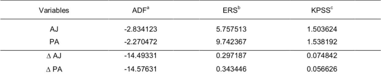
To test the stationarity of the series we used the ADF - (1979) and ERS - (1996) tests, where the null hypothesis that the variable has a unit root - I (1) was not rejected. Our results are corroborated by the results of the KPSS – (1992) test as shown in Table 1. The non-stationary series in level become stationary after the first difference thus there must be a long-term equilibrium and consequently the incorporation of error correction mechanisms.
Table 1. Unit root tests ADF, KPSS and ERS for the variable adjustment of temperature
and percentage of oven heating molding
Variables ADFa ERSb KPSSc
AJ -2.834123 5.757513 1.503624
PA -2.270472 9.742367 1.538192
AJ -14.49331 0.297187 0.074842
PA -14.57631 0.343446 0.056626
Note: Critical values in level of MacKinnon (1996): -3.462901 a (1%); -2.875752 a (5%) e -2.574462 a (10%). b Elliott-Rothenberg-Stock (1996 table 1): 1.910800 a (1%), 3.170900 a (5%) and, in level 4.331500 a (10%). c Kwiatkowski-Phillips-Schmidt-Shin(1992): 1.503624 a (1%), 0.739000 a (5%) e 0.347000 a (10%). In first differences MacKinnon (1996): 1.910800 a (1%); 3.170900 a (5%) e 4.331500 a (10%). b Elliott-Rothenberg-Stock (1996 table 1): 1.910400 a (1%), 3.170450 a (5%) e 4.330750 a (10%). c Kwiatkowski-Phillips-Schmidt-Shin (1992): 0.739000 a (1%), 0.463000 a (5%) e 0.347000 a (10%);
represents the series in first diferences.
Since the series in level are not stationary, and stationary in first difference, there must be a long-term equilibrium that deserves to be investigated by incorporating an error correction mechanism (ECM).
The ECM is useful in continuous manufacturing processes such as chemicals, where controllable factors as temperature, pressure, velocity of the flow in pipe can be controlled to achieve a particular quality characteristic.
According to [20], if there is a relationship between two variables, where one can be manipulated to cause an influence in the other to achieve a state of control and are measured at equidistant spaces of time, the effect of
a simple change in control variable may have its effect dissipated for several subsequent periods of time. Thus, it is important to find the time or delay that this action is performed. Furthermore, it is important to find the period in which the equilibrium occurs.
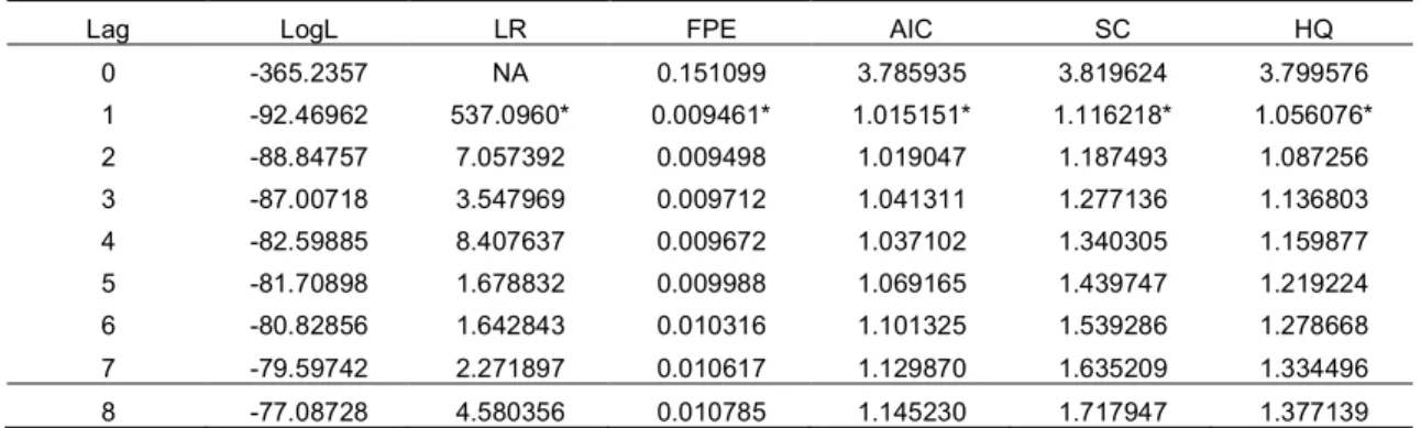
The VAR model is justified based on the need to analyze the dynamic impact of random disturbances in the system variables. Before you check the existence of the co-integrating vector it is important to determine the number of lags to be used in vector autoregressive (VAR), as shown in Table 2.
Table 2. Determination of the number of lags to compose the vector autoregressive model
by means of the forecasting criteria
Lag LogL LR FPE AIC SC HQ
0 -365.2357 NA 0.151099 3.785935 3.819624 3.799576 1 -92.46962 537.0960* 0.009461* 1.015151* 1.116218* 1.056076* 2 -88.84757 7.057392 0.009498 1.019047 1.187493 1.087256 3 -87.00718 3.547969 0.009712 1.041311 1.277136 1.136803 4 -82.59885 8.407637 0.009672 1.037102 1.340305 1.159877 5 -81.70898 1.678832 0.009988 1.069165 1.439747 1.219224 6 -80.82856 1.642843 0.010316 1.101325 1.539286 1.278668 7 -79.59742 2.271897 0.010617 1.129870 1.635209 1.334496 8 -77.08728 4.580356 0.010785 1.145230 1.717947 1.377139 * indicates lag order selected by the criterion; LR: sequential modified LR test statistic (each test at 5% level); FPE: Final prediction error; AIC: Akaike information criterion; SC: Schwarz information criterion; HQ: Hannan-Quinn information criterion.
The criteria for selecting the number of lags indicate a VAR model with a lag, which is used to analyze the impulse-response functions and the direction of Granger causality.
Thus, it was needed to confirm the number of co-integrating vectors. The Trace and Maximum Eigenvalue testes were used [14], as shown in Table 3.
Table 3. Trace (λtrace) and Maximum Eigenvalue Test (λmax) to check the number of
co-integrating vector based on the eigenvalue (λ)
Number of Cointegrations
Eigenvalues (λ) Λtrace critical value at 5%
λmax critical value at 5%
p-value None* 0.196498 47.35401 15.49471 43.53641 14.26460 0.0000 At most 1 0.019001 3.817602 3.841466 43.53641 3.841466 0.0507 * denotes rejection of the hypothesis at the 0.05 level
**MacKinnon-Haug-Michelis (1999) p-values
Table 3 shows the existence of at most one co-integration vector. From the Vector Autoregressive (VAR) modeling estimation, it is possible to analyze the impulse-response functions, which allow us to check the effects of the shock (changes) that a variable receives and are transmitted throughout the process [15].
According to [5], co-integration has two goals. The first is to test the residual to verify if a variable is stationary. The second is to use this residual information to adjust a better model, in this case a VAR model, named near-VAR.
Table 4, in Appendix, shows that the variables are interconnected and that there is a significant linear combination in order to try to find a long-term equilibrium between the two variables in the order - 0.125587 which present a t-statistic = -37.7257. The variable temperature adjustment is influenced by the variable itself and by the percentage of heating in one period of delay, so the equilibrium is reached by the variables in these conditions.
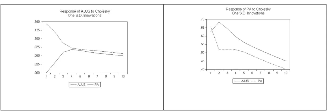
The response-impulse functions showed in Figure 1 were estimated in first differences [16], indicating the effects of short-term TA and PH variables.
The shocks estimated in this model could be due to events such as change of raw materials and/or machinery, change in the set point in the production batch, shift time, failures in the supply of electricity, defective heating lamps in the oven or burned, and/or even a sudden change of room temperature. These changes are captured by the response-impulse and transmitted to other system variables that may influence the quality characteristics in the final product.
Figure 1 shows that the impulse has different behaviors regarding the innovations. When an increase in the oven temperature, i.e., a high percentage of heating is observed, it is necessary to reduce the degree of heating inside the oven. Thus, the knob must be set as a way to control the heating in the oven. On the other hand, when there is a decrease in the percentage of heating, it is necessary to increase the degree of temperature inside the oven. Thus, the knob must be adjusted as a way to release the heating temperature in the oven.
Fig. 1. Impulse-response functions of the variable heating rate and oven adjustment
According to [21], if there is a relationship between two variables that can be manipulated to achieve a state of control and they are measured at equidistant interval of time, a change in the control variable may have its effect dissipated by several subsequent time periods. Thus, it is important to find the time or delay that this action may take to be accomplished. Therefore, it is important to find the period in which the equilibrium occurs. The bottle made by PTR preform molding reaches temperature equilibrium in the oven only four hours after a shock occurs,
i.e., a change in the control variable may affect the process up to 4 h.
The origin of error correction model is from economy and therefore economic reasons have always been sought in order to justify the long-run equilibrium. In the quality control area, other reasons try to justify the variable behavior, i.e., the feature and specification of the heating oven and the kind of material that will be heated.
Given the necessary time that the oven takes to achieve the desired heat level, one should take into account its physical properties, as well as the differences between the nominal value of heat released or restricted in the oven and the achieved value. Not always 100% is effective because during this process losses occur through heat exchange system itself with the environment, with the inlet temperature of the preforms and other factors. However, it is known and we should be aware that the quality of 2-liter bottles depends on the maintenance of temperature at levels established by the specifications of the product, otherwise the production of defective items may occur.
Table 5 shows the Granger Causality test performed to verify the direction of causality between the two variables.
Table 5. Test of Granger causality between TA and PH variables of the molding oven temperature
Null hypothesis Observations F-Statistic Probability
PA does not Granger Cause AJ 200 14.4176 1.4E-06
AJ does not Granger Cause PA 200 2.42551 0.09110
A unidirectional causality transmission was observed during the process. The PH causes the temperature adjustment in the oven, being the responsible for the changes that may occur. These changes are introduced to maintain the process stable and to follow the specifications to be produced in each lot. As the system takes 4 h to reach equilibrium, it is necessary to be very careful, during this period, not to over-manipulate the controls in order to quickly achieve the specifications and make the system completely out of control.
Since the monthly production of the company is estimated at 1.6 million units of 2 liter plastic bottles per month, the company should have an intense care to avoid waste.
5. CONCLUSIONS
The application of the error correction model allowed identifying the behavior of the variables responsible for the quality characteristic of 2-liter bottles made from polyethylene terephthalate resin molding in the stage of oven. Moreover, it provided the direction of causality and time required for the oven to reach the required equilibrium for its use, and the low level of defective product.
The instability of the oven may cause molding defects in bottles, which do not allow using them in subsequent stages of the production process, incurring in extra costs of production.
Besides presenting a methodology capable of determining the estimated time to achieve the equilibrium in the system, it is important to know which variable to manipulate and how long it takes to reach the equilibrium after introducing a change or suffer an external shock. The methodology of the error correction model provided a new tool to help monitor and understand the variables responsible to maintain the process under control.
For further studies we suggest the joint application of SPC and EPC methodologies [19], so that we can achieve stability of the system by adjusting the feedback control as well as a monitoring process by means of SPC after implements and adjustment in the process.
364 | www.ijar.lit.az
ACKNOWLEDGMENTS
We thank the financial support of CAPES – Process - BEX 1784/09-9 - CAPES Foundation, Ministry of Education of Brazil - Brasilia The authors also thank the financial support provided by Fundação para a Ciência e Tecnologia (FCT) under the grants # PTDC/GES/73418/2006 and # PTDC/GES/70529/2006.
REFERENCES
1. Souza, A. M.; Samohyl, R. W.; Malavé, C. O, Multivariate feedback control: an application in a productive process, Computers & Industrial Engineering, v. 46, p. 837-850, 2004.
2. Box, G.E.P. and Luceño, A, Discrete proportional-integral adjustment and statistical process control, Journal of Quality Technology, July v.29, n. 3, 1997.
3. Bentes, S.R.; Menezes, R.; Mendes, D. A., Long memory and volatility clustering: is the empirical evidence cossistent across stock markets?, Physica A. v. 387, issue 15, june 2008.
4. Clausius, R, On the Motive Power of Heat, and on the Laws which can be deduced from it for the Theory of Heat, Poggendorff's Annalen der Physick, LXXIX (Dover Reprint), 1850.
5. Bueno, R. L. S, Econometria de séries temporais. São Paulo: Cengage Learning, 2008.
6. Portugal, S. M, Um modelo de correção de erros para a demanda por importações brasileiras. Pesq. Plan. Econ. V. 22, n. 3; p. 501-540; dez. 1992.
7. Gujarati, D. N. Econometria básica. São Paulo: Makron Books, 2000.
8. Bentes, S.R., R. Menezes e Mendes. D.A, Long memory and volatility clustering: Is the empirical evidence consistent across stock markets? Physica A 387, 3826-3830, 2008.
9. Enders, W, Applied econometric time series, New York: John Wiley and Sons, Inc., 1995. 10. Maddala, G. S, Introduction to econometrics, 2.ed. New Jersey: Prentice Hall, 1992.
11. Morettin, P. A, Econometria financeira – um curso em séries temporais. São Paulo: Blucher, 2008. 12. Alexander, C, Modelos de mercados: um guia para a análise de informações Finaceiras (Tradução
José Carlos de Souza Santos), São Paulo: Bolsa de Mercadorias & Futuros, 2005.
13. Baptista, A. J. M. S. e Coelho A. B, Previsão de inflação em Cabo Verde por meio de vetores autoregressivos, Anais do XLII Congresso da Sociedade Brasileira de Economia e Sociologia Rural, Dinâmicas Setoriais e Desenvolvimento Regional. Sociedade Brasileira de Economia e Sociologia Rural, Cuiabá - MT, 25 a 28 de julho de 2004.
14. Johansen, S, Statistical analysis of cointegration vectors, Journal of Economic Dynamics and Control. V. 12, 231 – 254, 1988.
15. Johansen, S., Identify restrictions of linear equations with applications to simultaneous equations and cointegration, Journal of Econometrics, V.69, 111-132, 1995.
16. Doornick, J.A., Hendry, D.F, Nielsen, B., Inferences in cointegrating models: UK M1 revisited, Journal of Economic Survey. Vol. 2, n.5, 1998.
17. Menezes, R, Market integration and the globalization of stock markets: Evidence from five countries, Working Paper, ISCTE – IUL, 2009.
18. Johansen, S.; Juselius, K, Maximum likelihood estimation and inference on cointegration: with applications to the demand for money. Oxford Bulletin of Economics and Statistics, v.52, p.169-219, 1990.
19. Granger, C.W.J, Investigating causal relations by econometric models and cross-spectral models, Econometrica 34, 541-51. 1969.
20. Del Castillo, E, Statistical control adjustment for quality control, Canadá: John Wiley & Sons, Inc., 2002.
21. Bender Filho, R. e Alvim, A. M, Análise da transmissão de preços da carne bovina entre os países do MERCOSUL e Estados Unidos, Anais da Sociedade Brasileira de Economia, Administração e Sociologia Rural, Rio Branco – Acre, 20 a 23 de julho de 2008.