Mahsa Kiazadeh
Assessing the Existence of Visual Clues
of Human Ovulation
Universidade do Algarve
2019
Mahsa Kiazadeh
Assessing the Existence of Visual Clues
of Human Ovulation
Master Thesis in Informatics Engineering
Work done under the supervision of:
Prof. Hamid Reza Shahbazkia
Prof. Gabriela Gonçalves
Universidade do Algarve
2019
Statement of Originality
Assessing the Existence of Visual Clues of Human Ovulation
(Master Thesis in Informatics Engineering)
Statement of authorship: The work presented in this thesis is, to the best of my knowledge and belief, original, except as acknowledged in the text. The material has not been submitted, either in whole or in part, for a degree at this or any other university.
Candidate: ——————————— (Mahsa Kiazadeh)
Copyright© Mahsa Kiazadeh. A Universidade do Algarve tem o direito, perpetuo e sem limites geográficos, de arquivar e publicitar este trabalho através de exemplares impressos reproduzidos em papel ou de forma digital, ou por qualquer outro meio conhecido ou que venha a ser inventado, de o divulgar através de repositórios científicos e de admitir a sua copia e distribuição com objetivos educacionais ou de investigação, não comerciais, desde que seja dado credito ao autor e editor.
Abstract
Is the concealed human ovulation a myth? The author of this work tries to answer the above question by using a medium-size database of facial images specially created and tagged. Analyzing possible facial modifications during the mensal period is a formal tool to assess the veracity about the concealed ovulation. In normal view, the human ovulation remains concealed. In other words, there is no visible external sign of the mensal period in humans. These external signs are very much visible in many animals such as baboons, dogs or elephants. Some are visual (baboons) and others are biochemical (dogs). Insects use pheromones and other animals can use sounds to inform the partners of their fertility period.
The objective is not just to study the visual female ovulation signs but also to understand and explain automatic image processing methods which could be used to extract precise landmarks from the facial pictures. This could later be applied to the studies about the fluctuant asymmetry. The field of fluctuant asymmetry is a growing field in evolutionary biology but cannot be easily developed because of the necessary time to manually extract the landmarks.
In this work we have tried to see if any perceptible sign is present in human face during the ovulation and how we can detect formal changes, if any, in face appearance during the mensal period.
We have taken photography from 50 girls for 32 days. Each day we took many photos of each girl. At the end we chose a set of 30 photos per girl representing the whole mensal cycle. From these photos 600 were chosen to be manually tagged for verification issues. The photos were organized in a rating software to allow human raters to watch and choose the two best looking pictures for each girl. These results were then checked to highlight the relation between chosen photos and ovulation period in the cycle. Results were indicating that in fact there are some clues in the face of human which could eventually give a hint about their ovulation.
Later, different automatic landmark detection methods were applied to the pictures to highlight possible modifications in the face during the period. Although the precision of the tested methods, are far from being perfect, the comparison of these measurements to the state of art indexes of beauty shows a slight modification of the face towards a prettier face during the ovulation.
The automatic methods tested were Active Appearance Model (AAM), the neural deep learning and the regression trees. It was observed that for this kind of applications the best method was the regression trees.
Future work has to be conducted to firmly confirm these data, number of human raters should be augmented, and a proper learning data base should be developed to allow a learning process specific to this problematic. We also think that low level image processing will be necessary to achieve the final precision which could reveal more details of possible changes in human faces.
Keywords: Image processing, Facial landmark extraction, Learning based methods, Human ovulation, Fluctuant asymmetry.
Resumo
A ovulação no ser humano é, em geral, considerada “oculta”, ou seja, sem sinais exteriores. Mas a ovulação ou o período mensal é uma mudança hormonal extremamente importante que se repete em cada ciclo. Acreditar que esta mudança hormonal não tem nenhum sinal visível parece simplista. Estes sinais externos são muito visíveis em animais, como babuínos, cães ou elefantes. Alguns são visuais (babuínos) e outros são bioquímicos (cães). Insetos usam feromonas e outros animais podem usar sons para informar os parceiros do seu período de fertilidade. O ser humano tem vindo a esconder ou pelo menos camuflar sinais desses durante a evolução. As razoes para esconder ou camuflar a ovulação no ser humano não são claros e não serão discutidos nesta dissertação.
Na primeira parte deste trabalho, a autora deste trabalho, depois de criar um base de dados de tamanho médio de imagens faciais e anotar as fotografias vai verificar se sinais de ovulação podem ser detetados por outros pessoas. Ou seja, se modificações que ‘as priori’ são invisíveis podem ser percebidas de maneira inconsciente pelo observador. Na segunda parte, a autora vai analisar as eventuais modificações faciais durante o período, de uma maneira formal, utilizando medidas faciais. Métodos automáticos de analise de imagem aplicados permitem obter os dados necessários.
Uma base de dados de imagens para efetuar este trabalho foi criado de raiz, uma vez que nenhuma base de dados existia na literatura. 50 raparigas aceitaram de participar na criação do base de dados. Durante 32 dias e diariamente, cada rapariga foi fotografada. Em cada sessão foi tirada várias fotos. As fotos foram depois apuradas para deixar só 30 fotos ao máximo, para cada rapariga. 600 fotos foram depois escolhidas para serem manualmente anotadas. Essas 600 fotos anotadas, definam a base de dados de verificação. Assim as medidas obtidas automaticamente podem ser verificadas comparando com a base de 600 fotos anotadas.
O objetivo deste trabalho não é apenas estudar os sinais visuais da ovulação feminina, mas também testar e explicar métodos de processamento automático de imagens que poderiam ser usados para extrair pontos de interesse, das imagens faciais. A automatização de extração dos pontos de interesse poderia mais tarde ser aplicado aos estudos sobre a assimetria flutuante. O campo da assimetria flutuante é um campo crescente na biologia evolucionária, mas não pode
ser desenvolvido facilmente. O tempo necessário para extrair referencias e pontos de interesse é proibitivo. Por além disso, estudos de assimetria flutuante, muitas vezes, baseado numa só fotografia pode vier a ser invalido, se modificações faciais temporárias existirem. Modificações temporárias, tipo durante o período mensal, revela que estudos fenotípicos baseados numa só fotografia não pode constituir uma base viável para estabelecer ligas genótipo-fenótipo.
Para tentar ver se algum sinal percetível está presente no rosto humano durante a ovulação, as fotos foram organizadas num software de presentação para permitir o observador humano escolher duas fotos (as mais atraentes) de cada rapariga. Estes resultados foram então analisados para destacar a relação entre as fotos escolhidas e o período de ovulação no ciclo mensal. Os resultados sugeriam que, de facto, existem algumas indicações no rosto que poderiam eventualmente dar informações sobre o período de ovulação. Os observadores escolheram como mais atraente de cada rapariga, aquelas que tinham sido tiradas nos dias imediatos antes ou depois da ovulação. Ou seja, foi claramente estabelecido que a mesma rapariga parecia mais atraente durante os dias próximos da data da ovulação. O software também permite recolher dados sobre o observador para analise posterior de comportamento dos observadores perante as fotografias. Os dados dos observadores podem dar indicações sobre as razoes da ovulação escondida que foi desenvolvida durante a evolução.
A seguir, diferentes métodos automáticos de deteção de pontos de interesse foram aplicados às imagens para detetar o tipo de modificações no rosto durante o período. A precisão dos métodos testados, apesar de não ser perfeita, permite observar algumas relações entre as modificações e os índices de atratividade.
Os métodos automáticos testados foram Active Appearance Model (AAM), Convolutional Neural Networks (CNN) e árvores de regressão (Dlib-Rt). AAM e CNN foram implementados em Python utilizando o modulo Keras library. Dlib-Rt foi implementado em C++ utilizando OpenCv. Os métodos utilizados, estão todos baseados em aprendizagem e sacrificam a precisão. Comparando os resultados dos métodos automáticos com os resultados manualmente obtidos, indicaram que os métodos baseados em aprendizagem podem não ter a precisão necessária para estudos em simetria flutuante ou para estudos de modificação faciais finas. Apesar de falta de precisão, observou-se que, para este tipo de aplicação, o melhor método (entre os testados) foi as árvores de regressão.
Os dados e medidas obtidas, constituíram uma base de dados com a data de período, medidas faciais, dados sociais e dados de atratividade que poderem ser utilizados para trabalhos posteriores.
O trabalho futuro tem de ser conduzido para confirmar firmemente estes dados, o número de avaliadores humanos deve ser aumentado, e uma base de dados de aprendizagem adequada deve ser desenvolvida para permitir a definição de um processo de aprendizagem específico para esta problemática. Também foi observado que o processamento de imagens de baixo nível será necessário para alcançar a precisão final que poderia revelar detalhes finos de mudanças em rostos humanos. Transcrever os dados e medidas para o índice de atratividade e aplicar métodos de data-mining pode revelar exatamente quais são as modificações implicadas durante o período mensal. A autora também prevê a utilização de uma câmara fotográfica tipo true-depth permite obter os dados de profundidade e volumo que podem afinar os estudos. Os dados de pigmentação da pele e textura da mesma também devem ser considerados para obter e observar todos tipos de modificação facial durante o período mensal.
Os dados também devem separar raparigas com métodos químicos de contraceção, uma vez que estes métodos podem interferir com os níveis hormonais e introduzir erros de apreciação.
Por fim o mesmo estudo poderia ser efetuado nos homens, uma vez que homens não sofrem de mudanças hormonais, a aparição de qualquer modificação facial repetível pode indicar existência de fatos camuflados.
Termos chave: Processamento de imagem, Extração do marco facial, Métodos baseados na aprendizagem, Ovulação humana, Assimetria flutuante.
Table of Contents
Statement of Originality II Abstract III Resumo V Motivation 1 Objective 2 Methodology 3Fluctuant Asymmetry overview 3
Concealed ovulation 6
Facial analysis and Landmark extraction 8
Expression analysis 10
Component based Deformable Mode 11
Cascade Deformable Shape model 12
Constrained Local Neural Field model (CLNF) 13
Deep Convolutional Network Cascade 13
Coarse-to-fine Convolutional Network Cascade 14
Explicit Shape Regression 15
Constrained local models (CLM) 15
Parameterized Kernel Principal Component Analysis (PKPCA) 16
Multiple Kernel Learning 16
Semi - Supervised learning 17
Bayesian Approach 18
Multi View 19
Combinatorial Search and Shape Regression 20
Tree-structured models 20
Supervised Descent Method 21
Introduction 22
Data collection 22
Human rating 22
Implementations 25
Active appearance models 25
Convolutional neural networks and deep learning 28
Architecture Overview 28
Learning process 31
Data preparation 34
Training 35
Regression trees using the Dlib library 37
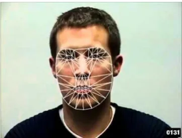
Ground truth Hand marking of the data set 40
Rating results 42
Automatic landmark extraction results 49
The AAM results 50
The CNN results 51
The Dlib results 53
Comparing the results between methods 56
Introduction
Motivation
A living organism develops and creates a particular form following its genetic program. The type of the genetic program is of course different in each individual, not only between species but also within the species. This particular program is called the genotype. During the development of the fetus, the pre-programmed genetic path manages the form that the individual will have in its final form and this form is called the phenotype.
Following this definition and the reality, one can suppose that each phenotype represents a special genotype and therefore by analyzing only the forms of individual, genetic information and some clues about the genotype can be retrieved.
Going a bit deeper in this issue and following the evolutionary biology about the fetus and pre-puberty development, this genotype needs to defend the organism development against all environmental stress and to execute the program the best possible. For example, development of a pair of organs which normally have to be symmetrical and be distributed identically on either side of the body should be exactly the same. These organs such as eyes, ears, hands, legs, etc. appear in a symmetrical position. The capacity of the genotype to create this symmetry in the final form of the individuals is believed by biologists to be a sign of quality. In other word, a better symmetry means a better genotype. It is therefore normal that a lot of work and studies concentrate on understanding the links between this symmetry in the phenotype and the genotype. Possible links between facial asymmetry and predisposition to some genetic alterations or diseases is an important issue of such studies. A very large interval of research is possible. Such as sexual attraction passing by genetic illness, or mental disorder possible links with visual facial clues, etc.
Nevertheless, a bottleneck of this field of study is the time necessary for the researcher to pinpoint the landmarks on a face and to calculate manually the possible ratios and symmetry on each single picture. This time-consuming process of manual calculation and analysis have not yet allowed large scale studies in this domain and all possible studies done so far remain on a small number of cases (mostly less than 100). It is therefore obvious that an automatic tool for
extraction of facial landmarks and precise processing of visual clues is an absolute necessity to solve the main bottleneck in this field of study. If this tool is developed, then a full-scale analysis becomes possible and most of the theories in this field can either be confirmed or rejected in a robust manner.
Now what this facial asymmetry has to do with the topic of this work? Well, the problem of manual analysis is only one aspect that prohibits the verification of different theories on this field. Another point of discussion between some communities lays on the fact that most evolutionary biologists consider that the final form of an individual is achieved after the puberty and this form does not change in a short period of time. Therefore, most of the studies over the face asymmetry are done by working only over one picture of the individual. The proponents of this work, nevertheless, think that this is not the case. Studying one picture of an individual taken in a particular moment can introduce a lot of bias into the final study of the facial signs and their links to other abnormalities.
Objective
As everyone knows, on some days people look better and, on some days, they look worse. Taking one picture of this individual for analyzing its genotype where we all know that the study is based over very little differences seems a bit unexplainable. This single picture is not really the best way to study possible life term links between phenotype and genotype. To demonstrate and prove that individual faces can show minor differences even in short term, the proponents of this study have searched a special case of physiological changes in human body in short terms that may affect the facial form.
The best and straight forward case in human of a deep physiological change in a short period of time is the mensal cycle in women. This fix periodical physiological change modifies deeply the biochemical composition in the body by modification of different levels of hormones. The fact of the periodicity of these phenomena is also a positive point because it allows the total repeatability of the study whenever necessary. If a facial modification during the mensal period is proved and formally calculated, then it is clear that most studies over links between facial symmetry and genotype abnormalities are to be repeated as they are only based on single photography.
This in the beginning was the main motivation of this study. Nevertheless, when the study was initiated, and the idea clarified a much bigger domain is to be explored. This fact has now made this study a full possible multidisciplinary research subject which can have repercussions in basic beliefs over human behavior and well-established issues such as concealed ovulation. If it is proved that external signs of ovulation do exist in each mensal cycle, and then many other questions will be open such as are they for all? Who detects best? Is it in every cycle or only in some?
Methodology
To be able to manage this study in a statically correct manner we need of course to solve the manual analysis bottleneck and develop an automatic manner of measuring facial landmarks. The extraction of the measurements automatically will allow a swift path towards large scale study and eliminate all bias. The objective of the proposed work is to be divided into two main streams:
• To develop a simple program to allow the ratters to choose in a short time best pictures of each woman during the mensal cycle. This will allow us to access the existence of possible visual points which could appear during the hormonal modification in the body.
• To use image processing techniques, mainly active appearance models to understand exactly what these changes are in an automatic manner. The mathematical model of the faces can then be studied to explain why in this short period of time the same individual looks more attractive.
In the following parts of this report a background over fluctuant asymmetry and concealed ovulation as well as facial automatic analysis will be exposed.
Background
Fluctuating asymmetry is a particular form of biological asymmetry, characterized by small random deviations from perfect symmetry. The fundamental basis for the study of fluctuating asymmetry is an a priori expectation that symmetry is the ideal state of bilaterally paired traits.
Fluctuating asymmetry measures deviations from the ideal state of symmetry and is therefore thought to reflect the level of genetic and environmental stress experienced by individuals or populations during development. It has attracted a great deal of attention because bilaterally symmetrical traits are extremely common in nature and because the measurement of fluctuating asymmetry appears to represent a relatively simple method of assessing biologically important stress at the individual and population levels.
Asymmetry of an individual is measured as the right minus the left value of the bilaterally paired trait. By studying the distribution of these asymmetries at the population level, we can distinguish between three types of biological asymmetry: fluctuating asymmetry, directional asymmetry, and symmetry. Fluctuating asymmetry is characterized by small random deviations from perfect bilateral symmetry. These small random deviations result in a normal or leptokurtic distribution of asymmetry around a mean of zero. Directional asymmetry is characterized by a symmetry distribution that is not centered around zero but is biased significantly, towards larger traits either on the left or the right side.
Anti-symmetry is characterized by being centered around a mean of zero; however, symmetric individuals are rarer than those seen in fluctuating asymmetry distributions, such that the distribution is platykurtic or, in the extreme, bimodal. Directional symmetry and antisymmetric are developmentally controlled and therefore likely to have adaptive significance. Fluctuating asymmetry, on the other hand, is not likely to be adaptive as symmetry is expected to be the ideal state [1][2] although subtracting the measurement of the right side of a trait from that of the left side forms the basis of the analysis, accurately quantifying fluctuating asymmetry is not simple.
The measurement of fluctuating asymmetry is complicated by the fact that its magnitude and distribution are the same as the magnitude and distribution of measurement error. Therefore, in order to establish that real differences in symmetry rather than just measurement error are being reported, it is imperative to establish that the measures of fluctuating asymmetry
explain a statistically significant proportion of the observed total variance between the sides. To achieve this, it is necessary to make repeated measures of the left and right sides of the trait. The repeated measures need to be made on the same subjects in ignorance of the initial measure, with the same equipment and under the same laboratory or field circumstances as those of the main data. Furthermore, to eliminate observer bias, ideally all measurements should be made in ignorance of the measurement recorded for the side’s pair.
For analysis of a potential fluctuating asymmetry data set, certain criteria must be met: the measurements must represent actual deviations from symmetry and not measurement error, and the distribution of fluctuating asymmetry must conform to that expected for it, rather than for directional asymmetry or anti symmetry. Various procedures have been recommended for this stage of the analysis, the most widely used being a mixed model analysis of variance (ANOVA), which will determine whether fluctuating asymmetry is significantly different from measurement error, and whether the asymmetry distribution has a mean of zero [1]. The mixed model ANOVA does not reveal significant departures in the fluctuating asymmetry distribution towards platy kurtosis, characteristic of anti-symmetry, and therefore the asymmetry distribution should also be described statistically in terms of its kurtosis and assessed visually.
Fluctuating Asymmetry trait, data analysis should proceed by testing first for the relation between trait size and fluctuating asymmetry. If there is a relationship, this needs to be accounted for, and methods exist for controlling for size dependence [1]. Data can be analyzed between groups, treatments or populations by using methods for comparing trait variances. Relationships between individual fluctuating asymmetry and continuous variables such as fitness measures need to be conducted on absolute fluctuating asymmetry values, sometimes called ‘unsigned fluctuating asymmetry’. Caution should be exercised when analyzing unsigned fluctuating asymmetry, as it has a half-normal distribution, which violates the assumptions of most parametric statistics. A more accurate assessment of developmental stability can be obtained by pooling the fluctuating asymmetry measures of several traits per individual. However, as different traits may have different selection pressures on their symmetry, the traits that are being pooled need to be chosen carefully. It is a common observation that there is at best a very weak relationship between fluctuating asymmetries measured from two different traits for the same individuals.
Concealed ovulation
Concealed ovulation or hidden estrus in a species is the lack of any perceptible change in an adult female (for instance, a change in appearance or scent) when she is "in heat" and near ovulation. Some examples of such changes are swelling and redness of the genitalia in baboons and bonobos Pan paniscus, and pheromone release in the feline family. In contrast, the females of humans and a few other species [3] have few external signs of fecundity, making it difficult for the male to consciously deduce, by means of external signs only, whether or not a female is near ovulation.
While women can be taught to recognize their own level of fertility (fertility awareness), whether men can detect fertility in women is highly debated. Several small studies have found that fertile women (compared to women in infertile portions of the menstrual cycle or using hormonal contraception) appear more attractive to men [4][5]. It has also been suggested that a woman's voice may become more attractive to men during this time [6]. Two small studies of monogamous human couples found that women-initiated sex significantly more frequently when fertile, but male-initiated sex occurred at a constant rate, without regard to the woman's phase of menstrual cycle [7]. It may be that a woman's awareness of men's courtship signals [8] increases during her highly fertile phase due to an enhanced olfactory awareness of chemicals specifically found in men's body odor [9][10] Analyses of data provided by the post-1998 U.S. Demographic and Health Surveys found no variation in the occurrence of coitus in the menstrual phases (except during menstruation itself) [11]. This is contrary to other studies, which have found female sexual desire and extra-pair copulations ("EPC's") to increase during the mid-follicular to ovulatory phases (that is, the highly fertile phase) [12]. These findings of differences in woman-initiated versus man-initiated sex are likely caused by the woman’s subconscious awareness of her ovulation cycle (because of hormone changes causing her to feel increased sexual desire), contrasting with the man’s inability to detect ovulation because of its being “hidden”.
In 2008, researchers announced the discovery in human semen of hormones usually found in ovulating women. They theorized that follicle stimulating hormone, luteinizing hormone, and estradiol may encourage ovulation in women exposed to semen. These hormones are not found in the semen of chimpanzees, suggesting this phenomenon may be a human male
counterstrategy to concealed ovulation in human females. Other researchers are skeptical that the low levels of hormones found in semen could have any effect on ovulation [13]. One group of authors has theorized that concealed ovulation and menstruation were key factors in the development of symbolic culture in early human society [14][15].
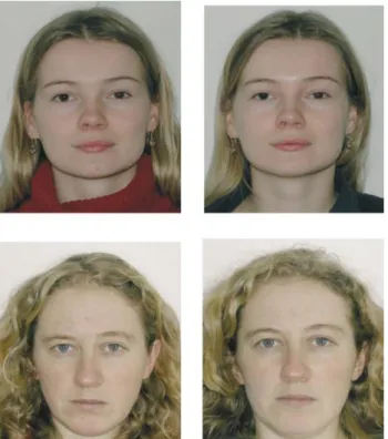
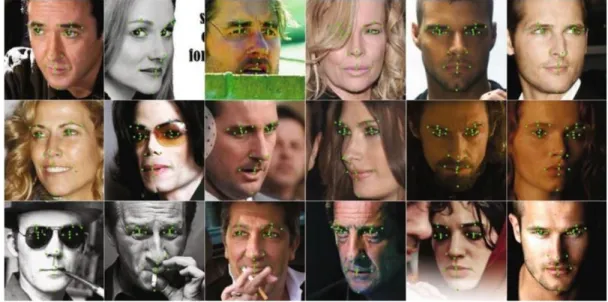
Figure 2.1: Image pairs of two women as examples of stimuli used: (a) is from Prague; and (b) is from Newcastle. One image in each pair was taken during the follicular phase (i) and one in the luteal phase (ii) of the cycle (in both cases, days 12 and 19, respectively
Human differs from other mammalians in their sexual behavior [1]. One of the most intriguing fact in this behavior is the concealed ovulation (The ovulation without any external visible signs). Many theories over the how and why of human move out from an advertised oestrus cycle to a concealed menstruation cycle has been developed [2] and for years it was conventionally accepted that the oestrus was either lost or completely concealed. Nevertheless, the idea of a completely hidden and sign-less period of fertility sounds contradictory to normal rules of reproductively and mate selection. Some recent studies using fine-tuned phenotype measurements have revealed that some signs appear at the fertile point of the cycle to make the female more attractive to male. Studies over body scent, voice frequency. Soft tissue symmetry, body ratio, creativity and fluidity in speech and facial attractiveness were assessed and studied as possible modifications that alerts a male over the fecundity of the female. Some other studies
over the number of tips gained by lap dancers in different period of their mensal cycle shows that the dancers earned much more during the oestrus or just before ovulation.
As one can see through these studies that hearing, smell and sight could all be used to receive fertility signs, but the human society defines attractiveness solely by means of sight. Therefore, if signs of oestrus do exist between human, they should mostly be present in visual cues. In this paper we focus on facial attractiveness during the cycle. The previous study on the subject have revealed possible signs but in a very limited proportion, Roberts & al used only 2 photos of women one in follicular phase and one in lethal phase to distinguish between possible visual cues. The results obtained by Roberts & al were just a bit over the random of 0.5 expected. The authors recognize also that their study could only suggest a fluctuant facial attractiveness during the mensal cycle.
Facial analysis and Landmark extraction
A facial biometric system is a computer application for automatically identifying or checking a person from a numeric image or from a video frame from a video source. One approach to do so, is comparing selected facial features from the image and a facial database. It is typically used in security systems and can be compared to other biometrics such as fingerprint or iris recognition systems. Some facial recognition algorithms identify facial features by extracting landmarks, or features, from an image of the subject's face. For example, an algorithm may analyze the relative position, size, and/or shape of the eyes, nose, cheekbones, and jaw. These features are then used to search for other images with matching features.
Other algorithms after normalizing a data base of images keep only the data necessary for the process of recognition and save them. A probe image is then compared with the face data. One of the earliest successful systems [18] is based on template matching techniques applied to a set of salient facial features, providing a sort of compressed face representation. Recognition algorithms can be divided into two main approaches, geometric, which look at distinguishing features, or photometric, which is a statistical approach that transforms an image into values and compares the values with templates. Popular recognition algorithms include Principal Component Analysis using eigenfaces, Linear Discriminate Analysis, Elastic Bunch Graph Matching using the Fisher-face algorithm, the Hidden Markov model, the Multilinear Subspace
Learning using tensor representation, and the neuronal motivated dynamic link matching.
We will be referring often in this document to the landmarks. A landmark is a recognizable natural or man-made feature that stands out from its near environment and is often visible from long distances. Facial landmarks are defined as key-points on the face with subsequent impact on the target task, like animation, face recognition, gaze detection, face tracking, expression recognition, gesture understanding etc. Facial landmarks are a prominent feature that can play a discriminative role or can serve as anchor points on a face graph. Facial landmarks such as the nose tip, eyes corners, chin, mouth corners, nostril corners, eyebrow arcs, ear lobes, are the common choices. For ease of analysis most landmark detection algorithm prefers an entire facial semantic region, such as the whole region of a mouth, the region of the nose, eyes, eyebrows, cheek or chin. The facial landmarks are classified in two groups, primary and secondary, or fiducial and ancillary. This distinction is based on reliability of image features detection techniques. For example, the corners of the mouth, of the eyes, the nose tips and eyebrows can be detected relatively easily by using low level image features, e.g. SIFT, HOG. The directly detected landmarks are referred as fiducial. The fiducial group of landmarks play a more prominent role in facial identity and face tracking. The search for secondary landmarks is guided by primary landmarks. The secondary landmarks are chin, cheek contours, eyebrow and lips midpoints, non-extremity points, nostrils. It takes more prominent role in facial expression [19].
Despite the conceptual simplicity of facial landmarks detection, in computer vision there are some challenges. The emerging applications like surveillance system, gesture recognition requires that landmark localization algorithms should run in real time parallel with the computational power of an embedded system, such as intelligent cameras. Such type of application requires a more robust algorithms against a confounding factor such as illumination effects, expression and out of plane pose. There are four main challenges in localizing facial landmarks [19]:
• Variability: Landmark appearances differ due to extrinsic factors such as partial occlusion, pose, illumination, camera resolution and expression, also due to intrinsic factors such as face variability between individuals. Facial landmarks can sometimes be only partially observed due to hand movements or self-occlusion due
to extensive head rotations or occlusions of hair. Also, facial landmark detections are difficult because of illumination artifacts and facial expressions. A facial landmark localization algorithm that delivers the target points in a time in an efficient manner and works well across all intrinsic variations of faces has not yet been feasible.
• Accuracy and number of landmarks require: Based on the intended application the number of landmarks and its accuracy varies. For example, in face recognition or in face detection tasks, primary landmarks like two mouth corner, four eyes corner and nose tips may be adequate. On the other hand, higher level tasks face animation or facial expression understanding require greater number of landmarks e.g. from 20-30 to 60 - 80 with higher accuracy. Fiducial landmarks are needed to be determined with more accuracy because they often guide the search of secondary landmarks.
• Lack of globally accepted and error free dataset: Most of the dataset provides annotations with different markups and accuracy of their fiducial point is questionable. The accuracy of landmark localization algorithm is largely depending on the data set used for training. Each algorithm uses different dataset to train and evaluate the performance, so it is difficult to compare algorithms.
• Acquisition conditions: Acquisition conditions, such as resolution, background clutter, and illumination can affect the landmark localization performance. The landmark localizers trained in one database have usually inferior performance when tested on another database. It is to mention that these challenges, are general case study challenges. In the particular case in scope of the present work we will not be dealing with variability or acquisition conditions because they were fixed in lab conditions and the external factors were kept as equal as possible between images. Nevertheless, we were not able to keep the exact lighting or contrast conditions.
Expression analysis
intention, personality, and psychopathology of a person [20], it plays a communicative role in interpersonal relations. Facial expressions, and other gestures, convey non-verbal communication cues in face-to-face interactions. These cues may also complement speech by helping the listener to elicit the intended meaning of spoken words. As cited in [21], Mehrabian reported that facial expressions have a considerable effect on a listening interlocutor, the facial expression of a speaker accounts for about 55 percent of the effect, 38 percent of the latter is conveyed by voice intonation and 7 percent by the spoken words.
As a consequence of the information that they carry, facial expressions can play an important role wherever humans interact with machines. Automatic recognition of facial expressions may act as a component of natural human- machine interfaces [22] (some variants of which are called perceptual interfaces [23] or conversational [24] interfaces). Such interfaces would enable the automated provision of services that require a good appreciation of the emotional state of the service user, as would be the case in transactions that involve negotiation, for example. Some robots can also benefit from the ability to recognize expressions [25].
Automated analysis of facial expressions for behavioral science or medicine is another possible application domain [26][27]. From the viewpoint of automatic recognition, a facial expression can be considered to consist of deformations [28] of facial components and their spatial relations, or changes in the pigmentation of the face. Research into automatic recognition of facial expressions addresses the problems surrounding the representation and categorization of static or dynamic characteristics of these deformations or face pigmentation. Further details on the problem space for facial expression analysis are given in [29]. We will continue with a survey of some of the recent landmark localization techniques [19]
Literature survey of localization techniques
Component based Deformable Mode
Component based deformable model presented for generalized face alignment at 2007 [30], they used a novel bi-stage statistical framework to account for both local and global shape characteristics. It uses separate Gaussian models for shape components instead of using
statistical analysis on the entire shape which preserve more detailed local shape deformations. Each model of components used the Markov Network for search strategy. They used Gaussian Process Latent Variable Model to give control of full range shape variations, hence it makes out better description of the nonlinear interrelationships over shape components. This approach allows the system to preserve the full range of low frequency shape variations, and also the high frequency local deformations caused by exaggerated expression.
Figure 3.1: Output of component based deformable model – (Database: YALE FACE DATABASE B, Key point detected: 79 Image / video: Images only)
Cascade Deformable Shape model
Xiang, et al, [31] presents a two-stage cascaded deformable shape model to effectively and efficiently localize facial landmarks with large head pose variations. For face detection, they proposed a group sparse learning method to automatically select the most salient facial landmarks. 3D face shape model detects pose free facial landmark initialization. The deformation executes in two stages, the first step uses mean-shift local search with constrained local model to rapidly approach the global optimum. Second step uses component-wise active contours to discriminatively refine the subtle shape variation. It improves performance over CLM and multi-ASM in face landmark detection and tracking.
Figure 3.2: Output of cascade deformable shape model – (Database: MultiPIE, AR, LFPW,LFW and AFW ,Talking Face Video, Key point detected: 65, Image / video: Images and video both)
Constrained Local Neural Field model (CLNF)
Baltrusaitis and et al, [32] presented the Constrained Local Neural Field model for facial landmark detection. This model uses probabilistic patch expert (landmark detector) that learn non-linear and spatial relationships between the input pixels and the probability of a landmark being aligned and Non-uniform Regularized Landmark Mean-Shift (NRLM) optimization technique, which takes the account the reliabilities of each patch expert leading to better accuracy.
Figure 3.3:Output of constrained local neural field model – (Database: LFPW and Helen, Key point detected: 65, Image / video: Images only)
Deep Convolutional Network Cascade
Yi Sun [33] presented three level deep convolutional networks cascade model. The output of multiple networks at each level is fused to give robust and accurate estimation. At first level, convolutional networks extracts high level features over whole face region. It has two advantages first, the texture context information over the entire face is utilized to locate key point. Second, the network is trained to predict all the key-points simultaneously, geometric
constraints among key-points are encoded. Therefore, method avoids local minimum caused by ambiguity and data corruption. In next two level the initially predicted key-points are finely-tune to achieve high accuracy. This method is not good for locating facial landmarks in large number.
Figure 3.4: Output of deep convolutional network cascade – (Database: LFW,LFPW and BioID Key point
Coarse-to-fine Convolutional Network Cascade
Zhou, et al [34] presented four level convolutional network cascades, which tackles the problem in coarse-to-fine manner. Each network level refines a subset of facial landmarks generated in previous network levels and predicts explicit geometric constraints like the position and rotation angles of specific facial component to rectify inputs of the current network level. The first level estimate bounding boxes for inner points and contour points separately. Second level predicts an initial estimation of the positions for the inner points which are refined in third level for each component. The last layer improves the predication of mouth and eyes by taking rotated image patch as new input. Two levels of separate networks are used for contour points. This method is good for locating facial landmarks in huge numbers (above 50).
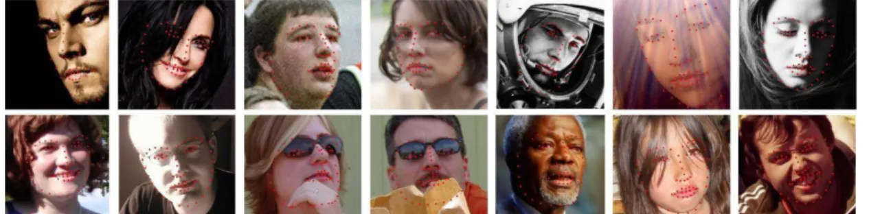
Figure 3.5: Output of coarse-to-fine convolutional network cascade model – (Database: 300-W (300 faces in wild) Key point detected: 68 Image / video: Images Only)
Explicit Shape Regression
Xudong Cao [35] presented very efficient and highly accurate Explicit Shape Regression approach. This model directly learns a vectoral regression function to infer the whole facial shape and explicitly minimize localization error in training data. The inherent shape encoded into the regressor in learning framework applied from coarse to fine to during testing. This approach uses two level boosted regression, a correlation-based feature and shape-indexed features selection method hence regression is more effective. It shows highly accurate and efficient results. Regression process is extremely fast in test 15 MS for 87 landmarks shape.
Figure 3.6: Output of explicit shape regression model – (Database: BioID, LFPW and LFW87 Key point detected: 5,29 or 87 Image / video: Images Only)
Constrained local models (CLM)
This model [36] is developed on Active Appearance Model (AAM). CLM differs from AAM because it is not a generative model for the whole face, instead it produces landmark templates iteratively and use a shape constrained search technique. The position vectors of the landmark’s templates are estimated using Bayesian formulation. The posterior distribution in Bayesian formula incorporates both the image information via template matching scores and the statistical shape information. Therefore, positions of new landmarks are predicted in the joint shape model and the light of the image, and then templates are updated by sampling from the training images.
Figure 3.7: Output of constrain local model – (Database: BioID and XM2VTS, Key point detected: 22 Image / video: Images Only)
Parameterized Kernel Principal Component Analysis (PKPCA)
Torre, et al [37] presented the parameterized kernel principle component analysis (PKPCA) model by extending KPCA to incorporate geometric transformation into formulation and applying gradient descent algorithm for fast alignment. This model differs from PCA because it can model non-linear structure in data in variant to rigid or non-rigid deformations. It does not require manually labeled training data.
Figure 3.8: Output of PKPCA model – (Database: CMU Multi-PIE, Key point detected: 46, Image / video: Images Only)
Multiple Kernel Learning
Rapp, et al, in [38] presented multiple kernel, it uses two patches on the face. One covers the eye region and the other covering the mouth region. In testing, pixels of a respective regions should be part of a target landmark, using the multi-resolution windows (progressively smaller nested windows) texture data is extracted that captures information from global to local view range. Every resolution level, information is passed into a different kernel and the convex combination of these kernels, instead of concatenating pyramidal information. For each
resolution level there is dedicated kernel which forms a multi-kernel SVM. The multi-kernel SVM is trained using center-surround architecture and the surround windows forming the negative examples. After the discovery of landmark points, without having any spatial relationship among them initially. To reach the plausible shapes, point distribution models are invoked. The point distribution models are particularly focusing to the mouth and to the eye-eyebrow pairs. The shape alternatives are evaluated using Gaussian mixture models (GMMs), so that the point combinations that possess the highest sum of SVM scores and that fit best to the learned models are selected.
Figure 3.9: Output of multiple kernel learning – (Database: Cohn-Kanade and Pose, Illumination and Expression (PIE), Key point detected: 17, Image / video: Images only)
Semi - Supervised learning
Tong, et al [39] address to the often imperfect and tedious task of manual landmark labeling, and to overcome this suggest a scheme to partly automate land-marking. In their method, a small percentage (e.g., 3%) of faces needs to be hand labeled, while most the faces are automatically marked. This is done by propagating the few exemplars landmarking information to the whole set. On the minimization of the pair wise pixel differences resulting in two error terms, the learning is based. The penalty in one term makes the warping of each un-marked image toward all other un-marked images, irrespective of the content they become more alike. While penalty in the other term controls the warping of un-marked images toward marked images. The warping function itself can be a piecewise affine warp to model a nonrigid transformation or a global affine warp for the whole face.
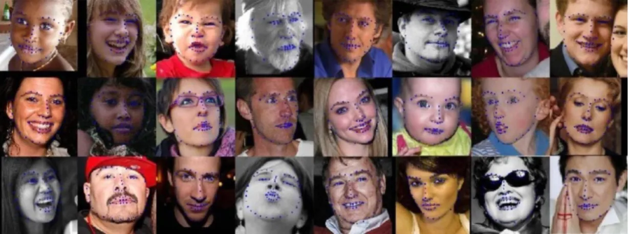
Figure 3.10: Output of semi supervised learning – (Database: Notre Dame, Caltech 101and FERE, Key point detected: 33, Image / video: Images only)
Bayesian Approach
Belhumeur in [40] presented a fully Bayesian approach to find landmark positions from local evidences. An interesting aspect about their work is that the local detector outputs are collected from a cohort of exemplars (sample faces with annotated landmarks), which provide non-parametrically the global model information. The local detector consists of a sliding window whose size is proportional to IOD and which collects SIFT features. In the next stage, the global detector models the configurational information of the ensemble of primary points. The joint probability of the location on ‘n’ landmarks and the vector of their local detectors outputs is maximized. This method surpasses in accuracy the performance of the manual landmarking in most of the 29 landmarks considered.
Figure 3.11: Output of Bayesian approach – (Database: BioID and LFPW, Key point detected: 29, Image / video: Images only)
Conditional Regression Forests
Dantone in [41] proposed pose-dependent landmark localization scheme that is achieved by conditional random forests. Conditional regression forests learn several conditional probabilities over the parameter space, and deals with facial variations in appearance and shape, while regression forests try to learn the probability over the parameter space from all face
images in the training set. The head pose is quantized into five segments of i) right profile ii) right iii) front iv) left and v) left profile faces and specific random forests are trained. Both texture and 2D displacement vectors that are defined from the centroid of each patch to the remaining ones described the local properties of a patch. Texture is described by normalized gray values in order to cope with illumination changes in addition to Gabor filter responses. Training of conditional random forests is very similar to random forests, except that the probability of assigning a patch to a class is conditioned on the given head pose. This method locates landmarks in a query image at real-time speed.
Figure 3.12: Output of conditional regression forests – (Database: LFW, Key point detected: 10, Image / video: Images Only)
Multi View
Zhanpeng Zhang, et al, in [42] presented a real time Multi-View facial landmark localization in RGB-D images. This system is able to estimate 3D head pose and 2D landmark localization. The model extracts random local binary patterns of different scales and estimate the facial parameters with hierarchical regression techniques. At first, 3D face positions and rotations are estimated via a random regression forest. Afterwards, 3D pose is refined by fusing the estimation from the RGB observation. The depth channel and RGB channel are used at different stages, the depth input is fed to the random forest for face detection and pose estimation at the beginning stage, the RGB input is fed to gradient boosted decision trees (GBDT) for head pose and hierarchical facial landmark location regression when the face is available. The pose estimation results from the depth and RGB inputs are weighted and combined to improve the precision.
Figure 3.13: Output of multi-view model – (Database: BIWI Kinect Head Pose, Key point detected: 13, Image / video: Images only)
Combinatorial Search and Shape Regression
Sukno in [43] have managed the combinatorial problem using RANSAC algorithm. First, they find out the reliable features using spin images as features and the missing are regressed using the multivariate Gaussian model encompassing all 3D landmark coordinates. The correct landmarks are sort out from the multitude of candidate points, all combinations of four points are used and RANSAC is used as the basis of the feature matching procedure. For the missing landmarks the median of the closest candidates is considered. The PCA instrumented shape fitting term for the detecting landmarks is has been used in the cost function consist of a part accounting for the reconstruction error, the other part accounts for the distance from the inferred landmarks to their closest candidates.
Figure 3.14: Output of combinatorial search and shape regression – (Database: FastSCAN, Key point detected: 8, Image / video: Images and video both)
Tree-structured models
estimation and facial landmarks localization. This algorithm is shape driven and local and global information are merged right from beginning. Since pose is part of estimation, the algorithm practically works as a multi-view algorithm. Multi-view implemented by considering several (30 to 60) local patches that are connected as a tree which collectively describe the landmark related region of the face.
Figure 3.15: Output of tree structured model – (Database: CMU MultiPIE and AFW, Key point detected: 61, Image / video: Images only)
Supervised Descent Method
Xuehan Xiong in [45] presented a Supervised Descent Method (SDM) for localizing facial landmarks. At first, it takes an image with manually labeled landmarks. Then it ran through training images to give initial configuration of landmarks. It uses SIFT function to extract initial landmarks. In training, SDM tries to minimize difference between manually labeled landmarks and initially located landmarks by SIFT (Δx). This method does not learn any shape or appearance model in advance from training data. The SDM learns a series of descent direction and re-scaling factors to produce a sequence of updates. SDM directly learns descent direction from training data by learning a linear regression between, (Δx) and difference of SIFT value of manually and extracted landmarks (ΔΦ). In testing, based on descent direction and re-scaling factors learn in training SDM estimates landmarks. SDM learns descent direction without computing Jacobian nor Hessian matrix, which are computationally expensive. SDM is fast and accurate.
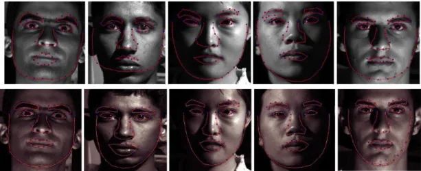
Figure 3.16: Output of Supervised Descent Method – (Database: LFPW and LFW-A&C, RU-FACS, Key point detected: 49, Image / video: Images and video both)
Methods and procedures
Introduction
As the idea was to test and gather data over a mensal period and that there is no such database available, we had to start first by gathering the necessary data. The data needed to be collected over a whole period, and each day, the women who participated in the experience had to come to the lab to take a picture in particular setting.
Once the data was collected, we needed first to prove that there is a perceptible change in the visual aspects of the face. A simple analysis of the results could give a hint that a change occurs during the period and therefore, fluctuant asymmetry studies could not take place over a simple photo of one day. Then we needed to landmark all faces manually to create a ground truth data base for comparison with automatic methods. This process was very time consuming because all and every single picture had to be marked manually and then reviewed for a second time for correction. Finally, different automatic landmark extraction methods had to be implemented and tested over our own database.
Data collection
50 women were photographed for 32 days, about 10 photos each day. From this set of pictures, we have chosen one best photo for each day and for each woman. Then they are normalized as much as possible for light and contrast.
All women were chosen from Portuguese nationality. They were all aged between 20 and 35 and they were all university students. All data about their sexual orientation, partners and contraceptive methods was collected for further analysis. The data base is not yet publicly available as the study is ongoing and legal permissions are not yet obtained.
Human rating
Once the data was collected, we needed first to prove that there is a perceptible change in the visual aspects of the face. Therefore, human raters had to rate the pictures of the same
woman over her mensal period. To do this, we developed a simple application that provides a list of photos of each girl ordered in a form page. The rating app is developed using C# and Mysql. This is a window form application programmed by C# and one form per girl. Each form includes 15 check boxes, which is connected to the database in Mysql, a timer and conditional next bottom and skip bottom. The app runs as an EXE file and outputs results in an excel file.
The main goal is to allow the ratters to choose in a short time best pictures of each woman during the mensal cycle. This will allow us to assess the existence of possible visual points which could appear during the hormonal modification in the body. As the data base is not yet publicly available and legal permissions are not yet obtained, we developed a desktop windows application witch only works with local IP.
At the first page of the application we classified raters by 4 factors. Raters can introduce themselves by gender, age, education and marital status. Having 2 categories of males and females’ raters allows us to make our database ready for comparing our results to other sexual attractiveness researches. Although most of our raters are university students or professors, regarding the fact that most of studies on attractiveness are based on age-controlled groups, we put 11 groups of ages between 15 and 75. In future work we will be able to find how much maturity affects the human opinion about attractiveness. Also, the last option is considered to determine if rater choices are influenced by marital status. The extraction of different classes of the ratters and the results they have obtained can also be a valuable data for future psychological work over who is really the receiver of the possible signs.
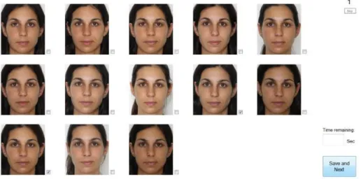
Each page includes 12 to 15 photos of one girl and each girl has 2 pages. All selected photos of each girl are placed in 2 pages randomly and each photo appears only one time. Therefore, the rater has a chance to see all photos of each girl taken over one month.
All photos are normalized as much as possible for light and contrast. But there is no preprocessing applied to change the skin color. All photos are face cropped to be in the same size and same head pose, to make the rater concentrate only on face attractions. Also, the app pages are very simple, neutral color and mostly filled by face photos, to avoid distractions.
more and not less, and it is not possible for the rater to go to the next page without choosing but he can skip the app and save his rating. All photos on each page are connected to the original one in the data base containing the photo dates. Therefore, when the checkbox of a photo is marked by the rater in the platform, the photo and photo date get one ’plus’ in database. At the end we have a list of data for each girl which contains photo name and photo dates. This list is ordered by number of times the photo was chosen.
Another feature of the app is a limited time for choosing. The rater has only 30 seconds on each page, to decide which photos are the most attractive ones. The idea behind the limited time is the fact that human brain makes up its mind up to ten seconds before actually realizing it [16].
Before starting the app, all raters are told that the goal is choosing the best photo of each girl in terms of attractiveness without considering any specific parameter, which means their first opinion is the best. That’s why at first glance, the rater’s brain would know what he is looking for. Therefor In the first few milliseconds of seeing each page, the rater realizes the best photo. But as long as the difference between photos in each page is very low, we gave 30 seconds to rostromedially prefrontal cortex of rater’s brain go a bit deeper and evaluate the decision with all judgment parameters available in the brain [17].
Figure 4.2: rating application, the example of girl’s photos page
Implementations
After some verification of existing methods and the available results, we decided to implement and test 3 methods. The methods were chosen by the following criteria:
• Available and verifiable literature and previous results • General towards specialized
• Estimated Precision
We, therefore, chose to test 3 methods:
• Active appearance Model -AAM
• Convolutional Neural Networks -CNN • Regression Trees from Dlib library –Dlib
Active appearance models
Facial landmark point extraction is a key step in facial image representation and analysis. The Active Appearance Model (AAM) proposed by Cootes et al [46] is a powerful object description method that is commonly used for facial landmark points extraction AAM fitting is
a non-linear optimization problem. Different optimization approaches have been proposed to find the best model parameters that result in minimum error between the synthesized appearance models obtained from the AAM and the input image. In general, due to variation of camera view angle, resolution and focal distance, facial images have different scaling, rotation, and translations. In order to remove global shape variations, all shapes are normalized, and the modeling is only concerned with local shape deformation. Therefore, it is necessary to combine a global shape transformation with the normalized AAM. The global shape transformation is often a 2D similarity transformation. Finding optimal parameters of the global transformation improves the accuracy of fitting in representing novel facial images with different shape and pose variations. Traditionally, the stochastic gradient descent algorithm or iteratively incremental additive techniques are used to update the AAM parameters to fit onto novel images. The fitting problem can also be viewed as finding a model instance similar to the given facial image and therefore it can be considered as an image alignment problem.
Figure 4.3: AMM fit on a given face
AAM consists of a shape component and an appearance component obtained from a set of annotated landmark points in training images. Let’s assume we are given a training facial image set with annotated shapes defined as: S = (X1, Y1, X2, Y2, ..., Xv, Yv)T . The training images are first normalized and aligned using iterative Procrustes analysis. This step removes variations due to a chosen global shape normalization transformation so that the resulting model can efficiently consider local and non-rigid shape deformation. We then can combine the resulting AAM with a global transformation. Afterwards, Principal Component Analysis
(1)
where the base shape S0 is the mean shape and the vectors Si are n eigenvectors
corresponding to the n largest eigenvalues. Then, all the training images are normalized by warping them into the base shape S0, using piecewise affine warp, and the appearance model is
defined as:
(2)
where A0 is the mean appearance and the vectors Ai are the m eigenvectors corresponding
to the m largest eigenvalues. The goal of fitting is to find a model instance that can efficiently describe the object (e.g. face) in a given image. Thus, it can be considered as an image alignment problem. In other words, we want to find the model instance M(W(x; p)) = A(x) as similar as the image I(x). In general, facial images have different scaling, rotation, and translations. Therefore, it is necessary to combine a global shape transformation with the normalized AAM. If we consider the global shape transformation as N(x; q), we want to minimize the error between the template and I (N(W(x; p) ; q)). Considering global shape transformation, the objective of the fitting process is to find p and q in order to minimize the error image as:
(3) 𝐸(𝑥) = ∑ [𝐴0(𝑋) − 𝐼(𝑁(𝑊(𝑥; 𝑝); 𝑞))]2
𝑥∈𝑠0
Which is a non-linear least square problem. We can have different definitions for the global transformation N(x; q). In [47], a set of 2D similarity transformations as a subset of piecewise affine warps is defined. This representation of N(x; q) is similar to W(x; p) and therefore similar analysis on the shape parameters p can be applied to q. If we assume that the
two sets of shape vectors Si and Si* are orthogonal to each other, we can add the four 2D similarity vectors Si* to the beginning of AAM shape vectors Si [47] and model any given shape as: In practice, Si and Si*are not quite orthogonal to each other.
This can either be ignored when the size of Si is small or the complete set of Si and Si*can be orthonormal zed preferably.
In [48], Baker et al. relate AAM to the Lucas-Kanade algorithm. They proposed the Inverse Compositional Algorithm (ICA), in which they find shape variation on the template and compose the inverse of that with the current shape. Therefore, many computationally expensive tasks are recomputed. In [47], appearance variation is considered in the fitting by finding shape parameters in a linear subspace where the appearance variation is ignored and then “projected out” to the full space with respect to the appearance eigenvectors. The method is more generic compared with the ICA, but the fitting is not accurate when applied to subjects that are not similar to subjects in the training set. The “projecting out” approach is called PO in the rest of this paper. In [49] Simultaneously Inverse Compositional (SIC) method is introduced, which is more generic. In this method the fitting procedure minimizes the error between[𝐴0(𝑥) + ∑𝑚𝑖=1(𝜆𝑖+ Δ𝜆𝑖)𝐴𝑖 and I(N(W(x;p) ; q)), where Ai are m appearance eigenvectors correspond
to the m largest appearance eigenvalues, and (λi +Δλi) are parameters of appearance that are found simultaneously with respect to the Δp. As the appearance parameters are optimized in each iteration, both steepest descent and the Hessian matrix (H) should be calculated in each iteration, and therefore the method is slower. In [49] the PO is compared with the SIC, and the SIC is reported more accurate in modeling unseen subjects.
Convolutional neural networks and deep learning
Architecture Overview
Recall: Regular Neural Nets: Neural Networks receive an input (a single vector) and transform it through a series of hidden layers. Each hidden layer is made up of a set of neurons, where each neuron is fully connected to all neurons in the previous layer, and where neurons in a single layer function completely independently and do not share any connections. The last fully connected layer is called the “output layer” and in classification settings it represents the class scores.
Regular Neural Nets don’t scale well to full images. In CIFAR-10 dataset, images are only of size 32x32x3 (32 wide, 32 high, 3 color channels), so a single fully connected neuron in a
first hidden layer of a regular Neural Network would have 32*32*3 = 3072 weights. This amount still seems manageable, but clearly this fully connected structure does not scale to larger images. For example, an image of more respectable size, e.g. 200x200x3, would lead to neurons that have 200*200*3 = 120,000 weights. Moreover, we would almost certainly want to have several such neurons, so the parameters would add up quickly! Clearly, this full connectivity is wasteful, and the huge number of parameters would quickly lead to overfitting.
3D volumes of neurons: Convolutional Neural Networks take advantage of the fact that the input consists of images and they constrain the architecture in a more sensible way. In particular, unlike a regular Neural Network, the layers of a ConvNet have neurons arranged in 3 dimensions: width, height, depth. (Note that the word depth here refers to the third dimension of an activation volume, not to the depth of a full Neural Network, which can refer to the total number of layers in a network.) For example, the input images in CIFAR-10 are an input volume of activations, and the volume has dimensions 32x32x3 (width, height, depth respectively). As we will soon see, the neurons in a layer will only be connected to a small region of the layer before it, instead of all of the neurons in a fully connected manner. Moreover, the final output layer would for CIFAR-10 have dimensions 1x1x10, because by the end of the ConvNet architecture we will reduce the full image into a single vector of class scores, arranged along the depth dimension. Here is a visualization:
Figure 4.5: A ConvNet arranges its neurons in three dimensions (width, height, depth), as visualized in one of the layers. Every layer of a ConvNet transforms the 3D input volume to a 3D output volume of neuron activations. In this example, the red input layer holds the image, so its width and height would be the dimensions of the image, and the depth would be 3 (Red, Green, Blue channels)
Parameter Sharing. Parameter sharing scheme is used in Convolutional Layers to control the number of parameters. Using the real-world example above, we see that there are 55*55*96 = 290,400 neurons in the first Conv Layer, and each has 11*11*3 = 363 weights and 1 bias. Together, this adds up to 290400 * 364 = 105,705,600 parameters on the first layer of the ConvNet alone. Clearly, this number is very high.
It turns out that we can dramatically reduce the number of parameters by making one reasonable assumption: That if one feature is useful to compute at some spatial position (x,y), then it should also be useful to compute at a different position (x2,y2). In other words, denoting a single 2-dimensional slice of depth as a depth slice (e.g. a volume of size [55x55x96] has 96 depth slices, each of size [55x55]), we are going to constrain the neurons in each depth slice to use the same weights and bias. With this parameter sharing scheme, the first Conv Layer in our example would now have only 96 unique set of weights (one for each depth slice), for a total of 96*11*11*3 = 34,848 unique weights, or 34,944 parameters (+96 biases). Alternatively, all 55*55 neurons in each depth slice will now be using the same parameters. In practice during backpropagation, every neuron in the volume will compute the gradient for its weights, but these gradients will be added up across each depth slice and only update a single set of weights per slice.
Notice that if all neurons in a single depth slice are using the same weight vector, then the forward pass of the CONV layer can in each depth slice be computed as a convolution of the neuron’s weights with the input volume (Hence the name: Convolutional Layer). This is why it is common to refer to the sets of weights as a filter (or a kernel), that is convolved with the input.

![Figure 4.6: Example filters learned by Krizhevsky et al. Each of the 96 filters shown here is of size [11x11x3], and each one is shared by the 55*55 neurons in one depth slice](https://thumb-eu.123doks.com/thumbv2/123dok_br/18118386.869494/41.893.153.747.131.362/figure-example-filters-learned-krizhevsky-filters-shared-neurons.webp)

