Low reynolds propellers for increased quadcopters endurance

(1)

Engenharia

Low Reynolds Propellers for Increased

Quadcopters Endurance

Hélices de Baixo Reynolds para Aumento da Autonomia

em Quadricópteros

Isa Diana de Sousa Baptista Morais Carvalho

Dissertação para obtenção do Grau de Mestre em

Engenharia Aeronáutica

(2º ciclo de estudos)

Orientador: Prof. Doutor Miguel Ângelo Rodrigues Silvestre

(2)

(3)

III

“Para ser grande, sê inteiro: nada Teu exagera ou exclui. Sê todo em cada coisa. Põe quanto és No mínimo que fazes. Assim em cada lago a lua toda “Brilha, porque alta vive.” Ricardo Reis, Odes

(4)

(5)

V

Acknowledgements

At this stage there are many people to whom I would like to thank for their dedication on this great journey.

First of all I would like to thank Professor Miguel Ângelo Rodrigues Silvestre for his support, work, dedication and knowledge, otherwise this project would have been compromised. To my course colleague, PhD student, João Morgado for his grandiose availability to transfer me his knowledge, for supporting every time there were doubt and for providing the software developed by himself for the realization of my work.

To my parents for all their love, sweetness, dedication and financial support given to me during all these years and whom in their absence I would not be able to overcome this particular chapter of my life.

To my sisters, for all their love and for always believe me during my academic route. To my boyfriend for all his love, patience and unconditional support.

To the rest of my family members and friends that always supported me and believed me during this period.

(6)

(7)

VII

Resumo Alargado

O estudo e o desenvolvimento de pequenas aeronaves não tripuladas (UAV’s) tem crescido grandemente nestes últimos 20 anos. Em relação às aeronaves de asas rotativas este desenvolvimento é devido à sua enorme manobrabilidade, à sua capacidade de pairar no mesmo lugar e o facto de terem a habilidade de descolar e aterrar na vertical. A nível académico, o estudo dos quadricópteros, tem aumentado significativamente, principalmente pelo facto de serem aeronaves de extrema simplicidade mecânica, de apresentarem grande mobilidade e estabilidade, de acarretarem custos de manutenção/aquisição relativamente baixos comparativamente com outras aeronaves, pela sua facilidade de utilização em ambientes fechados e ainda, por apresentarem certa segurança na presença de seres humanos.

Os quadricópteros, são aeronaves que têm inúmeras aplicações: investigação, operações militares, busca e de salvamento, e ainda em aplicações comerciais (passatempo para pessoas aficionadas nestas aeronaves). [17]

Com a presente dissertação de mestrado em Engenharia Aeronáutica pretende-se contribuir para o desenvolvimento e investigação em quadricópteros de grande autonomia. Nesta dissertação é feita, inicialmente, uma abordagem ao tema em estudo, onde são mencionados os principais componentes (hélice, motor e bateria) para quadicópteros de grande autonomia e os avanços conseguidos pelo sector aeronáutico nesta vertente e as possíveis aplicações dos mesmos. Posteriormente, é feita uma descrição do programa utilizado para a execução do trabalho de análise de hélices existentes e projecto de uma nova hélice para uma maior autonomia, desde a descrição do código à formulação teórica. É realizada a validação do mesmo programa, com recurso a uma hélice já existente, a hélice ACP Slow Flyer 10x7, cujos dados constam do UIUC propeller database [13]. De seguida, é elaborada a análise para uma hélice de passo mais curto, a APC Slow Flyer 11x4.7, sendo esta utilizada como referência para a criação de uma nova hélice. O processo de projecto aerodinâmico da nova hélice é descrito minuciosamente, desde a parte conceptual, a selecção do perfil alar, o dimensionamento com o programa QMIL, a respectiva análise realizada no programa JBLADE e as respectivas comparações entre as hélices em questão: a hélice de referência e a nova hélice criada.

Palavras-chave

Quadricópteros de grande autonomia, hélice, asa rotativa, autonomia, perfis de baixo Reynolds.

(8)

(9)

IX

Abstract

With this MSit c. Dissertation in Aeronautical Engineering is intended to contribute to the research and development of long endurance quadcopters. In this dissertation, initially, the topic study is introduced and the principals components (propeller, motor and battery) for greater autonomy quadcopters are described along with the advances made by the aeronautical sector in this strand and the possible applications. Posteriorly, a description of the program used for the analysis of existing propellers and new designs is given, and its validation is performed with the experimental data set of an existing propeller, the propeller APC Slow Flyer 10x7 made available by UIUC propeller database. Then, analysis of a lower pitch propeller, the APC Slow Flyer 11x4.7 is presented and used, as the point of reference for the creation of an improved long endurance quadcopter propeller. The process of creation of a new propeller is thoroughly described, from the conceptual approach, the airfoil selection, the design for minimum induced loss with QMIL, to the respective analysis realized on the program JBLADE and the respective comparison between the propellers in question: the base propeller and the created propeller.

Keywords

(10)

(11)

XI

List of Figures

Figure 1.1 – Bothezat Helicopter.

Figure 1.2 – Autonomous quadcopter that use a smartphone to navigate. Figure 2.1 - Quadcopter + configuration.

Figure 2.2 – Quadcopter X configuration. Figure 2.3 – Quadcopter principal components. Figure 2.4 – Example of a fuel cell battery.

Figure 2.5 - First solar powered quadcopter in the world. Figure 2.6 – Electric rotorcraft with 18 motors, VC200.

Figure 3.1 - Decompositions of total blade-relative velocity W at radial location r. Figure 3.2 - Blade geometry and velocity triangle at an arbitrary radius blade position. Figure 3.3 - Example of a blade displayed in JBLADE.

Figure 3.4 - JBLADE code structure.

Figure 3.5 – Airfoil extracted from GETDATA (dots) versus Smoothed airfoil obtained in JBLADE (continuous line).

Figure 3.6 - Smoothed airfoil obtained in JBLADE.

Figure 3.7 – Propeller incidence and chord distribution for the APC SF 10x7 propeller as presented in UIUC Propeller Database.

Figure 3.8 – APC SF 10x7 calculated versus measured thrust coefficient in function of advance ratio at 3000 RPM.

Figure 3.9 – APC SF 10x7 calculated versus measured power coefficient in function of the advance ratio at 3000 RPM.

Figure 3.10 - APC SF 10x7 calculated versus measured propeller efficiency in function of the advance ratio at 3000 RPM.

Figure 3.11 - APC SF 10x7 calculated versus measured validation of calculations: Thrust coefficient versus advance ratio to range of 6000 RPM.

Figure 3.12 - APC SF 10x7 calculated versus measured validation of calculations: Power coefficient versus of the advance ratio to range of 6000 RPM.

Figure 3.13 - APC SF 10x7 calculated versus measured validation of calculations: propeller efficiency versus advance ratio to range of 6000 RPM’s.

Figure 3.14 – Thrust coefficient versus advance ratio to APC SF 10x7. Figure 3.15 – Power coefficient versus advance ratio to APC SF 10x7. Figure 3.16 – Propeller efficiency versus advance ratio to APC SF 10x7. Figure 3.17 – APC Slow Flyer 10x7.

(14)

XIV

Figure 3.18 – ACP Thin Electric 10x7. The graphic represents the thrust coefficient versus advance ratio at different rotational speeds.

Figure 3.19– APC Thin Electric 10x7.

Figure 3.20– ACP Sport 10x8. The graphic represents the thrust coefficient versus advance ratio at different rotational speeds.

Figure 3.21 – APC Sport 10x8.

Figure 3.22 - Propeller incidence and chord distribution for the APC SF 11x4.7 propeller as presented in UIUC Propeller Database.

Figure 3.23 – Thrust coefficient versus advance ratio to APC SF 11x4.7. Figure 3.24 – Power coefficient versus advance ratio to APC SF 11x4.7. Figure 3.25 – Propeller efficiency versus advance ratio to APC SF 11x4.7.

Figure 4.1 – Drag polar of benchmark propeller airfoil for the 0.75R blade position and operating Reynolds Number of 123864.

Figure 4.2- CL distribution along the blade position for the benchmark propeller in the static thrust condition at 6000 rpm.

Figure 4.3 – The three analysed profiles (benchmark propeller airfoil, SD7003-085-88 and the MH42 8.94%).

Figure 4.4 – Comparison of CL/CD between the three airfoils to Reynolds Number of 100000. Figure 4.5 – Curves that allow to represent airfoil characteristics in QMIL.

Figure 4.6 – Drag polar function used for the MH42 8.94% airfoil in QMIL for Reynolds number of 100000.

Figure 4.7 – Lift curve used for the MH42 8.94% airfoil in QMIL for Reynolds number of 100000. Figure 4.8 – First sketch of the AE propeller.

Figure 4.9 - CL distribution along the blade position for the AE propeller in the static condition.

(15)

(16)

XVI

List of Tables

Table 1.1 - Typical propellers pitch and diameter used in common quadcopters. Mean p/D=0.456

Table 3.1 - Values of the viscosity and density of air at standard atmosphere. Table 3.2 – APC 10x7 parameters for 3000 RPM and 6000 RPM.

Table 3.3 - APC 11x4.7 parameters for 3000 RPM and 6000 RPM. Table 4.1 – The data benchmark propeller.

(17)

(18)

XVIII

List of Notations

aa – Axial Induction Factor

at – Tangential Induction Factor A – Propeller Disk Area = B – Number of Blades

c – Blade Local Chord [m] Ca – Axial Force Coefficient CD – Airfoil Drag Coefficient CD0 – Minimum Drag Coefficient

CD2l – Drag Coefficient quadratic parameter CD2u – Drag Coefficient quadratic parameter CL – Airfoil Lift Coefficient

CL0 – Lift Coefficient at zero pitch CLCD0 – Lift Coefficient at Minimum Drag CLDES – Lift Coefficient to maximum efficiency CLmax – Maximum Lift Coefficient

CLmin - Minimum Lift Coefficient CLα – Lift Curve

Ct – Tangential Force Coefficient – Power Coefficient

– Thrust Coefficient D – Propeller diameter [m] F – Prandtl’s Factor K – Velocity Gradient

Kv - Motor Velocity Constant [rpm/V] Ma – Mach Number

N – Propeller Rotation Speed [Rev/s] p – Propeller Pitch

P – Required Propeller Shaft Power [W] Q – Required Propeller Shaft Torque [Nm] r – Radius of blade element position [m] R – Propeller Radius [m]

Re – Reynolds Number

ReRef – Reynolds Number Reference RPM – Revolutions per Minute T – Propeller Thrust [N]

(19)

XIX

V – Propeller airspeed [m/s] Va – Induced Axial Velocity [m/s] Vt – Induced Tangential Velocity [m/s] W – Element Relative Velocity [m/s] Wa – Axial Velocity Component [m/s] – Average axial velocity [m/s]

Wt – Tangential velocity component [m/s] α – Angle of Attack

Β – Pitch or Blade Angle Φ – Inflow Angle

θ – Incidence Angle (degrees) μ – Air Viscosity [Pa.s] ρ – Air density [Kg/m3_] Ω – Angular Velocity [1/s] Ωr – Local rotation Speed [m/s] – Local rotor solidity ratio

Acronyms List

APC – Advanced Precision Composites BEM – Blade Element Momentum Theory ESC – Electronic Speed Controller FPV – First-Person View

IMU – Inertial Measurement Unit MAV- Micro Air Vehicle

MTOW – Maximum Take-Off Weight RC – Radio Control

UAV – Unmanned Aerial Vehicle UBI – University of Beira Interior

UIUC - University of Illinois at Urbana-Champaign

(20)

(21)

1

1. Introduction

The first successful helicopter was the Bothezat built in 1920’s by George de Bothezat for United States Army Air. It was an experimental quadrotor helicopter with four six-bladed rotors, built with truss beams connected by piano wire. The Bothezat machine made its first flight on 1922 and hovered to a height of 1.8 meters. In the following year, were held hundreds of flight tests, where several records were taken: load (4 passengers + pilot), duration (2 minutes and 45 seconds) and altitude (9.1 meters). [18]

Figure 1.1 – Bothezat Helicopter. [18]

Since the mid-1990s, the study and the development of small UAVs has been rising due to military interest and funding [1-31]. This research and evolution in the case of rotorcrafts were due to their enormous maneuverability and their abilities to hover in place and to land and take-off vertically. The quadrotor is an emerging MAV that may be used in many situations. Their usefulness as aerial imaging tools has been proven over these years. However, new researches are allowing quadrotors to explore unfamiliar environments, to maneuver in environments with adverse conditions and to communicate with other autonomous vehicles intelligently. It is believed that combining all of these abilities, these MAV’s will be able to perform autonomous missions, currently unthinkable to any other vehicle.

Like conventional helicopters, quadcopters can hover but have other advantages like improved stability and their designs are mechanically simple (having no swash-plate mechanism) which means that this configuration allows the use of smaller propellers and consequently results in a minor amount of kinetic energy stored in the blades which reduces possible damages if the blades collide with something during the flight. These characteristics also simplify the design and maintenance of the vehicle [2]. A major limitation of a quadcopter is its endurance. Generally, a quadcopter flight time is around 20 minutes but if

(22)

2

they are carrying a significant payload fraction, the flight time is substantially reduced [3]. Record flight times when carrying only batteries are close to one hour.

It is important to research and development in this type of aircraft in order to optimize and develop components/concepts to ensure a better performance and endurance without increasing the production costs. An increased endurance would allow extending significantly the potential of quadcopters for useful UAVs applications.

According to the deputy chief fire officer of the West Midlands fire brigade:

“This is fantastic new technology that will provide real benefits when we are tackling a range of emergency situations. Being able to look down on the scene will allow us to get a full picture of the incident and the surrounding environment, which will aid incident commanders to make vital, potentially life-saving decisions.” – PA News

Literature review makes believe that this type of aircraft has the biggest advantage for autonomous applications and could be useful for important roles such as disaster response, first responders, to survey the inside of buildings, to patrolling forests which can help improve any living life quality. [9]

Figure 1.2 – Autonomous quadcopter that use a smartphone to navigate. [9]

1.1 Problem Motivation

Even though aircraft propellers have been designed for over a century, investigations and developments on the performance and the design of propellers are extremely important. The

(23)

3

interest in propeller propulsion is due to its huge efficiency to lower flight speeds comparatively with turbofan propulsion. [20]

Quadcopters are typically fixed-pitch aircrafts and they are becoming more and more popular due to their mechanical simplicity relative to other hovering aircraft. They were made possible with the evolution in electric motors, in particular the brushless outrunners, that offered reliability, efficiency, high power to weight ratio and direct drive. This simplicity places limits on the types of maneuvers possible to fly. One such limitation is the unability to perform autorotation.

One of the biggest problems of the quadcopter is its short endurance. As any aircraft, endurance is a point of utmost importance thus it is necessary to have a thorough study of each of the components that affects this performance parameter.

This thesis explores the extent to which a new propeller with different characteristics from those already in use could improve the common quadcopter's endurance.

1.2 Dissertation Structure

This dissertation is organized in five chapters. In chapter 1, an introduction to the topic, motivation and the description of the dissertation structure is presented. Chapter 2 is where the theory subjacent to the research problem is presented, in which the principals components to the long endurance quadcopters are described. In this chapter the state-of-art related to this topic (new discovers and possible application on aeronautic sector) is also included.

In chapter 3 the code used for the analysis of the existing and designed propellers is described, the JBLADE. The validation of JBLADE through the UIUC propeller database experimental data for the APC Slow 10x7 propeller is performed. It is also in this chapter that the analysis of the propeller APC Slow Flyer 11x4.7 using the software JBLADE is done. This served as reference for the creation of the new propeller.

In chapter 4 are contained all the steps of creation of the new propeller since the airfoil selection, design for minimum induced loss with QMIL, to its analyses on the software JBLADE and the comparison with the reference propeller.

(24)

4

2. A Long Endurance Quadcopter

2.1. The Multicopter Concept

Multicopter or multirotor is generally a small RC rotorcraft with four or more rotors. Through the variation of the rotational speed of each rotor (to change the thrust and torque produced by each one) the control of aircraft motion is obtained, i.e., roll, pitch, yaw.

Multicopters are special aircrafts and they do not depend on mechanical swashplates, tail rotors, or coaxial rotors to achieve a controlled flight. There is no specific definition for multicopter. According to Paul Gentile, “A heavier-than-air aircraft that has two or more

usually symmetrically placed rotors and whose control of pitch, roll, yaw, and lift are achieved solely through the variation of the speed (rpm) of each rotor and whose flight stabilization is through a combination of electro/mechanical sensors and computing devices.” [4]

Mulicopter are tipically of the type: quadcopter (four rotors), hexacopter (six rotors) and octocopter (eight rotors). Due to the axisimmetry and to the distance from the rotors to centre of gravity, any pitch or roll motion are well damped because such motions will dictate the change in the mean angle of attack of opposing rotors blades. This gives the multicopters exceptional stability. On the other way around, by the same reason, control moments are easily obtained by changing the thrust of opposing rotors.

RC multirotors are increasingly used for making aerial videos and aerial photography. The First-Person View (FPV) is a type of remote-control flying that has been gaining popularity. It involves mounting a small video camera and analog television transmitter on a remote control (RC) aircraft and viewed on a screen or with goggles. Flying in FPV, offers virtual reality experience of actually flying in the aircraft and no need to look at the aircraft. [19]

Due to ease of control and construction multicopters are widely used as a way of entertainment to fly outdoors or indoors [16] and have become popular in RC aircraft projects [19].

One important advantage of multicopters is that by dividing the same thrust by multiple rotors/propellers, the total weight of the rotors is greatly reduced compared to a conventional single rotor providing all the wight balancing thrust. This is due to the scaling effect of propellers thrust and structural weight.

(25)

5 2.2. State of the Art

The quadcopter is a multicopter with four rotors and its movement is controlled by variation of relative thrusts of each rotor through the change in each rotor’s rotational speed. The rotors are aligned in a square and two of them spin clockwise and the other two spin counter clockwise.

There are two quadcopters configurations, the + and the x.

Figure 2.1 - Quadcopter + configuration [5].

(26)

6

As one can see in figures 2.1 and 2.2, in both configurations two rotors rotate in clockwise direction, while the other two motors spin in counter clock wise but the main difference between these two configurations is how the engines are controlled. The + configuration can be controlled in pitch and yaw with only one motor providing extra thrust. In the X configuration, these functions are always ensured with two motors. Although the quadcopters are prone to be very stable, in the pitch and roll and yaw rates around the hovering flight condition, they neutrally stable and very responsive to slight changes in the motors throttle setting. It would be nearly impossible to manually control the 4 rotors to keep the thrust balanced among the four rotors and thus maintaining a manually controlled flight. So, common quadcopters have a stability augmentation system (autopilot) based in an IMU and a controller.

The components affecting the endurance of the quadcopter are:

Rotors/Propellers:

The choice of a quadcopter propeller is extremely important because this component determines the power consumption for the required thrust. The average thrust required for each rotor is roughly one fourth of the quadcopter’s MTOW. Typically, two bladed propellers are used; they tend to be more efficient since the blades’ operating Reynolds number for a given motor speed is increased compared with 3 or more blades propellers with the same motor solidity, . Single blade propellers would allow increasing the blade Reynolds number even further but would require a counter-weight. The diameter influences the performance and the quadcopter’s dynamic behaviour, the larger diameter the higher the static thrust efficiency (T/P) for a given thrust but the maximum pitch and roll rates will be slower. According to Gary Mccgray (a forum blogger), “My ARF F450 Flamewheel QuadCopter came

with 10" light weight and not very efficient props. I replaced the propellers with much stronger and better designed 11" Carbon GemFans and achieved an extra 2+ minutes per flight and the copter is quieter and more stable.” One must take into account that this 2

minutes increase in the flight time means more than 10% in endurance because the average quadcopter flight time is quite low.

In accordance with Oscar Liang [10], the standard propellers for a quadcopter could be EPP0938 and EPP0845 to use in smaller quadcopters; APC SF 1047 and EPP1045 (the most popular one) are applicable in mid-sized quadcopters; EPP1245 is used in larger quad copters that demands big amounts of thrust. However, RCPowers recommends APC SF propellers because they provide good power in a broad RPM range [23]. According to this, as summarized in Table 1.1, the mean p/D used in common quadcopter designs is 0.456. The recommended EPP propellers are similar in airfoils and blade design to APC SF propellers but cheaper while

(27)

7

APCs are built with better materials such that they seem much more rigid than EPP propellers.

p

D

p/D

4.5

8 1.777778

3.8

9 2.368421

4.7

10 2.12766

4.5

10 2.222222

4.5

12 2.666667

Table 1.1 - Typical propellers pitch and diameter used in common quadcopters. Mean p/D=0.456

The quadcopter propellers are almost always fixed pitch [31]: as mentioned, two of them will spin clockwise and the other two will spin counter clockwise. Due to this arrangement concept, this allows all control motions of a traditional helicopter: hover, forward and backward motion, left and right as well as yaw control.

One important aspect to consider is that of the balancing of the propeller. An unbalanced propeller produces excessive vibration and causing premature failures on parts and motor bearings and distorts the readings taken by the IMU sensors (inaccuracy). A balanced propeller is fundamental to the quadcopters stability, because the vibration produced is lower (more stable aircraft) and the current consumption is reduced (increased endurance). [21]

Batteries:

The lithium based batteries are the preferred energy source for quadcopters because they provide elevated discharge rates and good ratio energy storage/weight (specific energy). Generally, the battery recommend is a lithium polymer battery (LiPo) due to its high specific energy and current ratings. The nickel metal hydride batteries (NiMH) are another option of choice because they are cheaper, less limited in number of charge discharge cycles useful life, have the highest specific energy after the lithium based batteries but they are heavier than the lithium batteries and have lower tolerance to overcharging than the Nickel cadmium batteries. The NiCads could be used for small to medium size quadcopters but their small specific energy puts a severe limit to the quadcopters endurance. This type of battery has the highest current output and a more affordable price than the NiMH batteries. [6]

For long endurance quadcopters, the specific energy is the driving parameter, the higher the better. So, typically, the LiPo 3SP1 battery configuration (three cells connected in series and a single one in parallel) and the nominal motor voltage value is thus 11.1V.

(28)

8

A crucial endurance parameter related to the battery is the battery weight fraction. A high battery weight to MTOW allows a higher endurance.

Motors:

Generally, the choice of the motor is driven such that it matches with the chosen propeller. The most common motors used in quadcopters are rare earth permanent magnet three phased high pole number brushless outrunners motors. These became very popular with RC aircraft hobbyists because of their efficiency in direct drive applications, power to weight ratio, simplicity and longevity in comparison to traditional brushed motors. The fact that no power of loss occurs neither in the brushes nor in reduction gears like traditionally happened with the brushed DC motors, makes the brushless motors more energy efficient thus, increasing the quadcopters endurance. One of the most important specifications of the motors besides the peak efficiency is the KV constant rating that specifies how many

revolutions per minute (RPMs) they will turn per volt of input energy [10]. For a fixed input voltage, motor efficiency, power and weight, a smaller Kv will turn a larger diameter propeller. As explained in section 4.1, a larger propeller will require less power for the same thrust thus increasing the quadcopter’s endurance. This generally pushes the quadcopter builder to use propellers of excessive diameter for small weight motors which can perform with excessive current, overheat and be very inefficient. It can, in a longer endurance application burn up the motor. However, an oversized motor will be heavy thus requiring higher thrust and power. Nevertheless, it can be profitable to used oversized motors to drive larger propellers. Therefore, as previously mentioned, the motors must match the propeller in use. A smaller propeller demands a higher Kv motor because they should spin faster to produce equivalent lift. Smaller propellers have reducem moment of inertia thus providing faster thrust changes, e.g., for an acrobatic quadcopter).

Electronic Speed Controller (ESC):

The Electronic speed control is the motor’s controller board that has a battery input and a three phase output to feed the motor windings which controls the speed of the motor and its direction based on the throttle that the autopilot is setting [10]. These controllers perform the function of the brushes in the brushed motors to connect the right windings at the right moments. Typically, sensorless ESCs are used. In this case, the synchronization with the motor is achieved by the controller measuring the to electromotive force in the phase windings that is not being fed in each moment. One ESC is used to each of the four motors. The most important factor in selecting an ESC is its maximum current specification. This is the maximum electrical current that the ESC can handle to satisfy the necessity of providing electrical power to the motor. However, if the amperage rating is not high enough it can overheat [24-25]. It turns out that using low partial throttle to handle big propellers while limiting the motor current within motor’s maximum current specification can significantly

(29)

9

increase the instantaneous current handled by the ESC. The reason for this is that the electrical power supplied to the motor is controlled by a high frequency PWM. So, in low partial power, the winding are only connected to the battery for a fraction of time meaning that to achieve a given average current, the instantaneous current must be inversely proportional to the throttle fraction in use. The consequence of selecting the ESC for average maximum current instead of maximum instantaneous current is that the ESC overheats. Besides the possibility of overheat failure, the ESC efficiency is obviously lower when heat is being generated by the ESC. The endurance in such a condition is clearly compromised.

Figure 2.3 – Quadcopter principal components. [29]

Structure:

The basic structure consists of four arms connecting the rotors to the center of gravity. The structure’s weight is an important factor for the quadcopter’s endurance since larger weight mean larger required thrust and more power. As with other aeronautical applications, materials with higher specific strength provide the lower structural weight. Currently the carbon fiber/epoxy composites materials are the usual choice.

The aerodynamic design of the structure arms can influence the vertical drag generated by the induced velocity of the propellers. The vertical drag adds to the quadcopters weight for the required hovering thrust. Structure arms with low drag sections provide smaller drag. The use of increased propellers’ diameter for the same thrust reduces the structures arms drag, although it increased the required structure arm length and weight.

Others:

Other factors that affect the quadcopters’ endurance are mostly the weight of systems like the autopilot and the payload systems. With miniaturization, these have been becoming

(30)

10

smaller and lighter with time thus allowing to increase the quadcopters’ battery weight fraction.

2.3. Possible Breakthroughs for Longer Endurance Quadcopters

The prospects to improve the quadcopter endurance are base on the components described in the previous section. Regarding the energy storage device, studies make believe that the new batteries generation will perform twice or triple better than today’s Lithium batteries. [6] The fuel cell batteries are a possible future alternative to batteries regarding the specific energy of the energy storage device. They have been in constant improvement in recent years and in a few years it will be a type of energy storage device accessible for everyone. The drawback of fuel cells is that although the current models have large specific energy, they still lack on specific power for a quadcopter application.

One definite advantage of carrying fuel as an energy storage mean is that the aircraft’s weight is reducing with flight time thus increasing largely the vehicle’s endurance.

Combustion engines quadcopters are generally not considered a feasable solution if the engines were to drive each propeller independently because of the lack of engine reliability and sensitivity to operating conditions making an unreliable throttle response for even the autopiloted stability and control. Nevertheless, a central engine/generator hybrid solution with a possible buffer battery bank could be considered. One obstacle to such a solution is the increase in the quadcopter size and weight making the variable pitch rotor/propeller a requirement for quick enough thrust control. On the other hand, the current simplicity and reliability would be reduced with such a concept.

Figure 2.4 – Example of a fuel cell battery. [6]

One innovation worth mentioning is the first solar powered quadcopter in the world by students of Queen Mary University of London. This project can be an asset for environmental

(31)

11

aircraft friendly developing and space exploration [7]. Needless to say, that the endurance is greatly improved with such an external energy source concept solution.

Figure 2.5 - First solar powered quadcopter in the world. [7]

“A German company has unveiled the latest version of its electrically-powered rotorcraft designed to carry two people.” In this aircraft project 18 rotors will be used and it is believed

that the flight time will approach one hour while reaching speeds exceeding 100 km/h [8].

(32)

12

3. Methodology

The description of formulation and the software presented in the following pages is based on the paper “JBLADE: a Propeller Design and Analysis Code” [11].

3.1. Formulation

The propeller blade is divided into a set of blade elements and each of these elements is a discrete rotating wing. Through the axial and tangential velocity components, Wa and Wt, are computed the blade element relative windspeed, W, and respective inflow angle, φ, respectively

.

Figure 3.1 - Decompositions of total blade-relative velocity W at radial location r. [12]

Figure 3.2 - Blade geometry and velocity triangle at an arbitrary radius blade position. [11] As can be visualized in Figures 3.2 and 3.3, Wa results from the sum of the propeller airspeed

(V) with the induced axial velocity (Va) at the propeller disk and Wt results from the sum of

the velocity of the element due to the propeller rotation ( r) with the induced tangential velocity (Vt).

By the momentum theory, the induced velocity components are determined for the annulus sweeped through the rotation of blade element and used for determining the angle of attack (α) as the difference between and local incidence angle (θ) and with , is possible to obtain the drag coefficient (CD) and lift coefficient (CL) values. After obtaining the coefficients CL

(33)

13

and CD, the axial force coefficient and tangential force coefficient can be determined according to the local θ:

(3.1)

(3.2)

To define the overall propeller performance, the forces are determined from the force coefficients according to:

3.3)

The torque and the total thrust of the propeller are obtained from:

By the result obtained through the equation (3.4), the necessary shaft power is determined by:

Dimensionless power and thrust coefficients are obtained through definitions:

The advanced ratio is defined by:

With advanced ratio determined, the propeller efficiency is calculated through:

The axial and tangential induction factors are the iterations variables of the BEM method and they are defined from the induced velocity components as:

Both factors defined in equations 3.11 and 3.12 are derived from momentum theory. So:

(34)

14

Where F is the Prandtl’s correction factor and it is defined in equation (3.16). This parameter compensates the amount of work that can be performed by the element according to its proximity to the blade’s root or tip. In the case of the element being located at the tip of the blade, the contribution given will be zero (F=0).

The local rotor solidity ratio ( ), which represents the ratio of blade element area to the annulus sweep by the element in its rotation is calculated by:

In order to determine the inflow angle (φ) is assigned an arbitrary value for axial and tangential induction factors for the first iteration and this process is repeated for all blade elements. Through the lift and drag coefficients for the angle of attack, the induction factors are updated and compared with the results obtained in the previous iteration. When the difference is below the convergence criteria defined previously by the user, the iteration stops and the consecutive blade element is computed.

3D corrections:

At each iteration made, are taken into account all the losses caused by tip and root vortices. The implementations of these corrections are demonstrated by:

3D Equilibrium:

Tridimensional equilibrium must exist because the formulation previously presented assumes that the flow in the propeller annulus is two dimensional and it means radial flow is ignored. Thus:

(35)

15

In this situation occurs the free vortex condition (the whirl is inversely proportional to the radius). To implement the equilibrium condition is assumed there is no tangential induction factor ( ). The determination of element I annulus mass flow rate is given by:

In order to ensure the momentum conservation, the total propeller torque results in an average axial velocity ( ) with a free vortex induced tangential velocity profile across the propeller disk. The average axial velocity is given by:

It is used a reference value (corresponds at 75% of the blade radius position) for tangential induced velocity ( ). Thus:

Replacing the equations (3.25) and (3.26) in equation (3.27):

The coefficients can be calculated with the updated radial induction factor:

Post Stall Model:

JBlade makes the correction of the movement of the airfoil for higher angles of attack due to the rotation of the blade and consequent alteration of the element’s boundary layer. It is made a relation between the stall delays to ratio of local blade chord to radial position:

The velocity gradient (K) is related with separation point:

(36)

16 3.2. Software description

JBlade is a software that allows to analyse a variety of propellers. This software consists in a numerical open-source propeller design and analysis code written in the Qt® programming language. The code can estimate the performance curves for a given project in an off-design analysis. This software has a graphical interface in order to facilitate the geometrical definition of propellers and their simulation. The airfoil performance figures needed for the blades simulation results in the combination between JBLADE and XFOIL [28], which allows a fast design of airfoils and computation of their drag and lift polars and also from the integration of the XFOIL extrapolated or imported wind tunnel airfoil data polars in the propeller simulation.

The JBLADE code allows to insert the blade geometry with an arbitrary number of sections, through their radial position, chord, length, twist, airfoil and associated complete angle of attack range airfoil polar. Through the code it is possible to obtain a graphic image in 3D of the blade and consequently it becomes easier to detect inconsistencies.

Figure 3.3 - Example of a blade displayed in JBLADE. [11]

In figure 3.2 can preview the structure code, as well as the coupling between XFOIL module and BEM module. The first step to start the simulation is importing the blade’s airfoil sections XFOIL coordinates into the module. It is necessary to define the actual blade operation Reynolds and Mach number in XFOIL simulations for the direct analysis for each airfoil performance over the largest possible angle of attack range is performed. Subsequently, these airfoils are used in the 360° Polar Object which is constructed a full 360° range of angle of attack airfoil polar for each blade section airfoil. If at least one 360° Polar is stored in the 360° Polar Object database sub-module, it is possible to define a blade. The propeller data is stored in the Propeller object sub-module and this sub-module is used to store the simulation

(37)

17

parameters when a simulation is performed. The results are obtained in BEM simulation routine sub-module and stored in Blade Data Object sub-module for each element along the blade and added to the Propeller Simulation Object database.

Figure 3.4 - JBLADE code structure. [11]

3.3. JBLADE Validation (Propeller APC Slow Flyer 10x7)

To test the validity of JBLADE’s simulations of low reynolds number propellers, the experimental data of a real propeller: APC 10x7 Slow Flyer available in the UIUC propeller database site [13]. To simulate the propeller, the significant airfoil coordinates were measured of the 75% radius of the propeller (95,25mm). The operation followed the procedure described in reference [29]. It was started by cutting the blade with a vertical band saw machine in the 0.75R position along the blade’s chord.

With a scanner was possible to obtain the airfoil’s geometry for the study. The airfoil image was converted to JPEG using the PAINT software. This new picture would be subsequently opened in Microsoft Word and a square was drawn with the same height as the chord length.

Airfoil Object -Airfoil Coordinates; -Airfoi l Camber; -Airfoil Thickness; Polar Object

-Lift and drag coefficients; -Reynolds number; -Angle of attack range.

Airfoil Object Simulation Results Panel Simulation - Angle of attack Range

XFOIL

360º Polar Object

-Lift and drag coefficients; -Reynolds number; -Full angle of attack range.

Extrapolated Data Blade Object -Geometric parameters; -Number of stations; -Number of blades; 360º Polar Objects Propeller Object -Propeller Parameters; Blade Object

Propeller Simulation Object

-Simulation Parameters.

Propeller Object

Blade Data Object Blade Data Object

-Simulation Results Data along the blade.

-Induction Factors; -Inflow Angles; -Circulation; -Advance Ratio;

-Speed. BEM Simulation

-Advance Ratio; -Speed Range.

360º Polar Extrapolation

(38)

18

With GETDATA GRAPH DIGITIZER software, the airfoil’s coordinates points were found. To set the correct axes scales: in the x-axis, the origin was scored as 0, the airfoil leading edge, while at trailing edge the value was set to be 1. For the y-axis, the the origin was scored as 0 and the bottom of the drawn square drawn was set with a value of -1. With the software

point capture mode tool, the airfoil points were marked from the airfoil upper surface

trailing edge to the leading edge and then following through the lower surface from the leading edge ending in the lower surface at the trailing edge. The points coodinates set was exported to a data file with the Export data tool (see Figure 3.6) and was saved with the a .dat file extension as required for XFOIL’s analysis.

Thereafter, the airfoil measured in that manner was imported by JBLADE and a spline curve fitting allowed to smooth out the measured airfoil shape. The airfoil simulation was then performed for the blade operating Reynolds numbers at corresponding to the propeller operating conditions published by UIUC for the propeller.

Figure 3.5 – Airfoil extracted from GETDATA (dots) versus Smoothed airfoil obtained in JBLADE (continuous line).

Figure 3.6 - Smoothed airfoil obtained in JBLADE.

The propeller has 2 blades and a diameter of 25.53 centimetres. Figure (3.5) shows the dimensionless parameters of the propeller, as provided published by UIUC [13].

(39)

19

Figure 3.7 – Propeller incidence and chord distribution for the APC SF 10x7 propeller as presented in UIUC Propeller Database. [13]

Through the propeller geometric data as indicated in figure 3.7 for the airfoil in figure 3.6, it was possible to determine the parameters required for the simulation in JBLADE.

Being the quadcopter an aircraft that does not fly at high altitudes, it was considered all parameters for flight in standard atmosphere. So:

Miu (μ)[Pa.s] 1.81E-05

Rho (ρ)

[kg/m3_] 1.225

Table 3.1 - Values of the viscosity and density of air at standard atmosphere.

Two simulations were performed for the same propeller. One for 3000 rpm and the other for 6000 rpm. The Reynolds number was calculated in each blade section according to the angular velocity, omega (Ω), that is found by:

Thus, to N=3000rpm, Ω=314.1592654 radians per second. Corresponding to a Reynolds number:

(40)

20

Table 3.2 shows the data obtained and the calculated blade sections operating Reynolds number of the propeller.

r/R

c/R

beta (β)

r[m]

c[m]

Re

_(3000rpm)

Re

_(6000rpm)

0.15

0.109 _{34.86 0.01905 0.013843}

5607

11214

0.2

0.132

37.6 0.0254 0.016764

9054

18107

0.25

0.155 36.15 0.03175 0.019685

13289

26578

0.3

0.175

33.87 0.0381 0.022225

18004

36008

0.35

0.192 31.25 0.04445 0.024384

23045

46091

0.4

0.206

28.48 0.0508 0.026162

28258

56516

0.45

0.216

25.6 0.05715 0.027432

33334

66667

0.5

0.222

22.79 0.0635 0.028194

38066

76132

0.55

0.225 20.49 0.06985 0.028575

42439

84877

0.6

0.224

18.7 0.0762 0.028448

46091

92182

0.65

0.219 17.14 0.08255 0.027813

48817

97634

0.7

0.21

15.64 0.0889

0.02667

50412

100824

0.75

0.197 14.38 0.09525 0.025019

50669

101338

0.8

0.18

13.11 0.1016

0.02286

49383

98766

0.85

0.159 11.83 0.10795 0.020193

46348

92696

0.9

0.133

10.65 0.1143 0.016891

41050

82099

0.95

0.092

9.53 0.12065 0.011684

29973

59945

1

0.049

8.43 0.127 0.006223

16804

33608

Table 3.2 – APC 10x7 parameters for 3000 RPM and 6000 RPM.

3000 rpm analysis:

The blade pitch angle was adjusted to the given angle at 75% of the radius and the propeller performance was computed.

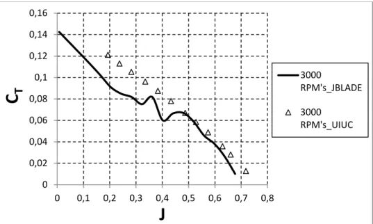
The JBLADE computed propeller performance at 3000 rpm is shown in Figures 3.8, 3.9 and 3.10. The solid lines refer to the simulation and the triangular markers represent the experimental measurements results according to UIUC[13].

Through the graphic in Figure (3.8) it can be seen that the simulation closely follows the measured thrust coefficient performance at high values of the advance ratio, J. For J smaller than 0.45, the simulation falls short on the experimental values, but as J drops below 0.25, the difference is decreasing. For HJ lower than 0.19 there were no measurements. In the static thrust condition, the simulation points to a static thrust coefficient of o.143, close to what one would extrapolate with the experimental data. The oscillations observed in Ct

(41)

21

around J=0.4 can be attributed to lack of convergence in the BEM simulation for some blade elements near 0.75R at such J values. These could not be resolved so far but it is believed that the influence is small far from this critical J value.

Figure 3.8 – APC SF 10x7 calculated versus measured thrust coefficient in function of advance ratio at 3000 RPM.

Figure 3.9 – APC SF 10x7 calculated versus measured power coefficient in function of the advance ratio at 3000 RPM. 0 0,02 0,04 0,06 0,08 0,1 0,12 0,14 0,16 0 0,1 0,2 0,3 0,4 0,5 0,6 0,7 0,8

C

T

J

3000 RPM's_JBLADE 3000 RPM's_UIUC 0 0,01 0,02 0,03 0,04 0,05 0,06 0,07 0,08 0,09 0 0,1 0,2 0,3 0,4 0,5 0,6 0,7 0,8 0,9 1

C

P

J

3000 RPM's_JBLADE 3000 RPM's_UIUC

(42)

22

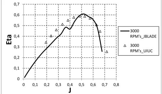
Figure 3.10 - APC SF 10x7 calculated versus measured propeller efficiency in function of the advance ratio at 3000 RPM.

For the power coefficient (see Figure 3.9), the simulation gives close results at low advance ratio and the difference with the experiment increases moderately with J. The highest value of the propeller efficiency is around 61% for the simulations and 59% for the experimental data (JBLADE and UIUC). The advance ratio value for maximum efficiency is also well predicted at J=0.5 as in the real propeller data.

6000 rpm analysis:

The computing process was identical to that executed for the 3000 rpm but with the Reynolds number for this case (see Table 3.2). The JBLADE computed propeller performance at 6000 rpm is shown in Figures 3.11, 3.12 and 3.13. It is seen that apart from the efficiency performance (Figure 3.13), the simulation and the experiment results follow the same trends as in 3000 rpm but is differences are magnified in this case. Again as at 3000 rpm, the maximum efficiency and the maximum efficiency advance ratio are quite close between simulations the experiments.

One important note is that as the as J is reduced, the efficiency difference between JBLADE simulations and the real propeller performance are reduced. This is very important because, in fact, this means that the Ct/Cp ratio prediction is improving at lower J values. Since this Ct/Cp ratio is the critical parameter to optimize in a long endurance propeller for quadcopters, it is concluded that JBLADE is a valid tool for this goal.

0 0,1 0,2 0,3 0,4 0,5 0,6 0,7 0 0,1 0,2 0,3 0,4 0,5 0,6 0,7 0,8

Et

a

J

(43)

23

Figure 3.11 - APC SF 10x7 calculated versus measured validation of calculations: Thrust coefficient versus advance ratio to range of 6000 RPM.

Figure 3.12 - APC SF 10x7 calculated versus measured validation of calculations: power coefficient versus of the advance ratio to range of 6000 RPM.

0 0,02 0,04 0,06 0,08 0,1 0,12 0,14 0,16 0 0,1 0,2 0,3 0,4 0,5 0,6 0,7 0,8 0,9

C

T

J

6000 RPM's_JBLADE 6000 RPM's_UIUC 0 0,01 0,02 0,03 0,04 0,05 0,06 0,07 0,08 0,09 0 0,1 0,2 0,3 0,4 0,5 0,6 0,7 0,8 0,9 1 1,1

C

P

J

(44)

24

Figure 3.13 - APC SF 10x7 calculated versus measured validation of calculations: propeller efficiency versus advance ratio to range of 6000 RPM’s.

A closer look is possible if both simulations 3000rpm and 6000 rpm are drawn in the same graphs. This is shown in Figures 3.14, 3.15 and 3.16. It is observed that the simulations give quite close results at both propeller rotational speeds. On the other hand, the experimental values for Ct and Cp show significant increments when the rotational speed climbs from 3000

to 6000 rpm. Two hypotheses for this behavior can be raised. One is that the Re number increase. The other is that the with the very thin airfoil that this propeller uses, and the designation of slow fly, the blades are prone to deform at higher rotational speed and thrust loadings.

Investigating for the Re number influence hypothesis in the increase in Ct and Cp for the APC

SF 10x7 with rotational speed, the XFOIL simulation results for the propeller airfoil at the corresponding operational Re do not show a significant change in airfoil efficiency between both rotational speeds.

As for the blade deformation hypothesis, all Ct, Cp and  graphs (Figures 3.14, 3.15 and 3.16)

seem to corroborate it since Ct is increased for every J and drops to zero at an increased J as

one would expect for an increased blade pitch, Cp shows the same difference with J as Ct and  maximum is slightly increased but most of all, the maximum efficiency region is extended up to higher J values and the final drop in  is also delay to higher advance ratios as if the propeller pitch would have been increased from the 3000 rpm to the 6000 rpm condition.

0 0,1 0,2 0,3 0,4 0,5 0,6 0,7 0 0,1 0,2 0,3 0,4 0,5 0,6 0,7 0,8 0,9

Et

a

J

(45)

25

Figure 3.14 – Thrust coefficient versus advance ratio to APC SF 10x7.

Figure 3.15 – Power coefficient versus advance ratio to APC SF 10x7. 0 0,02 0,04 0,06 0,08 0,1 0,12 0,14 0,16 0 0,1 0,2 0,3 0,4 0,5 0,6 0,7 0,8 0,9

C

T

J

6000 RPM's_JBLADE 3000 RPM's_JBLADE 3000 RPM's_UIUC 6000 RPM's_UIUC 0 0,01 0,02 0,03 0,04 0,05 0,06 0,07 0,08 0,09 0 0,1 0,2 0,3 0,4 0,5 0,6 0,7 0,8 0,9 1 1,1

C

P

J

6000 RPM's_JBLADE 3000 RPM's_JBLADE 3000 RPM's_UIUC 6000 RPM's_UIUC

(46)

26

Figure 3.16 – Propeller efficiency versus advance ratio to APC SF 10x7.

With evidences that the APC SF 10x7 can be deforming with rotational speed and thrust, this hypothesis deserves further attention. To pay a closer look at this possibility, it should be noted that the APC Slow Flyer is a propeller designed for low RPM’s, so the Reynolds number is not the most influential factor in propeller’s performance as the airfoil has a very low critical Reynolds number.

Figure 3.17 – APC Slow Flyer 10x7. [13]

In order to further reflect on the deformation of the SF propeller hypothesis, two other propellers with dimensions of diameter and pitch very similar to APC 10x7 SF are compared in their performance behavior at different rotational speeds. These are PAC propeller models from different classes of applications expected to have significantly different blade airfoils and structural characteristics.

The first is the APC TE(Thin Electric) 10x7, a propeller designed to allow a given motor to spin as fast as possible for a given propeller diameter. The APC TE propeller family is expected to have a very low Re airfoil as the SF because although expected to rotate faster, the chord is smaller thus the operating Re of the two should be similar.

0 0,1 0,2 0,3 0,4 0,5 0,6 0,7 0 0,1 0,2 0,3 0,4 0,5 0,6 0,7 0,8 0,9

Et

a

J

(47)

27

Figure 3.18 – ACP Thin Electric 10x7. The graphic represents the thrust coefficient versus advance ratio at different rotational speeds. [13]

Figure 3.19– APC Thin Electric 10x7. [13]

Through the curves in the graphic of figure (3.17), it can be seen that although there are changes of the curves Ct with rotational speed at intermediate J values, these are much

smaller that the changes in the SF 10x7. This would be expected because the TE propeller blade is considerably stiffer than the SF mainly because of the bigger airfoil thickness of the TE.

(48)

28

Figure 3.20– ACP Sport 10x8. The graphic represents the thrust coefficient versus advance ratio at different rotational speeds. [13]

Figure 3.21 – APC Sport 10x8. [13]

The second propeller to compare with the SF is the APC Sport 10x8 propeller [13]. It is a very rigid propeller designed for combustion engines with very high rotational speeds compared with the SF and therefore also higher values of Reynolds. When tested by the UIUC team at the same rotational speeds as the SF and TE, it showed considerable differences in the Ct

curves at different rational speeds. Considering that these differences get smaller at higher rotational speeds and that the propeller was spinning at lower than designed rotational speeds, the differences can be attributed to the influence of the Re number in the airfoil performance. Basically, the Sport propeller needs a rotational speed higher than 6000 rpm to make the blade airfoil operate at Re above critical. This could be investigated further if the airfoil was measured and simulated as it was the case for the SF propeller of the validation case.

(49)

29 3.4. Benchmark Propeller

A shorter pitch propeller was found to be more appropriate for the typical quadcopter static thrust operating condition. So APC SF 11x4.7 was analyzed with the assumption that the airfoil would be the same as the APC SF 10x7 model. The validation was not performed directly with the 11x4.7 because the 10x7 was already available at UBI’s laboratory. This propeller was used as the basis for creating a new design for improved quadcopter endurance. As the APC SF 10x7 propeller, the APC SF 11x4.7 was subjected to JBLADE’s analyses for 3000 RPM and 6000 RPM, where UIUC experimental data was available.

Figure 3.6 shows the airfoil and Figure 3.22 describes the SF 11x4.7 blade pitch and incidence distribution.

Figure 3.22 - Propeller incidence and chord distribution for the APC SF 11x4.7 propeller as presented in UIUC Propeller Database [13].

Through the propeller data found in reference [13], it was possible to determine the parameters required for the simulation in JBLADE, similarly to what was done for the APC SF 10x7. Table 3.3 shows the data used to describe the blade in JBLADE and the calculated blade sections operating Reynolds numbers of the propeller at 3000 and 6000 rpm. The Re number calculations as previously were calculated using Equations 3.33 and 3.34.

(50)

30

r/R c/R beta r[m] c[m] _(3000rpm)Re _(6000rpm)Re 0.15 0.112 19.64 0.020955 0.0156464 6971 13942 0.2 0.137 21.81 0.02794 0.0191389 11370 22739 0.25 0.16 22.45 0.034925 0.022352 16598 33196 0.3 0.181 21.88 0.04191 0.0252857 22532 45064 0.35 0.198 20.73 0.048895 0.0276606 28756 57513 0.4 0.211 19.14 0.05588 0.0294767 35022 70044 0.45 0.221 17.3 0.062865 0.0308737 41267 82534 0.5 0.227 15.58 0.06985 0.0317119 47097 94195 0.55 0.23 14.06 0.076835 0.032131 52492 104983 0.6 0.228 12.71 0.08382 0.0318516 56766 113531 0.65 0.222 11.53 0.090805 0.0310134 59878 119756 0.7 0.213 10.47 0.09779 0.0297561 61870 123739 0.75 0.199 9.53 0.104775 0.0278003 61932 123864 0.8 0.181 8.63 0.11176 0.0252857 60085 120171 0.85 0.158 7.71 0.118745 0.0220726 55728 111457 0.9 0.132 6.61 0.12573 0.0184404 49297 98593 0.95 0.084 5.28 0.132715 0.0117348 33113 66227 1 0.035 3.93 0.1397 0.0048895 14523 29047

Table 3.3 - APC 11x4.7 parameters for 3000 RPM and 6000 RPM.

Through the analysis of the propeller in JBLADE together with UIUC data [13], the graphs of Figures 3.23, 3.24 and 3.25 were drawn.

Figure 3.23 – Thrust coefficient versus advance ratio to APC SF 11x4.7. 0 0,02 0,04 0,06 0,08 0,1 0,12 0 0,1 0,2 0,3 0,4 0,5 0,6 0,7

C

T

J

(51)

31

Figure 3.24 – Power coefficient versus advance ratio to APC SF 11x4.7.

Figure 3.25 – Propeller efficiency versus advance ratio to APC SF 11x4.7.

As the propeller APC SF 10x7, the Reynolds number is not expected to have significant influence on propeller’s performance difference between 3000 and 6000 rpm. When subjected to rotation, the 11x4.7 blade seems to be deformed as with the SF 10x4.7. In this case, this effect seems to be so significant that the maximum efficiency value is significantly under predicted at a J value smaller then found in the UIUC experiments. Both these differences between the simulation and the experiments and the differences in the experimental values from 3000 to 6000 rpm are compatible with the blade being deformed to an increased pitch at 3000 and even further to 6000 rpm.

0 0,01 0,02 0,03 0,04 0,05 0,06 0 0,1 0,2 0,3 0,4 0,5 0,6 0,7 0,8

C

P

J

6000 RPM's_JBLADE 6000 RPM's_UIUC 3000 RPM's_JBLADE 3000 RPM's_UIUC 0 0,1 0,2 0,3 0,4 0,5 0,6 0,7 0 0,1 0,2 0,3 0,4 0,5 0,6 0,7

Et

a

J

6000 RPM's_JBLADE 6000 RPM's_UIUC 3000 RPM's_JBLADE 3000 RPM's_UIUC

(52)

32

4. A New Long Endurance Propeller

4.1. Design Concept

The concepts that were implemented to some extent1_{in the new propeller design are:}

a) To adjust pitch to diameter ratio (p/D) such that the propeller is optimized for the static condition.

Comparing the APC’s SF 11x4.7 (SF1) with the SF 11x3.8 (SF2), the experimental static thrust coefficients [13] of both APC’s at 6000 rpm are:

From equation (3.8) the ratio between the SF1 and SF2 thrust coefficients for the same thrust and rpm is:

So, the SF that would replace the SF 11x3.8 would have:

Through the equation (3.7), the required power is determined:

One concludes that the APC SF 11x3.8 (SF2) equivalent, with the same p/D (APC SF 11.8x4.08), that could replace the SF 11x4.7 in a quadcopter while reducing the power consumption by 6.2%.

1_{Not necessarily to the optimum but to the best possible, proximity of optimal or} compromise, with the available time and tools.

(53)

33

Thus, confirming that an adjusted p/D (concept a)) allows a better performance in terms of requered power for a given thrust, thus, a higher endurance for the quadcopter.

b) To increase the diameter (D) for better static thrust efficiency (T/P), without increasing motor load.

According to momentum theory, a static thrust condition will require:

So, the power required for a given thrust will be inversely proportional to the propeller diameter. On the other hand a larger diameter with the same centre of pressure will certainly increase the motor load, i.e. torque. This leads us to c),

c) To taper the blade in chord/lift coefficient such that for the same blade thrust and torque. This will keep the centre of pressure radial position while the blade radius is increased according to a);

Looking at concepts b) and c), the Thin Electric line of APC propellers stands out as a possible alternative to the Slow Fly APC propeller line that we took as a reference for quadcopter use. Comparing the APC SF 11x4.7 with a Thin Electric (TE) Propeller (using data from the TE 11x5.5 as the one with available experimental data by UIUC [13] with the closest p/D to the SF 11x4.7 and assuming that the nondimensional coefficients will not change significantly if the diameter is changed as long as the P/D=5.5/11 is maintained), the following conditions must be imposed:

 The diameter of the TE must be such that the thrust is the same as with the SF 11x4.7 at 6000rpm;

 The static thrust coefficients [13] of both Thin Electric 11x5.5 and Slow Flyer 11x4.7 at 6000 rpm are:

From equation (3.8) the ratio between the SF and TE thrust coefficients for the same thrust and rpm is:

Low reynolds propellers for increased quadcopters endurance

Engenharia