Hydrodynamic profile of young swimmers: Changes over a
competitive season
T. M. Barbosa1,2, J. E. Morais2,3, M. C. Marques2,4, A. J. Silva2,5, D. A. Marinho2,4, Y. H. Kee1 1
National Institute of Education, Nanyang Technological University, Singapore, Singapore,2
Research Centre in Sports, Health and Human Development, Vila Real, Portugal,3
Department of Sport Sciences, Polytechnic Institute of Bragança, Bragança, Portugal, 4
Department of Sport Sciences, University of Beira Interior, Covilhã, Portugal,5
Department of Sport Sciences, Exercise and Health, University of Trás-os-Montes and Alto Douro, Vila Real, Portugal
Corresponding author: Tiago M. Barbosa, PhD, Nanyang Technological University, NIE5-03-32, 1 Nanyang Walk, Singapore 637616, Singapore. Tel: 65 6219 6213, Fax: 65 6896 9260, E-mail: [email protected]
Accepted for publication 28 May 2014
The aim of this study was to analyze the changes in the hydrodynamic profile of young swimmers over a com-petitive season and to compare the variations according to a well-designed training periodization. Twenty-five swimmers (13 boys and 12 girls) were evaluated in (a) October (M1); (b) March (M2); and (c) June (M3). Inertial and anthropometrical measures included body mass, swimmer’s added water mass, height, and trunk transverse surface area. Swimming efficiency was estimated by the speed fluctuation, stroke index, and approximate entropy. Active drag was estimated with the velocity perturbation method and the passive drag with the gliding decay method. Hydrodynamic dimen-sionless numbers (Froude and Reynolds numbers)
and hull velocity (i.e., speed at Froude number= 0.42) were also calculated. No variable presented a significant gender effect. Anthropometrics and inertial parameters plus dimensionless numbers increased over time. Swimming efficiency improved between M1 and M3. There was a trend for both passive and active drag increase from M1 to M2, but being lower at M3 than at M1. Intra-individual changes between evaluation moments suggest high between- and within-subject variations. Therefore, hydrodynamic changes over a season occur in a non-linear fashion way, where the interplay between growth and training periodization explain the unique path flow selected by each young swimmer.
Swimming is a locomotion technique to travel in water. As a land species, humans are not completely adapted to aquatic environments, or at least to the same extent as others. Swimming can be used for purposes of survival, leisure and recreation, health and fitness, and sports and exercise. Performance in swimming is measured by the time spent to cover a given distance. Swimming profi-ciency and performance will depend greatly on the hydrodynamic profile of the subject. The hydrodynamic profile involves analysis of the drag force (passive and active drag), dimensionless numbers (e.g., Reynolds and Froude numbers), and mechanical power and its rela-tionships with anthropometrics, swimming kinematics, and efficiency.
A profile is a collection of features that might charac-terize someone. Sports performance profiling can include anthropometrical, biomechanical, physiological, or psychological variables, among others. Profiling pro-vides athletes with an awareness of their strongest and weak points. Profiling enables a swimmer to excel, as long as the determinant factors of performance are assessed. Swimming performance is a multifactorial phenomenon in which several domains, including
hydrodynamics (Barbosa et al., 2010), play a part. Theo-retical and empirical studies (experimental or numerical simulations) have shown that several hydrodynamic variables are related to performance and/or the competi-tive level. Hydrodynamic profiling may include analysis of the two main streamwise external forces that act upon the swimmer: thrust and drag. Theoretically, swimming velocity is the balance between both forces. To be stricter, the balance between the power output and the drag should provide us the velocity (in m/s):
v P D
= [1]
where v is the velocity (in m/s), P is the power output (in W), and D is the drag, i.e., the resistive force (in N). Confirming theoretical models with empirical data is more challenging. Nevertheless, it has been reported that the three most propulsive phases of the butterfly stroke cycle are the outsweep, the insweep, and the upsweep (Taiar et al., 1999). Improvement in performance is related to power output. Furthermore, hydrodynamic profile shows dramatic changes with training (Toussaint
& Beek, 1992). It has been suggested that, to maximize velocity, drag has to be minimized by tailoring the resis-tance type (friction, pressure, or wave) according to the form of locomotion (e.g., fins swimming vs front crawl stroke) and swim pace (Pendergast et al., 2005). For instance, at speeds below 1 m/s, pressure drag domi-nates, whereas friction drag dominates up to 3 m/s (Pendergast et al., 2005). Swimmers who have recorded the fastest speed also showed the smallest difference in net drag force fluctuations, at least for backstroke (Formosa et al., 2013). Overall, both thrust and drag affect swimming performance.
Thrust is produced from steady and unsteady flows. Steady-flow propulsion is related to the effective propul-sive force (Schleihauf et al., 1988):
Fp=Dprop+ ⋅cosαL [2]
where Fp is the effective propulsive force, Dprop is the propulsive drag, L is the lift force, andα is the absolute angle of the resultant vector in the displacement direc-tion (i.e., horizontal axis). Unsteady-flow propulsion is related to vortex or intermittent jet-flow:
Γ =
∫
ω ds⋅ [3]whereΓ is the vortex circulation, ω is the angular veloc-ity, and ds is the area. The velocity induced by a vortex ring is calculated using Biot–Savart’s law, which can also be applied to hydrodynamics:
v R 0 2 = ⋅ Γ [4] where v0 is the instantaneous induced velocity,Γ is the circulation of vortex ring, and R is the vortex ring radius at a given moment. On the other side, resistance or drag can be calculated with Newton’s equation:
D= ⋅ ⋅ ⋅ ⋅1 v S C 2
2
ρ D [5]
where D is the drag force,ρ is the fluid density, v is the velocity, S is the projection surface, and CD is the drag coefficient. Total drag force includes three components:
D=Df+Dpr+Dw [6] where D is the total drag force, Dfis the friction drag, Dpr is the pressure drag, and Dwis the wave drag. The total drag or each one of its components can be measured when the swimmer glides or is towed with no segmental action (i.e., passive drag) or he propels himself (i.e., active drag). Dfis attributed to tangential forces that slow down the water flowing around the body surface. Dpris caused by the pressure differential between the front and the rear parts of the body. Both Dfand Dprare strongly related to the fluid flow around the body. The Reynolds number (Re) is a dimensionless variable expressing the
ratio between inertial and viscous forces, hence quanti-fying the flow conditions. Dwis due to the displacement of the body at surface, which catches and compresses fluid, setting up a wave system. With increasing depth the effect of Dw decreases meaningfully, i.e., there is a significant and moderate/large effect size, hence making it a relevant phenomenon for swimming (Vorontsov & Rumyantsev, 2000). Experimental evidence suggests that Dwcan be neglected when a swimmer is fully sub-merged (Naemi et al., 2010). Froude number (Fr) and hull velocity (vhull) can be used complimentarily to assess wave resistance (Kjendlie & Stallman, 2008). The Froude number represents the ratio of inertial to gravi-tational forces experienced by a body moving at or close to a fluid/fluid interface (Webb, 1975). Therefore, wave-making resistance is related to Fr, whereas vhull is the critical velocity where upon the wave wake length is equal to hull length. The Dwincrease is less sharp above
Fr= 0.45 (Vennell et al., 2006). At Fr = 0.42, the body is
trapped in the hull, moving along with the wave system, i.e., the vhull (Vogel, 1994), and therefore is more eco-nomic and efficient. Comparing adults and children, the former present a higher maximal swim speed, but also Fr and Re (Kjendlie & Stallman, 2008). Besides that, per-formance enhancement was coupled with increases in Fr and Re (Toussaint et al., 1990).
Because it is so challenging to directly measure swim-ming efficiency, researchers tend to select a few estima-tors. These estimators are based on the reasoning that, according to Newton’s laws, resistance to any change in a body motion will increase the energy demand. Higher variations in the state of the motion (i.e., velocity changes) likewise will increase the energy cost of trans-portation. Speed fluctuation and stroke index are two variables most cited in the swimming literature (Barbosa et al., 2010). In young swimmers, it was reported that as speed increases, speed fluctuation tends to decrease (Barbosa et al., 2012) and stroke index tends to increase (Latt et al., 2009). However, claims that both parameters are not sensitive or informative enough have been increasing. This might be due to the fact that both param-eters assess intra-cyclic variations, i.e., changes in a very short period of time. There is always a delay between the start of a physical effort and the neuromuscular, kine-matic, and kinetic and energetic acute responses. Whereas kinematic changes take no longer than a few tenths of a second to happen, the kinetic and energetic response to such changes might need some seconds or minutes. Hence, a parameter that allows assessment of the speed inter-cyclic changes throughout several stroke cycles can be a true novelty and deliver more insightful details.
Approximate entropy (ApEn; Pincus, 1991) is one non-linear technique used to quantify the regularity of fluctuations over time series data. In this regard, ApEn might allow us to learn about the inter-cyclic variations of the horizontal velocity. According to the published
literature, this measure has not been used previously to assess competitive swimming or any other competitive technique. However, it has been used in other fields, for instance, to assess body sway (e.g., Kee et al., 2012), gait analysis of patients (e.g., Arif et al., 2004), and nota-tional analysis in team sports (Sampaio & Maçãs, 2012). Several methods have been reported for hydrody-namic testing. Active drag can be assessed using ener-getic procedures, the velocity perturbation method (VPM), the assisted towing method (ATM), the measur-ing active drag system (MAD), and computer fluid dynamics (CFD) (Havriluk, 2007; Barbosa et al., 2013; Formosa et al., 2013). Passive drag can be assessed using the glide decay method, the isokinetic engine or strain gauge while being towed, the ATM, and computational fluid dynamics (Havriluk, 2007; Barbosa et al., 2013). Some of these methods involve the measurement before-hand of inertial and kinematic data. After anthropometric [i.e., inertial parameters, such as body mass (BM) or added water mass] and kinematic (i.e., speed and accel-erations) data are collected, drag force is calculated according to Newton’s law of motion and Newton’s law of resistance. To estimate efficiency, kinematic data may be collected using mechanical speedometers, motion capture systems, and, more recently, inertial measure-ment units tracking the head, hip, or center of mass (Barbosa et al., 2012). Because of the large variety of procedures available, comparison of data across different papers is very challenging, as all methods have advan-tages and disadvanadvan-tages. Not one procedure is consid-ered by the scientific community as a true gold standard, at least for hydrodynamic testing.
Evidence on hydrodynamic changes over time in young and even adult swimmers is scarce. After an 8-week preparation to build up aerobic capacity and aerobic power and to enhance swimming technique of young swimmers, there were no significant changes in active drag or coefficient of active drag assessed with the VPM (Marinho et al., 2010). Surprisingly, 1 week of instructional intervention (including swim drills with specific visual and kinesthetic cues) was enough to decrease the coefficient of active drag, mea-sured with a barometric technique, in pubescent coun-terparts (Havriluk, 2006). Training programs focused on energetic buildup might probably not affect hydrody-namics; however, if the objective is to improve tech-nique, such programs might have an effect, even in a short time frame. Nevertheless, further research should be carried out to clarify the relationship between differ-ent training programs and the hydrodynamic profile. Indeed, it is suggested that a complex process takes place in the interplay between growth, technique, and hydro-dynamics, which for this case was measured on the MAD system (Toussaint et al., 1990), even though some care should be exercised in interpreting these findings, as the MAD system imposes a few constraints compared with free swimming, especially in children. A broad and
holistic approach, reporting both passive and active drag plus swimming efficiency, has never been done before, as much as we are aware of. Indeed most of the scarce literature focuses on active drag (i.e., clean swimming). However, top performance in major international com-petitions suggests that starts and turns are key moments of a race. As such, a renewed interest has emerged for the passive drag (i.e., gliding after the start and each turn). On top of that, new trends in sports science and coaching strongly suggest that longitudinal designs should monitor training loads, as this might be a confounding factor (Mujika, 2013). Unfortunately, the literature avail-able does not provide detailed reports of the training loads.
The current study aimed to analyze the changes in the hydrodynamic profile of young swimmers over a com-petitive season and compare the variations of this profile according to training periodization. It was hypothesized that if training planning is designed with two major macro-cycles (one general preparation cycle to build up energetic and the other more specific on the road to the main competition), the hydrodynamic profile would be impaired in the first macro-cycle and enhanced in the second.
Methods
Subjects
Twenty-five talented swimmers were assessed (13 boys: 12.64± 0.81 years old and 68.02 ± 5.49 s personal best in short-course swimming pool at freestyle; 12 girls: 12.43± 0.78 years old and 71.23± 5.45 s personal best; both genders in Tanner stages 1–2 by self-report at the beginning of the research). The sample included age group national record holders, age group national champions, and other swimmers who are part of a national talent identification and follow-up project.
Coaches, parents, and/or guardians and the athletes gave informed consent for participation in this study. All procedures were in accordance with the Declaration of Helsinki regarding human research. The University Ethics Board also approved the research design.
Study design
A longitudinal research design was selected, including repeated measures of several hydrodynamic variables in three different moments (Mi) over one season. Swimmers were evaluated in the following periods: (a) October (M1, the season’s first competi-tion); (b) March (M2, the winter’s peak competicompeti-tion); and (c) June (M3, the summer’s peak competition). Between October and Feb-ruary, the training program had, as its major goal, to build up energetics, being characterized by a fairly high volume (Table 1). Between March and June the main goal was to fine-tune technique and build up energetics at race pace on the road to the major competition of the season (Table 1). Data collection procedures were carried out under the same testing conditions at all times (e.g., the same swimming pool, time of day, lane, no other swimmer was in the lane or nearby lanes to reduce drafting and pacing effects, affecting the drag force).
A potential confounding factor for the analysis of the changes over time was the intra-subject variability within a testing session and between testing sessions. True/meaningful changes do occur
when intra-subject variability over time (i.e., between testing ses-sions) is higher than that verified in a single moment (i.e., within a testing session, performing several trials of the same task). Vantorre et al. (2010) analyzed the variability of front crawl starts in elite (89.3%± 3.0% of the 100 freestyle World Record) and trained swimmers (79.9%± 8.0% of the World Record). The start was split into several phases, including the “swimming phase” (i.e., the time from the beginning of the first arm stroke to the instant the head reached the 15-m mark), which can be selected to learn about the intra-subject variability. Examination of intertrial variability revealed high reproducibility for the swimming phase (ICC= 0.951 for trained; ICC = 0.981 for elite swimmers). Earlier data not published from our research group suggest an intra-subject variability of 11% for passive drag and 9% for stroke kinematics in young swimmers. Therefore, a true/meaningful change over time if variability is higher than 10% is expected.
Anthropometrics and inertial parameters
BM was measured with a digital weight scale (SECA, 884, Hamburg, Germany) (ICC= 0.99). The swimmer’s added water mass (ma) was estimated as being approximately 27% [26.8%± 2.3%, mean ± standard error (SE)] for a subject with similar age (Caspersen et al., 2010). Height was measured with a digital stadiometer (SECA, 242, Hamburg, Germany) on the upright position, barefoot, and in swimwear (ICC= 0.99). All anthropometric measurements were collected according to stan-dardized procedures.
The trunk transverse surface area (TTSA) was measured with a photogrammetric technique (Morais et al., 2011). Swimmers were photographed with a digital camera (DSC-T7, Sony, Tokyo, Japan) in the transverse plane from above (Caspersen et al., 2010). Sub-jects stood on land, on the upright, and streamlined position. This position is characterized by having the arms fully extended above the head, one hand over the other, fingers also extended close together, and head in neutral position. Subjects wore a regular textile swim suit, cap, and goggles. On the camera shooting field, a calibration frame with 0.945 m in length was aside the swimmer at the shoulders level. The TTSA was measured with an area measuring software (Udruler, AVPSoft, USA) after importing the digital picture (ICC= 0.97).
Kinematics and non-linear parameter
Each swimmer performed a maximal 25-m front crawl trial with a push-off start. Because data were collected in a short-course swim-ming pool, subjects were advised to reduce gliding during the start so that it would be possible to collect data between the 11th and
the 24th meter. A speedometer cable (Swim speedometer, Swimsportec, Hildesheim, Germany) was attached to the swim-mer’s hip (Barbosa et al., 2012). The speedometer was placed on the forehead wall of the swimming pool, about 0.2 m above water surface. A software’s interface in LabVIEW® (v. 2009, National Instruments, Austin, TX, USA) was used to acquire (f= 50Hz), display, and process speed– time data online during the trial. Data were transferred from the speedometer to the software application with a 12-bit resolution acquisition card (USB-6008, National Instruments, Austin, Texas, USA). Although the speedometer is a “coach-friendly” piece of equipment (it is affordable, easy to operate, and it allows immediate feedback for swimmer), the hip’s
dv does not represent with total accuracy the center of the mass’s dv. Two major sources of error should be acknowledged: (a)
speedometer measures the speed of a fixed point and (b) inertial effects might act upon the system. A 0.1-s time delay (i.e.,∼10% of the stroke cycle duration), a 0.2 m/s higher speed range (i.e., less than 10% of the maximal speed for young swimmers), and a moderate root mean square (RMS) error (0.16≤ RMSerror≤ 0.3) comparing hip and center of mass kinematics at front crawl (Figueiredo et al., 2009; Psycharakis & Sanders, 2009) have been reported. Comparing hip speed collected with speedometer and a motion capture system, there is a 0.002± 0.001 difference [mean± SE, standard deviation (SD) = 0.012, −0.001; 0.005 for a 95% confidence interval] at front crawl and backstroke for swim-mers with similar age and competitive level of our subject (Feitosa et al., 2013). Whenever any problems were identified through visual observation/inspection of curves, the swimmers were asked to repeat the trial. This was by no means expected to eliminate every problem that might have occurred through testing (e.g., bumping feet on the cable). Rather, it was used as an extra pre-caution to exclude problematic trials.
Thereafter, data were exported to a signal processing software (AcqKnowledge v. 3.9.0, Biopac Systems, Santa Barbara, Califor-nia, USA) and filtered with a 5-Hz, cut-off, low-pass fourth-order Butterworth filter according to the analysis of the residual error vs cut-off frequency output. The intra-cyclic variation of the horizon-tal velocity of the hip (dv) was analyzed (Barbosa et al., 2010):
dv v v F n v F n i i = − ⋅
∑
∑
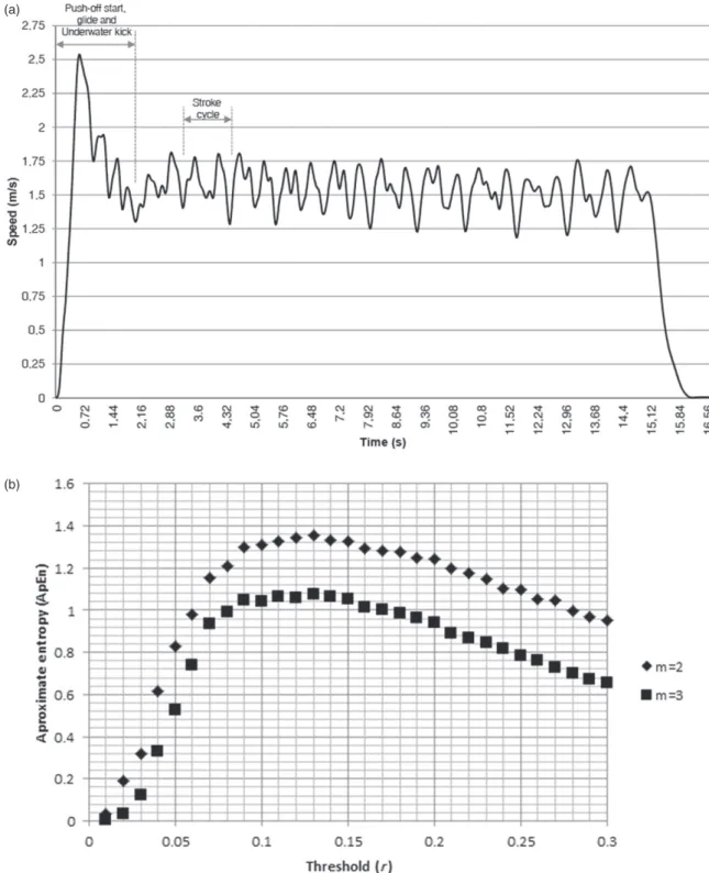
( i ) i i i 2 100 . . [7]where dv represents the intra-cyclic variation of the horizontal velocity of the hip, v represents the mean swimming velocity, vi represents the instant swimming velocity, Firepresents the acqui-sition frequency, and n is the number speed–time pairs. For further analysis, the dv mean values of three consecutive stroke cycles between the 11th and 24th meter from the starting wall were considered (Fig. 1(a)).
The stroke index, as an overall swimming efficiency estimator, was calculated (Costill et al., 1985):
SI=SL v⋅ [8]
where SI is the stroke index, SL is the stroke length, and v is the swimming velocity. The SL was calculated from the v and SF collected with the speedometer:
SL v SF
= [9]
where SL is the stroke length, v is the swimming velocity, and SF is the stroke frequency.
The ApEn is a non-linear technique to quantify the temporal structure of (un)predictability in its fluctuations over a given time
Table 1. Total external training loads
October–February (M1–M2) March–June (M2–M3) Volume (km) 497 481 Training sessions 117 114 A0 (km) 209.5 197.5 A1 (km) 189.1 156.7 A2 (km) 55.7 58.7 A3 (km) 20.6 21.7 LT (km) 4.3 4.4 LP (km) 2.7 2.5 RP (km) 1.5 3.8 Sprint (km) 9.1 8.4
A0, warm-up and cool-down; A1, low aerobic capacity; A2, anaerobic threshold; A3, aerobic power; LP, lactate power; LT, lactate tolerance; RP, race pace.
series data. Hence, it can be used to assess the inter-cyclic variation of the horizontal velocity of the hip. It ranges from 0 to 2. A low
ApEn value indicates that the time series is deterministic, and a high
value indicates randomness. The ApEn is derived based on the following algorithm (Pincus, 1991; Pincus & Goldberger, 1994):
ApEn N m r C r C r ( , , ) ln ( ) ( ) = ⎡ ⎣⎢ ⎤ ⎦⎥ + m m 1 [10] where ApEn is the approximate entropy, N is the data length (N= 700 speed–time pairs, according to the suggestion of Yentes
et al., 2013), m is the embedding dimension (m= 2, because two consecutive cycles contributing to two data points were considered for each mobile window), r is the tolerance value or similarity criterion (r= 0.1, determined beforehand as the maximum ApEn for a wide range of r values between 0.01 and 0.3 as suggested by Chon et al., 2009 and Yentes et al., 2013), and
C r n N m im im ( )= − +1 [11]
where Cimis the fraction of patterns of length, nimis the number of patterns that are similar between two sets (given the similarity
(a)
(b)
Fig. 1. Example of the speed fluctuation during one trial (a) and approximate entropy (ApEn) variations for a range of tolerance values
criterion, r), N is the data length, and m is the embedding dimen-sion. It should be highlighted that the selection of different input values can be a potential source of error. Changes in the m and/or
r have an influence on the ApEn (Fig. 1(b)).
Active drag
The VPM was used to estimate active drag (Kolmogorov & Duplischeva, 1992). Active drag was calculated from the differ-ence between the swimming velocities with and without towing a perturbation buoy. To ensure similar maximal power output of both sprints, the subjects were instructed to swim front crawl at maximal pace after a push-off start. Swimming velocity (vertex as reference) was measured for 13 m (between 11th and 24th of the starting wall) with a stopwatch (Golfinho Sports MC-815, Aveiro, Portugal) by two expert evaluators, and the mean value was used for further analysis (ICC= 0.96). Active drag (Da) was calculated as (Kolmogorov & Duplischeva, 1992):
D D v v v v a b b b = ⋅ ⋅ − 2 3 3 [12]
where Darepresents the swimmer’s active drag at maximal veloc-ity, Dbis the resistance of the perturbation buoy provided by the manufacturer, and vband v are the swimming velocities with and without the perturbation device, respectively. The active drag coef-ficient (CDa) was calculated as:
C D S v Da a = ⋅ ⋅ ⋅ 2 2 ρ [13]
whereρ is the density of the water (being 1000 kg/m3), D ais the active drag, v is the swimming velocity, and S is the swimmer’s projected frontal surface area (or TTSA; see “Anthropometrics and inertial parameters” subsection). The power needed to overcome the drag force (PD) was computed as:
PD=D va⋅ [14]
where PDis the power to overcome drag force, Dais the active drag, and v is the swimming velocity.
Passive drag
The passive drag was assessed with inverse dynamics of the gliding decay speed (Klauck & Daniel, 1976). Swimmers were instructed to perform a maximal push-off on the wall fully immersed, at a self-selected depth, ranging approximately between 0.5 and 1.0 m to avoid Dw(Vorontsov & Rumyantsev, 2000). Gliding was performed in the streamlined gliding position (head in neutral position, looking at the bottom of the swimming pool, legs fully extended and close together, arms fully extended at the front, and with one hand over the other) with no segmental actions. Testing ended when swimmers broke the surface and/or were not able to make any further horizontal displacement gliding and/or started any limbs’ actions.
A speedometer cable (Swim speedometer, Swimsportec) was attached to the swimmer’s hip, and the gliding velocity decay was acquired online (f= 50 Hz) (Barbosa et al., 2013). Data were exported to a signal processing software (AcqKnowledge v. 3.9.0, Biopac Systems) and filtered with a 5-Hz, cut-off, low-pass fourth-order Butterworth filter.
The gliding mean velocity and the corresponding mean accel-eration based on the accelaccel-eration to time were calculated with moving time frame windows. The acceleration to time curve was obtained by numerical differentiation of the filtered speed–time curve, using the fifth-order centered equation (Vilas-Boas et al., 2010): a v v v v t i i i i i =2 − −16 − +16 + −2 + 24 2 1 1 2 Δ [15]
where ai is the hip’s instantaneous acceleration, vi is the hip’s instantaneous velocity, and t is the time. Passive drag (Dp) force was calculated as:
Dp=(BM+ma)⋅a [16]
where Dpis the passive drag, BM is the swimmers on-the-day BM, mais the swimmer’s added water mass, and a is the acceleration. The passive drag coefficient (CDp) was calculated as:
C D S v Dp p = ⋅ ⋅ ⋅ 2 2 ρ [17]
whereρ is the density of the water (being 1000 kg/m3), D pis the passive drag, v is the gliding velocity, and S is the projected frontal surface area. The total drag index (TDI) was assessed as a hydro-dynamic efficiency estimation (Kjendlie & Stallman, 2008). To learn if the swimmer relies more on the Daor Dp(Kolmogorov & Duplischeva, 1992): TDI D D = a p [18] where TDI is the drag technique index, Dais the active drag, and Dpis the passive drag.
Froude number, hull speed, and Reynolds number
The Froude number is a dimensionless parameter that is consid-ered as a wave-making resistance index (Kjendlie & Stallman, 2008):
Fr v g H
=
⋅ [19]
where v is the swimming velocity (collected with the speedom-eter), g is the gravitational acceleration, and H the swimmer’s height. Hull velocity, i.e., the speed at a Froude number equal to 0.42 (Vogel, 1994), was also selected:
vh= g H
⋅ ⋅
2 π [20]
where g is the gravitational acceleration and H is the height. The Reynolds number was used to assess the water flow status sur-rounding the swimmer:
Re= ⋅v H
υ [21]
where v is the swimming velocity, H is the height, andυ is the water kinematic viscosity (being 8.97× 10⁻⁷m2/s at 26 °C). Statistical procedures
The homoscedasticity assumption was checked with the Levene test. Normality [defined as Y∩N (μY|X1,X2, . . . ,XK,σ2)] was deter-mined with the Shapiro–Wilk test. Mean± 1 SD is reported for all variables.
Data variation was analyzed with two-way analysis of variance (ANOVA) (time effect, gender effect, time× gender interaction) followed by the Bonferroni post-hoc test (P≤ 0.05), whenever suitable. Total eta square (η2) was selected as effect size index and interpreted as (a) no effect if 0< η2≤ 0.04; (b) minimum if 0.04< η2≤ 0.25; (c) moderate if 0.25 < η2≤ 0.64; and (d) strong if η2> 0.64.
For each evaluation moment, after the diagnosis of multicolinearity effects (including independence of the measures), correlation coefficients were calculated (P≤ 0.05). As rule of thumb the following were considered: (a) small effect size if 0≤ |R| ≤ 0.2; (b) moderate effect size if 0.2 < |R| ≤ 0.5; and (c) strong effect size if |R|> 0.5.
Results
No variables presented a significant gender effect (Table 2). All selected variables but dv, Dp, and CDp presented a time effect (Table 2; Figs. 1–4). Anthropometrics and inertial parameters increased over time (Table 2; Fig. 2). ApEn and SI suggest that swim-ming efficiency improved (Table 1; Fig. 3). Da, CDa, PD, and TDI increased at M2 but then decreased at M3 to values lower than observed at baseline (Table 2; Fig. 4). There was a non-significant decrease of CDp over time. Dimensionless numbers increased from M1 to M3 (Table 2; Fig. 5). Overall, it seems that the changes occurred in a non-linear fashion way. The effect size index suggests a minimum-to-strong effect size for the
variables with significant effects (0.21≤ η2≤ 0.75). Nine of the 11 variables are within the “moderate” band though. Only the height and the vhullshowed significant time× gender interactions but with no effect (Table 2).
Intra-individual changes between evaluation moments suggest a high between- and within-subject variation (Table 3). The variables related to drag, such as Da, Dp, and therefore, CDa, CDp, PD, and TDI, have the highest within-subject changes. Between-subject changes can be analyzed with the SD. Once again, variables related to passive and active drag plus dv have the highest varia-tions. Variables related to anthropometrics and inertia, swimming efficiency, and dimensionless numbers had a lower intra-individual change.
For a set of computed correlations, the odds of some being significant will be only by chance. With signifi-cance accepted at P< 0.05, for every 20 correlations performed, on average one might be significant by chance. Correlations were computed between all vari-ables in the three evaluation moments (3 moments× 15 variables× 15 variables). To minimize the odds of type I
Table 2. Data variation (two-way ANOVA) for the selected variables over one season (time effect) for boys and girls (gender effect)
Time effect d.f. (2,46) Eta2 Gender effect d.f. (1,23) Eta2 Time× gender interaction d.f. (2,46) Eta2
F P F P F P BM (kg) 70.768 < 0.001 0.49 0.781 0.39 0.03 2.221 0.48 0.02 H (cm) 61.778 < 0.001 0.69 1.959 0.18 0.08 5.220 0.01 0.06 TTSA (m2) 6.267 0.01 0.21 0.545 0.47 0.02 0.082 0.92 0.01 dv (dimensionless) 2.366 0.10 0.07 0.167 0.69 0.01 0.518 0.60 0.01 ApEn (dimensionless) 10.893 < 0.001 0.31 0.166 0.69 0.01 1.674 0.19 0.04 Da(N) 15.296 < 0.001 0.39 0.563 0.46 0.02 0.511 0.60 0.01 CDa(dimensionless) 12.688 0.47 0.28 1.150 0.30 0.05 0.782 0.46 0.02 Dp(N) 0.773 0.47 0.03 0.447 0.51 0.02 0.703 0.50 0.03 CDp(dimensionless) 0.763 < 0.001 0.03 0.186 0.67 0.01 0.155 0.84 0.01 PD(W) 15.884 < 0.001 0.40 0.967 0.34 0.04 0.744 0.48 0.02 TDI (dimensionless) 10.042 < 0.001 0.30 0.060 0.70 0.01 0.935 0.41 0.03 SI (m2/s) 15.501 < 0.001 0.38 0.162 0.69 0.01 2.342 0.11 0.06 Fr (dimensionless) 13.382 < 0.001 0.38 2.392 0.14 0.11 0.915 0.41 0.01 vhull(m/s) 49.177 < 0.001 0.75 1.643 0.21 0.07 5.017 0.01 0.01 Re (dimensionless) 39.236 < 0.001 0.60 3.231 0.08 0.12 3.174 0.06 0.05
ANOVA, analysis of variance; ApEn, approximate entropy; BM, body mass; CDa, coefficient of active drag; CDp, coefficient of passive drag coefficient; Da,
active drag; d.f., degrees of freedom; Dp, passive drag; dv, speed fluctuation; Fr, Froude number; H, height; PD, mechanical power to overcome drag; Re,
Reynolds number; SI, stroke index; TDI, total drag index; TTSA, trunk transverse surface area; vhull, hull velocity.
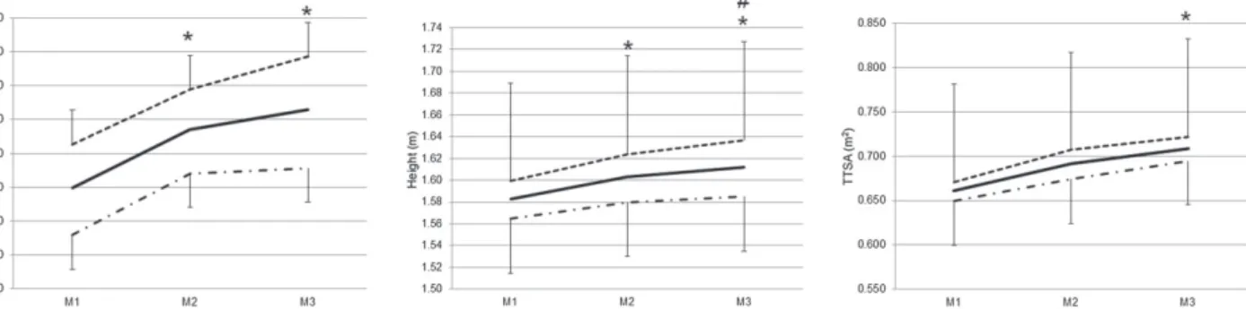
Fig. 2. Changes in anthropometrics and inertial parameters. Solid line (—) overall sample; dash line (- - -) boys; dash and dotted line
(-.-.-) girls; *Post-hoc test between M1 and M2 or M1 and M3 (P≤ 0.05); #Post-hoc test between M2 and M3 (P ≤ 0.05). TTSA, trunk transverse surface area.
error, only the correlation between independent variables is reported. On top of that, an effect size index was selected (cf. “Statistical procedures” subsection). At M1,
Daand PDhad significant and moderate correlations with
Fr (R= 0.41, P = 0.02; R = 0.50, P = 0.01), vhull (R= 0.35, P = 0.04; R = 0.42, P = 0.02), and Re (R= 0.41, P = 0.02; R = 0.52, P = 0.01). SI was strongly associated with Fr (R= 0.65, P < 0.001), vhull(R= 0.62, Fig. 3. Changes in kinematic and non-linear parameters. Solid line (—) overall sample; dash line (- - -) boys; dash and dotted line
(-.-.-) girls; *Post-hoc test between M1 and M2 or M1 and M3 (P≤ 0.05); #Post-hoc test between M2 and M3 (P ≤ 0.05). ApEn, approximate entropy; dv, speed fluctuation; SI, stroke index.
Fig. 4. Changes in drag force. Solid line (—) overall sample; dash line (- - -) boys; dash and dotted line (-.-.-) girls; *Post-hoc test
between M1 and M2 or M1 and M3 (P≤ 0.05); #Post-hoc test between M2 and M3 (P ≤ 0.05). CDa, coefficient of active drag; CDp, coefficient of passive drag coefficient; Da, active drag; Dp, passive drag; PD, Mechanical power to overcome drag; TDI, total drag index.
Fig. 5. Changes in Froude number, hull speed, and Reynolds number. Solid line (—) overall sample; dash line (- - -) boys; dash and
dotted line (-.-.-) girls; *Post-hoc test between M1 and M2 or M1 and M3 (P≤ 0.05); #Post-hoc test between M2 and M3 (P ≤ 0.05).
P< 0.001), and Re (R = 0.75, P < 0.001). TTSA was
strongly associated with SI (R= 0.58, P < 0.001), vhull (R= 0.72, P < 0.001), and Re (R = 0.61, P < 0.001).
At M2, PDwas correlated with SI (R= 0.48, P = 0.01),
Fr (R= 0.42, P = 0.02), vhull(R= 0.52, P = 0.01), and Re (R= 0.59, P < 0.001). Dp had a moderate association with vhull (R= 0.38, P = 0.03) and Re (R = 0.36,
P= 0.04), dv with TDI (R = −0.35, P = 0.04), but SI
cor-related strongly with vhull (R= 0.68, P < 0.001) and Re (R= 0.85, P < 0.001).
Finally, at M3 Da was related to Dp (R= 0.62,
P< 0.001), Fr (R = 0.60, P < 0.001), vhull (R= 0.39,
P= 0.02), and Re (R = 0.57, P = 0.01). A similar trend
was observed for the relationships between PD and Dp (R= 0.63, P < 0.001), SI (R = 0.35, P = 0.04), Fr (R= 0.66, P < 0.001), vhull (R= 0.45, P = 0.01), and
Re (R= 0.63, P < 0.001). Besides that, Dpwas correlated with SI (R= 0.47, P = 0.01), Fr (R = 0.47, P = 0.01), vhull (R= 0.50, P < 0.001), and Re (R = 0.56, P < 0.001).
Discussion
This study aimed (a) to analyze the changes in the hydro-dynamic profile of young swimmers over a season and (b) to assess the changes in the hydrodynamic profile according to the periodization designed. Hydrodynamic changes occurred in a non-linear fashion way. Some of the individual changes observed were affected by factors such as growth and periodization. The general prepara-tion cycle, at the beginning of the season, had a higher focus on the energetic buildup, and the hydrodynamics profile was impaired. Meanwhile, the hydrodynamics profile was enhanced significantly after the specific preparation cycle (aiming to fine-tune technique and
build up energetics at race pace) on the road to the major competition of the season.
No variables presented a significant gender effect, and a couple had a significant time× gender interactions but with no effect (Table 2). There is a very solid body of knowledge that no gender gap exists before puberty. This was already reported by several empirical papers on swimming kinematics, efficiency, anthropometrics, and performance, as reviewed elsewhere (Seifert et al., 2010). In this sense, data might be analyzed either by gender or pooled sample. As for hydrodynamics, one paper revealed significant differences in Da, Dp, and related outcomes, but for pubertal boys and girls (Barbosa et al., 2013). To the best of our knowledge, no study compares the hydrodynamics between genders at such earlier ages and/or maturational state. Even so, however, hydrodynamics depends mostly on anthropometrics and kinematics. Because there is no gender gap before puberty in both domains, it is expected that the same would happen for hydrodynamic outcomes.
It is no surprise that anthropometrics and inertial parameters increased over time (Table 2; Fig. 1). Chil-dren experience physical changes as part of their biologi-cal development (Malina & Bouchard, 1991), including young swimmers that others have reported as having similar percentage of change to the ones verified in this research (Toussaint et al., 1990; Latt et al., 2009). The three swimming efficiency estimators suggest that there is an improvement in such outcomes over time, notably between M2 and M3 (i.e., the cycle with a higher focus on technique enhancement) (Fig. 2). ApEn and SI showed a significant improvement between M1 and M3. However, dv presented a non-significant decrease. For the changes over time smaller than 10%, the variation might as well be related to intra-swimmer variability as explained earlier in the Methods section (cf. “Study design” subsection).
SI is a classical outcome to roughly estimate overall
swimming efficiency. The pioneering paper by Costill et al. (1985), which describes and validates SI, is among the highest cited papers in “swimming science.” The bibliometric data reveal how much the swimming com-munity recognizes SI as a good approximation of overall swimming efficiency. The SI of at least adult national-and international-level swimmers increases slightly throughout a season (Costa et al., 2012). Over two con-secutive seasons, sub-elite swimmers might increase SI around 4% (Costa et al., 2013). Latt et al. (2009) reported an improvement of SI over time for young swimmers as well. Others did not report SI directly, but based on SL and v, one might consider that SI also increased throughout time (e.g., Wakayoshi et al., 1993; Anderson et al., 2006), although it is a rough estimator that does not provide insight about detailed energy path flow from input (as metabolic energy) all the way up to output (as external mechanical work).
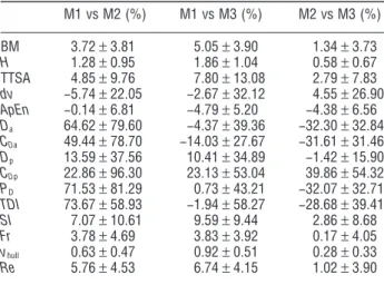
Table 3. Intra-individual changes (%) between evaluation moments
M1 vs M2 (%) M1 vs M3 (%) M2 vs M3 (%) BM 3.72± 3.81 5.05± 3.90 1.34± 3.73 H 1.28± 0.95 1.86± 1.04 0.58± 0.67 TTSA 4.85± 9.76 7.80± 13.08 2.79± 7.83 dv −5.74± 22.05 −2.67± 32.12 4.55± 26.90 ApEn −0.14± 6.81 −4.79± 5.20 −4.38± 6.56 Da 64.62± 79.60 −4.37± 39.36 −32.30± 32.84 CDa 49.44± 78.70 −14.03± 27.67 −31.61± 31.46 Dp 13.59± 37.56 10.41± 34.89 −1.42± 15.90 CDp 22.86± 96.30 23.13± 53.04 39.86± 54.32 PD 71.53± 81.29 0.73± 43.21 −32.07± 32.71 TDI 73.67± 58.93 −1.94± 58.27 −28.68± 39.41 SI 7.07± 10.61 9.59± 9.44 2.86± 8.68 Fr 3.78± 4.69 3.83± 3.92 0.17± 4.05 vhull 0.63± 0.47 0.92± 0.51 0.28± 0.33 Re 5.76± 4.53 6.74± 4.15 1.02± 3.90
ApEn, approximate entropy; BM, body mass; CDa, coefficient of active drag; CDp, coefficient of passive drag coefficient; Da, active drag; Dp,
passive drag; dv, speed fluctuation; Fr, Froude number; H, height; PD,
mechanical power to overcome drag; Re, Reynolds number; SI, stroke index; TDI, total drag index; TTSA, trunk transverse surface area; vhull, hull
The dv was first introduced as an estimation of swimming efficiency for butterfly and breaststroke (e.g., Barbosa et al., 2005). The main assumption is that intra-cyclic changes will impose a higher energy demand and therefore a lower efficiency. There are some claims that intra-cyclic variations might not be sensitive enough to small changes in the swim pace or given swimming strokes where dv has a fairly low range (e.g., front crawl and backstroke). For instance, unless an incremental and maximal protocol is imple-mented it seems that the changes in dv are quite low. Even so, most of the time the protocols include a very narrow pace range (Greco et al., 2013). A second expla-nation for the lower sensitivity is that, according to some determinist models, dv is an intermediate variable between the energetic and biomechanical fields, depending on third-party variables. A few papers have reported that the dv is consistent within adult swim-mers for different velocities (e.g., Schnitzler et al., 2008; Psycharakis et al., 2010). It seems, however, that there is no paper reporting the change of dv over time for either young or adult swimmers. In this sense, dv is the balance of several determinant factors, and each one can play a major or minor role in dv depending on the imposed constrains (task, environment, and organ-ismic) at each moment.
The second explanation leads us to address move-ment variability. For a long time a lower variability was considered as noise that should be minimized or eradi-cated to enable high performance levels (Davids et al., 2004). However, research in ecological dynamics sug-gested that movement variability should not necessarily be construed as noise, which is detrimental to perfor-mance (Davids et al., 2004). Evidence on this was also obtained for swimming (e.g., Komar et al., 2013). To this end, we explored the use of ApEn in assessing the inter-cycle changes, given its potential utility for quan-tifying the structure of temporal variability. Indeed, the selection of non-linear parameters, such as ApEn, is a step forward in this research field. ApEn has been used in the analysis of time series data in biomechanics, most notably in postural balance (e.g., Kee et al., 2012) and gait analysis (e.g., Arif et al., 2004). Conceptually,
ApEn quantifies the probability of predetermined length
of consecutive data segments repeating with other seg-ments of the same length within the same time series data. ApEn is a dimensionless measure that ranges from 0 (signifying repeatability) to 2 (signifying random-ness) (Pincus, 1991; Cavanaugh et al., 2007). ApEn quantifies the temporal structure of predictability of time series data. Based on the dynamical systems per-spective of motor control, heightened systems com-plexity is indicative of adaptive control of degrees of freedom in the movement system. Because ApEn has never been used before in the analysis of competitive swimming, and the algorithm is presumably suited for small data sets of between 50 and 5000 data points
(Stergiou et al., 2004), the use of ApEn could allow us to learn about the inter-cyclic variations of the horizon-tal velocity from a fresh perspective. ApEn decreased over time, being more notorious at the end of the season. One might consider that a higher predictability means a lower submission of the swimmer to inertial forces and therefore to lower energy expenditures (Barbosa et al., 2010). Moreover, a lower ApEn and therefore a higher predictability would be expected for the most efficient swimmers. However, further studies should be carried out to explore this and other non-linear parameters in swimming and gather a better insight.
Most variables related to drag had a non-linear change over time (Table 2; Fig. 3). An increase between M1 and M2 and then a decrease between M2 and M3 (significant for CDa, PD, and TDI; non-significant for Da, Dp, CDp) were verified. The season was split into two main cycles (one to build up energetics between M1 and M2 and the other to enhance technique and fine-tune for the main competition of the season between M2 and M3). The first 8 weeks of a season aimed at building up aerobic capacity and aerobic power and at enhancing swimming technique showed no significant effects in active drag parameters (Marinho et al., 2010). These findings seem to be in accordance to our data for the first cycle of the season (i.e., M1–M2). Therefore, the energetic buildup (that is not concurrent with technique enhancement) tends to impair the hydrodynamic profile with a moder-ate effect. It may be considered that swimmers through-out the training sessions and the sets to be performed are less aware or put less effort in keeping a good technique. Technique intervention programs that include swim drills with specific visual and kinesthetic cues can decrease significantly the coefficient of active drag from 1.0 to 0.9 (Havriluk, 2006). Once more this is in accor-dance with our data for the second main cycle of the season (i.e., M2–M3) that was designed to fine-tune technique on the road to the main competition. To the best of our knowledge, the literature does not provide evidence about the changes over time of passive drag. Nevertheless, gliding is strongly related to starts and turns, and most times these race segments are improved in the specific preparation period, close to a main competition.
It is interesting to note that at M1 and M2 Da was higher than Dp (11% and 59%; TDI at M1 and M2 was 1.11 and 1.59, respectively). Surprisingly at M3, Da was lower than Dp (TDI at M3 was 0.93). The TDI is based on the reasoning that if two swimmers with similar
Dp are compared, the one with lower Dacould be con-sidered as having a better technique (Kjendlie & Stallman, 2008). Poorer swimmers will have a higher
TDI in comparison with proficient counterparts as a
result of a lower hydrodynamic efficiency. Because this is the first time that such concept seems to be applied in a longitudinal design, it can be stated that the
hydrodynamic efficiency improved between M1 and M3 but not between M1 and M2. All these findings are clearly coupled with training periodization. However, growth should not be disregarded, because it also plays a role in the hydrodynamics of young swimmers (Toussaint et al., 1990). Growth is the main explanation for changes in dimensionless numbers. It is quite easy to follow that the variations in hydrodynamic numbers (Fig. 4) present the same shape or profile of the anthro-pometric variables (Fig. 1). Interestingly, comparing the biomechanics of talented swimmers after a 10-week summer break, it was found that swim kinematics and efficiency improved mainly due to growth, with no changes in the active drag (Moreira et al., 2014).
The hydrodynamic profile of a swimmer and therefore performance is a multifactorial phenomenon, where several variables and domains determine the final outcome. In such early ages, growth (i.e., intrinsic factor) and training (i.e., extrinsic factor) are the main determinants. Short-duration research designs are most convenient to assess the effect of an intervention program, because there will be no significant changes in growth or maturational state, such as the cases of the works by Havriluk (2006) and Marinho et al. (2010). Long-term longitudinal studies, such as that reported by Toussaint et al. (1990), can be useful to gather insight about the effect of growth and biological state. Even so, growth for short-term programs and training periodization for long-term programs can be confound-ing factors. Until now, there has been no report on the concurrent effect of both training and growth, providing a more holistic and ecological insight. The scarce litera-ture does not report hypothetical relationships between anthropometrics, drag (active and passive), swimming efficiency, and dimensionless hydrodynamics over a season. Although both growth and training are impor-tant, intra-individual changes (Table 3) suggest that drag parameters had a higher variation than remaining out-comes. Thus, there is no clear couple between growth and resistance, meaning that the intervention program (i.e., training periodization split in two cycles) might explain the biggest share of the drag changes. On top of that, the correlation coefficient suggests that if colinear-ity effects are removed, most drag parameters are more related with dimensionless variables and less with anthropometrics (cf. correlations reported in the main text of the Results section). Hence, growth is indeed one factor affecting hydrodynamics and, even more so, the dimensionless numbers. As far as a coach or sports analysis is concerned, this insight can be used to control the growth effect on technique changes over time. More-over, it should also take into account the moment of the season that swimmers are being assessed, as hydrody-namic changes are also related to the preparation phases they are going through.
The following can be addressed as main limitations: (a) there is no technique to assess drag force that might
be considered as gold standard. Some care should be exercised when comparing data collected with different procedures (e.g., for active drag – VPM vs ATM vs MAD system vs CFD; for passive drag – glide decay vs strain gauge vs ATM vs CFD) (e.g., Sacilotto et al., 2014). (b) This is the first time that non-linear param-eters, such as ApEn, are reported in competitive swim-ming. ApEn is very sensitive to input data (Yentes et al., 2013). Hence, future studies reporting this vari-able should acknowledge such fact in comparing data. (c) The changes over time reported with young swim-mers might not be representative of what happens in pubertal or adult counterparts. (d) Intra-subject vari-ability within testing sessions must be considered to have an accurate understanding of the true/meaningful changes over time.
As a conclusion, hydrodynamic changes over a season occurs in a non-linear fashion way, where the interplay between growth and training periodi-zation explains the unique path flow selected by each young swimmer on the road to the season’s main competition.
Perspectives
The aim of this research was to analyze the changes in the hydrodynamic profile of young swimmers over a competitive season and compare its variations accord-ing to a well-designed trainaccord-ing periodization (two major macro-cycles: one general preparation cycle to build up energetics and one specific cycle preparing to main competition). Hydrodynamic changes over a season occur in a non-linear fashion way, where the interplay between growth and training periodization explain the unique path flow selected by each young swimmer on the road to the season’s main competition. However, main trend was that the general preparation cycle (characterized by a high focus on energetics buildup) tends to impair the hydrodynamics profile. On the other hand, the specific cycle of preparation to the main competition (including technique fine-tuning with high number of cues, plus energetics workout at race pace) enables to enhance hydrodynamics and swim efficiency. In this sense, age group coaches should on regular basis deliver customized cues and feedbacks about the technique of each and every swim-mers. This is even more relevant in heavy macro-cycles (i.e., with a high volume or density) where swimmers tend to neglect technique. Furthermore, because growth plays a role, this should be considered as a covariable, which should be controlled comparing parameters over time.
Key words: Swimming, active and passive drag,
Reyn-olds number, Froude number, approximate entropy, speed fluctuation.
Nomenclature
ai hip’s instantaneous acceleration
ApEn approximate entropy
BM body mass
CD drag coefficient
CDa active drag coefficient
CDp passive drag coefficient
ds area
dv intra-cyclic variation of the horizontal
velocity of the hip
D drag force
Da active drag
Db resistance of the perturbation buoy
Df friction drag
Dp passive drag
Dpr pressure drag
Dprop propulsive drag
Dw wave drag
Fp effective propulsive force
Fr Froude number
H height
L lift force
m embedding dimension
N data length
nim number of patterns that are similar
between two sets
P mechanical power
PD power to overcome drag force
R vortex ring
r tolerance value or similarity criterion
Re Reynolds number
S projection surface (cf. TTSA)
SF stroke frequency
SL stroke length
SI stroke index
t time
TDI total drag index
TTSA trunk transverse surface area
v velocity
vi hip’s instantaneous velocity
vhull hull velocity
Γ vortex circulation
ω angular velocity
ρ fluid density
References
Anderson ME, Hopkins WG, Roberts AD, Pyne DB. Monitoring seasonal and long-term changes in test performance in elite swimmers. Eur J Sport Sci 2006: 6: 145–154.
Arif M, Ohtaki Y, Nagatomi R, Inooka H. Estimation of the effect of cadence on gait stability in young and elderly people using approximate entropy technique. Meas Sci Rev 2004: 4: 29–40.
Barbosa TM, Bragada JA, Reis VM, Marinho DA, Carvalho C, Silva AJ. Energetics and biomechanics as determining factors of swimming performance: updating the state of the art. J Sci Med Sport 2010: 13: 262–269.
Barbosa TM, Costa MJ, Morais JE, Morouço P, Moreira M, Garrido ND, Marinho DA, Silva AJ.
Characterization of speed fluctuation and drag force in young swimmers: a gender comparison. Hum Mov Sci 2013: 32: 1214–1225.
Barbosa TM, Keskinen K, Fernandes R, Colaco C, Lima A, Vilas-Boas JP. Energy cost and intra-cyclic variations of the velocity of the centre of mass in butterfly stroke. Eur J Appl Physiol 2005: 93: 519–523.
Barbosa TM, Morouço P, Jesus S, Feitosa W, Costa MJ, Marinho DA, Silva AJ, Garrido ND. Interaction between speed fluctuation and swimming velocity in young competitive swimmers. Int J Sports Med 2012: 34: 123–130. Caspersen C, Berthelsen PA, Eik M,
Pâkozdi C, Kjendlie PL. Added mass in human swimmers: age and gender
differences. J Biomech 2010: 43: 2369–2373.
Cavanaugh JT, Mercer VS, Stergiou N. Approximate entropy detects the effect of a secondary cognitive task on postural control in healthy young adults: a methodological report. J Neuroeng Rehabil 2007: 4: 42. Chon KI, Scully CG, Lu S. Is the recommended threshold value r appropriate? IEEE Eng Med Biol Mag 2009: 28: 18–23.
Costa MJ, Bragada JA, Marinho DA, Lopes VP, Silva AJ, Barbosa TM. Longitudinal study in male swimmers: a hierarchical modeling of energetics and biomechanical contributions for performance. J Sports Sci Med 2013: 12: 614–622.
Costa MJ, Bragada JA, Mejias JE, Louro H, Marinho DA, Silva AJ, Barbosa TM. Tracking the performance, energetics and biomechanics of international versus national level swimmers during a competitive season. Eur J Appl Physiol 2012: 112: 811–820.
Costill D, Kovaleski J, Porter D, Fielding R, King D. Energy expenditure during front crawl swimming: predicting success in middle-distance events. Int J Sports Med 1985: 6: 266–270. Davids K, Shuttleworth R, Button C,
Renshaw I, Glazier PS. “Essential noise” – enhancing variability of informational constraints benefits movement control: a comment on Waddington and Adams (2003). Br J Sports Med 2004: 38: 601–605. Feitosa WG, Costa MJ, Morais JE,
Garrido ND, Silva AJ, Lima AB,
Barbosa TM. A mechanical speedo-meter to assess swimmer’s horizontal intra-cyclic velocity: validation at front-crawl and backstroke. In: Vaz MA, ed. Book of expanded abstracts and program of the XXIV Congress of the International Society of Biomechanics. Natal: University of Rio Grande do Sul, 2013: 127.
Figueiredo P, Vilas-Boas JP, Maia J, Gonçalves P, Fernandes RJ. Does the hip reflect the centre of mass swimming kinematics? Int J Sports Med 2009: 30: 779–781.
Formosa DP, Sayers MGL, Burkett B. Backstroke swimming: exploring gender differences in passive drag and instantaneous net drag force. J Appl Biomech 2013: 29: 662–669. Greco CC, de Oliveira MF, Caputo F,
Denadai BS, Dekerle J. How narrow is the spectrum of submaximal speeds in swimming? J Strength Cond Res 2013: 27: 1450–1454.
Havriluk R. Magnitude of the effect of an instructional intervention on swimming technique and performance. In: Vilas-Boas JP, Alves F, Marques A, eds. Biomechanics and Medicine in Swimming X. Porto: Portuguese Journal of Sport Sciences, 2006: 218–220.
Havriluk R. Variability in measurement of swimming forces: a meta-analysis of passive and active drag. Res Q Exerc Sport 2007: 78: 32–39.
Kee YH, Chatzisarantis NN, Kong PW, Chow JY, Chen LH. Mindfulness, movement control, and attentional
focus strategies: effects of mindfulness on a postural balance task. J Sport Exerc Psychol 2012: 34: 561–579. Kjendlie PL, Stallman RK. Drag
characteristics of competitive swimming children and adults. J Appl Biomech 2008: 24: 35–42.
Klauck J, Daniel K. Determination of man’s drag coefficients and effective propelling forces in swimming by means of chronocyclography. In: Komi PV, ed. Biomechanics VB. Baltimore: University Park Press, 1976: 250–257. Kolmogorov S, Duplischeva O. Active
drag, useful mechanical power output and hydrodynamic force coefficient in different swimming strokes at maximal velocity. J Biomech 1992: 25: 311–318. Komar J, Sanders RH, Chollet D, Seifert
L. Do qualitative changes in inter-limb coordination lead to effectiveness of aquatic locomotion rather than efficiency? J Appl Biomech 2013: [Epub ahead of print].
Latt E, Jürimäe J, Haljaste K, Cicchella A, Purge P, Jürimäe T. Longitudinal development of physical and performance parameters during biological maturation of young male swimmers’. Percept Mot Skills 2009: 108: 297–307.
Malina RM, Bouchard C. Growth, maturation and physical activity. Champaign, IL: Human Kinetics, 1991. Marinho DA, Barbosa TM, Costa MJ,
Figueiredo C, Reis VM, Silva AJ, Marques MC. Can 8 weeks of training affect active drag in young swimmers? J Sports Sci Med 2010: 9: 71–78. Morais JE, Costa MJ, Mejias EJ, Marinho
DA, Silva AJ, Barbosa TM.
Morphometric study for estimation and validation of trunk transverse surface area to assess human drag force on water. J Hum Kinet 2011: 28: 5–13. Moreira MF, Morais JE, Marinho DA, Silva AJ, Barbosa TM, Costa MJ. Growth influences biomechanical profile of talented swimmers during the summer break. Sports Biomech 2014: 13: 62–74.
Mujika I. The alphabet of sport science research starts with Q. Int J Sports Physiol Perform 2013: 8: 465–466. Naemi R, Easson WJ, Sanders RH.
Hydrodynamic glide efficiency in
swimming. J Sci Med Sport 2010: 13: 444–451.
Pendergast D, Mollendorf J, Zamparo P, Termin A, Bushnell D, Paschke D. The influence of drag on human locomotion in water. Undersea Hyperb Med 2005: 32: 45–57.
Pincus SM. Approximate entropy as a measure of system complexity. Proc Natl Acad Sci U S A 1991: 88: 2297–2301.
Pincus SM, Goldberger AL. Physiological time-series analysis: what does regularity quantify? Am J Physiol Heart Circ Physiol 1994: 266: H1643–H1656. Psycharakis SG, Naemi R, Connaboy C,
McCabe C, Sanders RH. Three-dimensional analysis of intracycle velocity fluctuations in frontcrawl swimming. Scand J Med Sci Sports 2010: 20: 128–135.
Psycharakis SG, Sanders RH. Validity of the use of a fixed point for intracycle velocity calculations in swimming. J Sci Med Sport 2009: 12: 262–265. Sacilotto GB, Ball N, Mason BR. A
biomechanical review of the techniques used to estimate or measure resistive forces in swimming. J Appl Biomech 2014: 30: 119–127.
Sampaio J, Maçãs V. Measuring tactical behavior in football. Int J Sports Med 2012: 33: 395–401.
Schleihauf R, Higgins J, Hinrichs R, Luedtke D, Maglischo C, Maglischo E, Thayer A. Propulsive techniques: front crawl stroke, butterfly, backstroke and breaststroke. In: Ungerechts B, Wilke K, Reischle K, eds. Swimming science V. Champaign, IL: Human Kinetics Books, 1988: 53–59.
Schnitzler C, Seifert L, Ernwein V, Chollet D. Arm coordination adaptations assessment in swimming. Int J Sports Med 2008: 29: 480–486. Seifert L, Barbosa TM, Kjendlie PL.
Biophysical approach to swimming: gender effect. In: Davies SA, ed. Gender gap: causes, experiences and effects. New York: Nova Science Publishers, 2010: 59–80.
Stergiou NE, Buzzi UH, Kurz MJ, Heidel J. Nonlinear tools in human movement. In: Stergiou NE, ed. Innovative analyses for human movement. Champaign, IL: Human Kinetics, 2004: 63–90.
Taiar R, Sagnes P, Henry C, Dufour AB, Rouard A. Hydrodynamics
optimization in butterfly swimming: position, drag coefficient and performance. J Biomech 1999: 32: 803–810.
Toussaint HM, Beek J. Biomechanics of competitive front crawl swimming. Sports Med 1992: 13: 8–24.
Toussaint HM, de Looze M, van Rossem B, Leijdekkers M, Dignum H. The effect of growth on drag in young swimmers. J Appl Biomech 1990: 6: 18–28.
Vantorre J, Seifert L, Fernandes RJ, Vilas-Boas JV, Chollet D. Comparison of grab start between elite and trained swimmers. Int J Sports Med 2010: 31: 887–893.
Vennell R, Pease D, Wilson B. Wave drag on human swimmers. J Biomech 2006: 39: 664–671.
Vilas-Boas JP, Costa L, Fernandes RJ, Ribeiro J, Figueiredo P, Marinho DA, Silva AJ, Rouboa A, Machado L. Determination of the drag coefficient during the first and second gliding positions of the breaststroke underwater stroke. J Appl Biomech 2010: 26: 324–331.
Vogel S. Life in moving fluids: the physical biology of flow. Princeton, NJ: Princeton University Press, 1994.
Vorontsov AR, Rumyantsev VA. Resistive forces in swimming. In: Zatsiorsky VM, ed. Biomechanics in sport: performance enhancement and injury prevention. Oxford: Blackwell Science, 2000: 184–204.
Wakayoshi K, Yoshida T, Ikuta Y, Mutoh Y, Myashita M. Adaptations to six months of aerobic swim training: changes in velocity, stroke rate, stroke length and blood lactate. Int J Sports Med 1993: 14: 368–372.
Webb PW. Hydrodynamics and energetics of fish propulsion. Bull Fish Res Board Can 1975: 190: 1–158.
Yentes JM, Hunt N, Schmid KK, Kaipust JP, McGrath D, Stergiou N. The appropriate use of approximate entropy and sample entropy with short data sets. Ann Biomed Eng 2013: 41: 349–365.