Pragma-Oriented Parallelization of the Direct Sparse Odometry SLAM Algorithm

Pragma-oriented Parallelization of the

Direct Sparse Odometry SLAM Algorithm

C. Pereira*, G. Falcao*, L.A. Alexandre†

*Instituto de Telecomunicac¸˜oes, Department of Electrical and Computer Engineering, University of Coimbra, Portugal †Departamento de Inform´atica, Universidade da Beira Interior and Instituto de Telecomunicac¸˜oes, Covilh˜a, Portugal

Abstract—Monocular 3D reconstruction is a challenging

com-puter vision task that becomes even more stimulating when we aim at real-time performance. One way to obtain 3D recon-struction maps is through the use of Simultaneous Localization and Mapping (SLAM), a recurrent engineering problem, mainly in the area of robotics. It consists of building and updating a consistent map of the unknown environment and, simultaneously, saving the pose of the robot, or the camera, at every given time instant. A variety of algorithms has been proposed to address this problem, namely the Large Scale Direct Monocular SLAM (LSD-SLAM), ORB-SLAM, Direct Sparse Odometry (DSO) or Parallel Tracking and Mapping (PTAM), among others. However, despite the fact that these algorithms provide good results, they are computationally intensive.

Hence, in this paper, we propose a modified version of DSO SLAM, which implements code parallelization techniques using OpenMP, an API for introducing parallelism in C, C++ and Fortran programs, that supports multi-platform shared memory multi-processing programming. With this approach we propose multiple directive-based code modifications, in order to make the SLAM algorithm execute considerably faster. The performance of the proposed solution was evaluated on standard datasets and provides speedups above40% without significant extra parallel programming effort.

Index Terms—Parallel Computing; Open Multi-Processing

(OpenMP); Multiprocessing; Simultaneous Localization and Mapping (SLAM)

I. INTRODUCTION

SLAM has been used in numerous applications in recent years, in order to build, in real-time, a map of the surrounding environment. Researchers have focused on implementing new and more efficient solutions to this engineering problem. Two major data acquisition modalities can be identified in SLAM algorithms, using monocular or stereo images, although there are other possibilities such as depth or inertia sensors. This paper focuses on monocular SLAM algorithms.

Monocular SLAM has numerous applications such as nav-igation of unmanned aerial vehicles (UAVs), augmented and virtual reality or even in the medical area. For example, due to space limitations, endoscopy and surgery procedures often require the use of a single camera instead of two. Also, there are advantages associated to the use of monocular SLAM. The hardware needed is simpler, cheaper and smaller, and originates less complex systems that are perfectly acceptable for a variety of applications that rely on the use of a single camera, such as simple robots or mobile equipment and smartphones.

But the main focus throughout the years has been put in the implementation of new methods fostering consistent qualitative results, i.e., that minimize the relative pose error (RPE) and absolute trajectory error (ATE). Less attention has been given to throughput performance and there is room for improvement regarding the optimization and parallelization of SLAM state-of-the-art algorithms. Thus, considering the advances in computer architectures and that these algorithms are mostly used in real-time environments, this paper is focused in optimizing an existing SLAM algorithm by ex-ploring the concepts of parallelism. We chose to optimize the Direct Sparse Odometry (DSO) algorithm [3] for a number of reasons, namely because it is one of the most recent monocular SLAM algorithms and it is capable of providing accurate reconstruction and localization results. We have made all the code developed available for the community to engage [5].

II. RELATEDWORK

In this section we give an overview of the main SLAM methods and corresponding applications that have been de-veloped over the years. Firstly, it is important to notice the difference between monocular and stereo SLAM. One of the main challenges of monocular SLAM is the localization of the observed features. From a singular frame no information about depth can be obtained. On the other hand, one of the major benefits of monocular SLAM is the inherent scale-ambiguity, this allows to flawlessly switch between differently scaled environments. Because in this work we will use monocular SLAM we will focus more on this technique, which can be implemented usingfeature-based and direct methods [6].

Feature-Based methods (both filtering-based [4] [18] and keyframe-based ones [4]) operate by first extracting a set of features from the image, in this case, corners. Secondly, the position in the scene and geometric form of the multiple objects, and camera poses, is estimated by working only on those features, i.e., the original given image is no longer used. The main problem of this method is that the information contained on the remaining pixels is lost, which in some cases can represent the larger part of the image. Efforts to overcome this issue have been made by adding edge detectors [7] [8]. Another problem with this method is that storing all the information of the extracted features can become extremely costly. However, since non-feature information is discarded, these methods are mainly faster than direct methods. Despite of their limitations, these methods have been used in different 2019 27th Euromicro International Conference on Parallel, Distributed and Network-Based Processing (PDP)

scenarios, ranging from dense urban 3D reconstruction [9] to mobile device applications [10]. ORB-SLAM [2] and PTAM [4] are two good examples of a feature-based system.

Direct methods [11], as the name indicates, follow a more direct approach towards the same goal—estimate the camera location and build a map of the surrounding environment. These methods do not extract features from the image, instead they work and use all the information in the image, leading to higher accuracy and precision, allowing to obtain a well-built semi-dense depth map. As it provides more information about the environment, these methods become more interesting to use in robotics or augmented reality (AR) and can result into a more intuitive and meaningful map. One disadvantage of these methods is that they try to reconstruct and process even the details that are not necessary or interesting for the purpose, leading to heavier and denser maps. LSD-SLAM [1] has been one of the main examples of a direct monocular SLAM system, presenting accurate results as it is able to build a semi-dense depth map without requiring GPU acceleration. In [12] [13] [14] it has been followed a different approach, which consists of computing fully dense depth maps using a variational formulation, although this is computationally intensive and requires the use of a GPU for achieving real-time performance.

The main difference between dense and sparse methods is the pixel use for the reconstruction. Sparse methods select a restrict number of points to use in reconstruction, typically corners or well-defined edges. On the other hand, dense methods, tend to use all pixels in the provided image. There are also intermediate approaches, named semi-dense methods, that do not use all of the pixels from the image, for example, pixels from textureless regions, but still aim to achieve a well-defined reconstruction.

Another important difference between these two methods is the use of a geometry prior. Sparse approaches do not make use of any correlation between frames, in order to potentially find pixel correspondences. Dense methods, however, take this phenomenon in consideration to make a geometry prior.

There are many similarities between dense and direct meth-ods and between sparse and indirect methmeth-ods, but please note that, in both cases, they are not the same. In fact, all of existing SLAM algorithms use one of the following combinations of these four categories: dense + direct; dense + indirect; sparse + direct; sparse + indirect.

III. A PARALLELDSO SLAM ALGORITHM

In this section we present the approach used to perform the parallelization of DSO SLAM by exploring the resources of the CPU using Open Multi-Processing (OpenMP), starting by introducing an essential tool, a profiler.

A. Profiler

A profiler is a tool that displays a timeline of the CPU or GPU activity and measurements like the execution time of any particular instruction. In this paper, we used the PGI profiler to have access to the execution times of all functions and system calls, and to identify the algorithm’s bottlenecks.

TABLE I: Specifications of both PCs used for testing

CPU Cache

Version Clock (GHz) Number of_Cores L1d L1i L2 L3 RAM PC1 i7-4720HQ 2.60 4 32K 32K 256K 6144K 8GB PC2 i7-4790K 4.00 4 32K 32K 256K 8192K 32GB

B. Parallelization Approach

As stated before, the CPU was used to parallelize the code. One could argue that using GPU would make more sense, or it would result in better performance gains. Although that is definitely true in most cases, we determined that it is not, in this particular problem.

The algorithm’s bottleneck is perfectly identified as being the ”addActiveFrame()” function, which represents around 82% of the total execution time. Due to the structure of the code, the work is not concentrated on that specific function. Instead, it is distributed through several other functions. There-fore, we could argue that the bottleneck, is the next function on this tree line that consumes more execution time, but, once again, the work is divided through multiple function calls.

In order for GPU parallelization to be profitable, the work load has to be concentrated on a heavy cycle, so that the high costs of transferring data from CPU to GPU becomes worth it due to the decrease of execution time. That is not the case with the DSO algorithm, as the work load is highly distributed over a substantial number of function calls. Considering this circumstance, the use of CPUs presents an advantage. There are no data transfers when parallelizing for CPU, the data is already there.

Taking this analysis in consideration, the chosen approach was to target parallelization for CPUs and attempt to paral-lelize every single loop on the code, using OpenMP directives. Obviously, not all loops were parallelized with success due to data dependency problems or simply because it did not present a positive performance gain running in parallel, due to the small size of work to be done, as it can be verified in [5].

Using the the profiler, a study was performed to understand which functions or tasks were improved the most, i.e., pre-sented larger performance gains in terms of execution times. The main improved tasks are the undistorter, which, as the name indicates, is the process of removing the distortion from each image, the tracking of a new frame in respect with reference frames, also called keyframes, and lastly, the task of processing the image and its pixel and gradient information. C. Hardware Specifications

In this paper we study how certain hardware components, such as cache, RAM, CPU clock, influence the performance of the algorithm. Thus, we present results for two different hardware setups. These different setups are described in table I. This approach allows us to make interesting conclusions about these components.

Note that PC2 is slightly better than PC1 in terms of CPU, Cache and RAM as well. Theoretically, the larger the gap on the specifications the higher difference we would expect on

TABLE II: Datasets used to evaluate the solution and their specifications.

Dataset Duration (s) Number of frames Resolution

freiburg1 xyz 30.09 798 640x480

freiburg2 xyz 122.74 3669 640x480

freiburg3 sitting xyz 42.5 1261 640x480

freiburg2 desk 99.36 2965 640x480

freiburg3 teddy 80.79 2409 640x480

performance. On the following sections we verify if that is actually correct. One aspect about these specifications that is important to highlight is the number of cores. Each CPU has four cores, which means that the parallel code will have a maximum of eight threads running concurrently.

IV. EXPERIMENTALRESULTS

This section focuses on presenting the main results and interpreting the performance of the devised solution. For this purpose, we start by evaluating the algorithm on the more common datasets among the SLAM community, in particular datasets from TUM with the specifications presented in table II.

In order to guarantee accurate results, for each simulation, we run the algorithm ten times and save each execution time. Thus, the following tables present a medium, a maximum and a minimum value.

Table III shows the results for the simulations on the datasets presented previously. The performance gain was calculated using the medium execution times. The percentage value presented on this and the following table represents the per-centage reduction of the execution time, for instance, a 43.5% performance gain on a 100s execution means that the modified versions runs in 56.5s.

Many observations can be made from these results. One could think that the gains would be constant, since the same code is used in every situation, although we see quite the opposite. The performance gains are very diverse ranging from 18.8% to 43.5%. This is an indication that there are many aspects about the datasets that influence the performance gain, like the number of frames or the image resolution. Let’s imag-ine a dataset with slow camera movement, fewer keyframes will be created per second, and thus the way the dataset is recorded is an aspect to be considered. The environment is also an important factor to this analysis, feature-less environments will have much less points to be detected, generating less calculations, taking less advantages from parallelization, thus influencing performance gains.

Another observation that must be made is the comparison between the performance using both PCs. The performance gains with PC2 are slightly better although the difference is not that much significant. The explanation for this is simple, note that, from table I, PC2 has approximately 1.53x better clock frequency than PC1 and, if we compare the execution times between both PC’s we get indeed a speed up similar to that value. Although, that same speed up will occur for both

codes, sequential and parallelized, thus it is expected similar values of performance gains between the both PCs.

The fact that the observed speed ups values are similar to the difference of clock frequency between both PC’s leads to the conclusion that the algorithm is limited by the processing power. Cache and RAM also have a say in this discussion and later their influence will be examined.

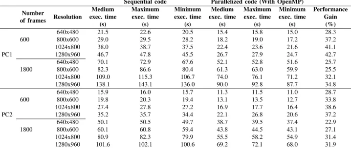
In order to study the influence of the dataset characteristics on the performance gains we tested the solution with another dataset from TUM,sequence 01, that was recorded at a higher resolution. The algorithm was tested varying the number of frames and the resolution of the dataset. The results are presented in table IV.

Every observation made for the last set of results can be observed once again on this table.

If we analyze the results for the increase of the image resolution we can conclude that we obtain increasingly better performance gains with higher resolutions. That is easily explained, higher image resolutions mean a larger amount of data per image and consequently more calculations to be made and, in that situation, more advantage is taken from parallelization. On the other hand, if we compare the results between 600 and 1800 frames we see that the performance gains are worse with a bigger dataset, i.e., more frames. This is also explained by the number of calculations. When the algorithm starts, all the information within the first frames is new, hence more keyframes are chosen and as a result there are more computation costs. Thus, as explained before, the algorithm takes more advantage of parallelization on the beginning of the dataset due to the larger amount of work on this phase.

Figure 1 demonstrates this same data in another perspective, which might be better to show the influence of these param-eters on the performance gain. The main observation that can be made is the fact that there is always a point where the performance gain starts to stabilize. That is more noticeable on the bottom figures, regarding performance gain vs number of frames, although, analyzing the other curves and their slopes we can expect that the same would happen. This behavior was expected, in every parallelization problem there is a point where the increase of the amount of work will not lead to better performance gains.

A. FPS Analysis

Frames per second, FPS, was a challenging parameter to study due to its unexpected results.

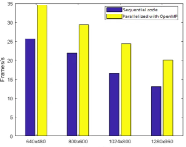
Figure 2, using the data from table IV, shows the gains on FPS obtained with our solution, which represents a good improvement. Nevertheless, from this figure, a first unexpected observation can be made. Comparing the FPS values, running on the same PC, between the two datasets, 600 and 1800 frames, we can observe a drop in FPS. For instance, on PC1, with 640x480 resolution, dataset with 600 frames runs with 38 FPS but dataset with 1800 frames presents only about 34 FPS. The difference is small, but exists and happens in every situation.

TABLE III: Execution times and performance gains for datasets using different number of frames.

Sequential code Parallelized code (with OpenMP) Dataset Medium exec. time (s) Maximum exec. time (s) Minimum exec. time (s) Medium exec. time (s) Maximum exec. time (s) Minimum exec. time (s) Performance Gain (%) freiburg1 xyz 39.4 40.4 37.7 32.0 33.9 30.1 18.8 freiburg2 xyz 85.8 96.1 83.2 61.5 64.1 58.7 28.3 PC1 freiburg3 sittting xyz 47.1 50.7 44.6 27.9 29.3 25.0 40.8 freiburg2 desk 108.2 116.6 104.8 81.2 83.6 78.1 24.9 freiburg3 teddy 123.0 138.2 118.3 96.1 101.7 86.2 21.8 freiburg1 xyz 27.3 27.8 26.8 20.6 21.5 19.9 24.5 freiburg2 xyz 60.2 60.4 59.9 43.0 43.8 42.5 28.6 PC2 freiburg3 sittting xyz 33.3 34.7 31.7 18.8 19.8 18.3 43.5 freiburg2 desk 76.1 77.1 74.8 55.6 56.2 55.1 27.0 freiburg3 teddy 85.6 89.4 84.2 62.2 67.7 55.4 27.4

TABLE IV: Execution times and performance gains for datasets using different number of frames and resolutions. Sequential code Parallelized code (With OpenMP)

Number of frames Resolution Medium exec. time (s) Maximum exec. time (s) Minimum exec. time (s) Medium exec. time (s) Maximum exec. time (s) Minimum exec. time (s) Performance Gain (%) 640x480 21.5 22.6 20.5 15.4 15.8 15.0 28.3 600 800x600 29.0 29.5 28.2 18.2 19.0 17.2 37.2 1024x800 38.0 38.7 37.5 22.4 23.6 21.6 41.1 PC1 1280x960 46.7 47.8 45.5 26.7 27.9 24.7 42.7 640x480 70.1 72.9 67.6 52.1 52.8 51.6 25.7 1800 800x600 82.3 86.6 80.4 61.3 63.0 59.9 25.5 1024x800 109.0 115.3 106.7 74.0 76.1 71.2 32.1 1280x960 138.1 143.1 136.0 90.0 92.8 87.7 34.8 640x480 15.9 16.0 15.7 11.3 11.5 11.0 28.7 600 800x600 19.8 20.3 19.4 13.1 13.5 12.7 33.8 1024x800 27.4 27.8 27.2 16.9 17.7 16.4 38.6 PC2 1280x960 35.2 35.7 34.4 22.1 26.8 20.6 37.2 640x480 50.1 50.5 49.7 38.7 39.5 37.4 22.9 1800 800x600 60.1 60.8 59.4 43.8 44.5 43.1 27.1 1024x800 80.9 82.3 79.9 55.5 58.2 54.9 31.4 1280x960 101.6 102.1 100.6 69.2 72.1 68.0 31.9

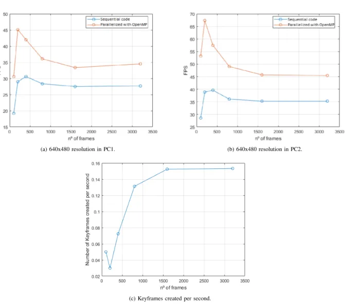
At first sight, the number of frames of a dataset should not affect the number of FPS. Thus, in order to verify this statement, figures 3a and 3b were constructed, in a similar way to figure 1 where we extended the tests for a larger number of frames. These figures show the FPS evolution when varying the number of frames of the dataset, for 640x480 resolution, on the two PCs. These figures show that the number of frames indeed affects the FPS parameter.

In order to interpret these results we need to make a more deep analysis and take in consideration the many steps and functioning of the algorithm. One aspect that is highly correlated with FPS is the number of keyframes created per second. The more keyframes chosen, the more calculations the algorithm has to perform. In fact, each keyframe selected causes the backend solver to run once again. In another note, the number of keyframes created depends strongly on the type of movements that the camera performs. If the movement is steady and slow, or if it stays focused on the same objects, few

or none new keyframes are created. On the other hand, if the movement is fast and moves to new places, a higher number of keyframes is chosen. Also, we have to consider that, in the beginning of a sequence, all the environment is new, so more keyframes are chosen to initialize the map.

With all the previous points taken into consideration, figure 3c represents the number of keyframes created per second for all the datasets with an increasingly number of frames. Since the number of keyframes created per second can be thought as the load of the algorithm, and its evolution curve, figure 3c, is approximately symmetrical with the FPS evolution we can, consequently, accept this as the plausible explanation for this unpredicted behavior. There are many characteristics of this curve that we can identify as a result of the points we explained earlier. For instance, we see that from 100 to 200 frames there is a drop on the number of keyframes created per second, which causes the increase in FPS. That is explained by the fact that, when the algorithm is initializing, it still has no

(a) Execution profile in PC1. _{(b) Execution profile in PC2.}

(c) Execution profile in PC1. (d) Execution profile in PC2.

Fig. 1: Performance gain (Y-axis) influenced by resolution (top row) and number of frames (bottom row).

information about the environment and therefore has to accept keyframes at a higher rate. Once the initialization is completed, after 100 frames, only frames with new information will be used has keyframes and thus, fewer are created per second. After this process, the camera accelerates its movement, ex-plaining the increase on the number of keyframes created per second.

An important note to make about this study is that the figures presented in this section regarding the FPS evolution, do not represent the reality of all cases, because as we have seen before, they depend on many different aspects regarding the particular dataset and functioning of the algorithm. B. RAM and Cache Influence

As stated previously, RAM and Cache are also important specifications that need to be considered. In this section we address more deeply their influence and more importantly,

verify if the solution presented is limited by any of these components.

RAM is an important component as it stores data that is currently being used and allows fast read and write operations regardless of their physical location on the memory. Although, throughout this work RAM memory size proved not to be a limitation. The reason for that is simple. Going back in table I, we can see RAM specifications for both PCs,8 GB for PC1 and32 GB for PC2, thus all datasets used in this paper fit into memory. To have a base of comparison, a90 s dataset recorded at 640 × 480 resolution occupies 1.5 GB. Thus, only with a much larger dataset and/or recorded at a higher resolution would lead to RAM being a limitation.

Cache, on the other hand, proved different. A first indication that cache had a sugnificant influence was the fact that, when executing the same dataset repeatedly, a higher execution time for the first execution was measured. Thus, in order to verify

(a) Dataset with 600 frames in PC1. (b) Dataset with 1800 frames in PC1.

(c) Dataset with 600 frames in PC2. (d) Dataset with 1800 frames in PC2.

Fig. 2: FPS performance’s comparison between sequential and parallelized code forsequence 01 dataset.

if cache was indeed the explanation for this behavior, we forcefully emptied it between executions. Figure 4 shows the results of this experiment, where cache was emptied between 4th_{and 5}th_{execution, and between 8}th _{and 9}th _execution.

We observe that indeed there is an increase in execution time when cache is emptied. Note that, the dataset will only be stored on cache after the first execution. Thus, before it, the cache is still empty and that is the reason why the first execution presents a higher execution time. Another observation is that the increase in execution time is much higher on PC2 than on PC1. That is explained by the different cache specifications of both PCs (see table I). Note that the difference in memory space is not that much between both PCs, although that small difference generates a big discrepancy on the execution time increase.

V. PERFORMANCECOMPARISON WITHSTATE-OF-THE-ART

PARALLELIZEDSLAM ALGORITHMS

Through the years little effort has been made to parallelize SLAM algorithms, although there have been proposed a few solutions to different algorithms. This section focuses on com-paring the performance of our approach with three solutions, namely Accelerated ORB SLAM [15], Particle Filter SLAM using CUDA [16] and ORB SLAM 2 Optimization [17]. It is important to keep in mind that our approach parallelizes only for the CPU cores, while the solutions we compare against to were parallelized for GPU computing (see table V). Both [15] and [17] optimized the ORB SLAM algorithm and both pointed out that the ORB feature extraction represents the most time-consuming stage and thus was the focus of GPU paral-lelization. On the other hand, [16] developed work optimizing a particle filter-based SLAM using CUDA. In order to better understand the work and results of these authors we briefly

(a) 640x480 resolution in PC1. (b) 640x480 resolution in PC2.

(c) Keyframes created per second.

Fig. 3: FPS evolution with distinct number of frames for the DSO using the ”sequence 01” dataset. Also shown the influence of the number of frames on the number of keyframes created per second.

overview particle filter-based methods. In these methods, the system is represented by a set of particles, where each particle contains two types of data, the hypothetical state of the robot and the value of its weight. The state of the robot represents its position, with x, y, z coordinates and a fourth parameter that indicates the orientation. The particle weights represent how important the particle is, and consequently dictate the approximate robot location. The authors concluded that the most time-consuming task, representing a high percentage of work, performs the weight calculation, since the larger the number of particles the system has, the more accurate it is, and thus in each iteration the system computes a substantial number of weights.

Table V presents the best performance gains obtained for the different solutions. Note that our parallelized DSO solution presents a best performance gain of 43.5%, obtained on a dataset with 1200 frames, despite the fact that in figure 1c)

TABLE V: Comparison of the best performance gains between different optimized algorithms.

Platform Best performance Gain (%)}

ORB SLAM [15] GPU 35.5 ORB SLAM 2 [17] Ordinary GPU 50.0 Jetson TX1 70.6 Particle Filter SLAM [16] GPU 91.0 DSO (Proposed solution) (1260 frames) CPU 43.5

the performance gains reach up to61%. This value was not considered since it was obtained in datasets with extremely small number of frames (100), with the sole purpose of studying the influence of the number of frames in performance. In practical applications, it is unrealistic to consider using the algorithm for such small datasets.

The solution in [16] presents the best results by a large margin. By comparing with the other two, our proposal presents a performance gain that is not far from [17] and even

Fig. 4: Cache influence on execution times for both platforms PC1 and PC2.

surpasses the performance of [15]. This represents an inter-esting achievement, considering that the currently proposed solution is optimized only for the multicore CPU.

VI. CONCLUSIONS ANDFUTUREWORK

This paper first intended to obtain a better understanding of SLAM techniques and secondly, to accelerate, through parallelization techniques, a specific chosen SLAM algorithm. The second task was achieved by using several tools and frameworks, such as a profiler and the OpenMP API.

The use of a profiler provided vital feedback for the opti-mization, opening the possibility to easily visualize where the algorithm’s bottlenecks resided by examining a hierarchical tree of function calls ordered by execution times.

Throughout the development of this optimization tool chain, important decisions were possible. The first relates with the choice of the Direct Sparse Odometry (DSO) SLAM algorithm for parallelization, for a number of reasons stated before.

A second decision, and a more difficult one, was whether to parallelize for CPUs or GPUs. One of the reasons for adopting the CPU regards the hierarchical structure of the code. It proved to be too much encapsulated, being the work divided across a high number of function calls. In order to parallelize the several kernels for GPU execution using CUDA, the workload would have to be extremely heavy, otherwise it does not compensate the communications’ overhead. Another reason for this decision relates with the fact that, on future work, the algorithm will be used in low-power devices that lack a GPU embedded.

The choice to use OpenMP was quite straightforward. It uses a pragma-oriented model that provides a simple, flexible and user-friendly interface to develop parallelized code for multicores.

The results presented in this paper show speedups reaching up to 43.5% on standard datasets and proved reasonable

when compared with another optimization works based on GPU execution having a substantial higher number of cores. Furthermore, efforts to study the influence and limitations of other components such as cache memory were also performed. Obviously, GPU optimization has higher potential since it provides specialized processing able to perform fast calcula-tions. Although the work here presented makes use of OpenMP to perform CPU optimizations, the code can be restructured targeting GPU optimizations as well. In order to facilitate the development, OpenACC, a directive-based programming model developed by NVIDIA, can be used to offload C/C++ or Fortran code to an accelerator device, such as the GPU.

ACKNOWLEDGMENTS

This work was partially supported by Instituto de Telecomunicac¸˜oes and Fundac¸˜ao para a Ciˆencia e a Tecnologia (FCT), under grant UID/EEA/50008/2013 and PTDC/EEI-HAC/30485/2017.

REFERENCES

[1] J. Engel and T. Sch¨ops and D. Cremers, LSD-SLAM: Large-Scale Direct Monocular SLAM, European Conference on Computer Vision (ECCV), 2014.

[2] R. Mur-Artal and J. M. M. Montiel and J. D. Tards, ORB-SLAM: A Versatile and Accurate Monocular SLAM System, IEEE Transactions on Robotics, 2015.

[3] J. Engel and V. Koltun and D. Cremers, Direct Sparse Odometry, IEEE Transactions on Pattern Analysis and Machine Intelligence, 2018. [4] G. Klein and D. Murray, Parallel Tracking and Mapping for Small

AR Workspaces, 2007 6th IEEE and ACM International Symposium on Mixed and Augmented Reality, 2007.

[5] C. Pereira and G.Falcao and L.A. Alexandre, https://github.com/caap95/DSO˙Optimization.

[6] T. Sch¨ops and J. Engel and D. Cremers, Semi-Dense Visual Odometry for AR on a Smartphone, International Symposium on Mixed and Augmented Reality, 2014

[7] Klein, Georg and Murray, David, Improving the Agility of Keyframe-Based SLAM, Computer Vision – ECCV 2008, 2008

[8] Eade, E. and Drummond, T., Edge landmarks in monocular slam, British Machine Vision Conf., 2006

[9] A. Akbarzadeh and J. M. Frahm and P. Mordohai and B. Clipp and C. Engels and D. Gallup and P. Merrell and M. Phelps and S. Sinha and B. Talton and L. Wang and Q. Yang and H. Stewenius and R. Yang and G. Welch and H. Towles and D. Nister and M. Pollefeys, Towards Urban 3D Reconstruction from Video, 2006

[10] G. Klein and D. Murray, Parallel Tracking and Mapping on a camera phone, 2009 8th IEEE International Symposium on Mixed and Aug-mented Reality, 2009

[11] M. Irani and P. Anandan, All About Direct Methods, 1999

[12] R. A. Newcombe and S. J. Lovegrove and A. J. Davison, DTAM: Dense tracking and mapping in real-time, 2011 International Conference on Computer Vision, 2011

[13] M. Pizzoli and C. Forster and D. Scaramuzza, REMODE: Probabilistic, monocular dense reconstruction in real time, 2014 IEEE International Conference on Robotics and Automation (ICRA), 2014

[14] St¨uhmer, Jan and Gumhold, Stefan and Cremers, Daniel”, edi-tor=”Goesele, Michael and Roth, Stefan and Kuijper, Arjan and Schiele, Bernt and Schindler, Konrad, Real-Time Dense Geometry from a Hand-held Camera, Pattern Recognition, 2010

[15] Bourque, D., CUDA Accelerated Visual SLAM For UAVs, Master Thesis, Workcester Polytechnic Institute, 2017.

[16] H. Zhang and F. Martin, CUDA accelerated robot localization and mapping, 2013 IEEE Conference on Technologies for Practical Robot Applications (TePRA), 2013.

[17] ORB Slam 2 GPU Optimization, https://yunchih.github.io/ ORB-SLAM2-GPU2016-final/, 2016.

[18] Li, Mingyang and Mourikis, Anastasios I., High-precision, Consistent EKF-based Visual-inertial Odometry, Int. J. Rob. Res., 2013.