Optimization of technical trading rules in forex market using genetic algorithm

(1)

OPTIMIZATION OF TECHNICAL TRADING RULES IN

FOREX MARKET USING GENETIC ALGORITHM

Pedro Franco Silva

Project submitted as partial requirement for the conferral of Master in Finance

Supervisor:

Prof. Pedro Leite Inácio, Prof. Auxiliar, ISCTE Business School, Departamento de Finanças

(2)

Resumo

A análise técnica, juntamente com a análise fundamental, é uma das metodologias mais conhecidas que os traders utilizam nos mercados financeiros, com o propósito de prever a direcção do preço das acções através da análise do seu historial de preços. Esta análise tem como objectivo obter ganhos acima da média do mercado.

Nesta tese, pretende-se desenvolver estratégias fiáveis, no mercado cambial, através do processo de algoritmo genético, que tem como objectivo a optimização dos parâmetros dos indicadores da análise técnica (Double Crossover, Bollinger Band, MACD, RSI, Stochastic, Parabolic SAR, ADX). Os resultados obtidos pelas estratégias optimizadas são comparados com a estratégia Buy and Hold. Para verificar a robustez dos resultados obtidos utiliza-se o teste t, que permite provar se os resultados são estatisticamente significativos.

A amostra inclui os preços diários desde Janeiro de 2005 até Dezembro de 2011, o que permite analisar as diferentes fases do mercado financeiro – Tendência de subida, tendência de descida e neutra. A amostra também inclui a crise financeira que começou no verão de 2007.

Este estudo rejeita a hipótese do mercado eficiente, pois os resultados obtidos pelas estratégias obtiveram maior retorno que a estratégia Buy and Hold em ambos os períodos: in-the-sample (95%) e out-of-sample (60%). Adicionalmente, é possível concluir que os parâmetros optimizados no período de treino não oferecem garantia que os resultados sejam consistentes no período de teste.

Palavras-Chaves: Technical Analysis, Genetic Algorithm, Efficient Market Hypothesis, Backtesting,

(3)

Abstract

Technical analysis, along with fundamental analysis, are the one of the better known approaches used by traders in financial markets to forecast the direction of security’s prices through the study of historical market prices in order to obtain abnormal returns.

This paper aims to present a methodology for developing robust automated technical trading systems using genetic algorithms to the tuning of technical indicators parameters (Double Crossover, Bollinger Band, MACD, RSI, Stochastic, Parabolic SAR, ADX) in the context of foreign exchange market. The results obtained from the optimized strategies are compared against a benchmark strategy – Buy and Hold – and to conclude, the accuracy of the results are verified through a t-Test, in order to prove whether the results obtained are statistically significant or not.

The time span, from 2005 to 2011, covered to test the technical strategies contains all financial market phases – Bullish trend, bearish trend, and sideways –including the financial crisis that began in the middle of 2007.

This study refutes the efficient market hypothesis, since the results obtained by technical strategies can outperform the Buy and Hold strategy in both periods: in-the-sample (95%) and out-of-sample (60%). Additionally, this study shows that the parameters optimized from the training period cannot be guaranteed to be consistent for testing period.

Key words: Technical Analysis, Genetic Algorithms, Efficient Market Hypothesis, Backtesting

(4)

Numbers are like people; torture them enough and they will tell you anything. – Anonymous (quoted by John Ehlers in Rocket Science for Traders)

Acknowledgments

I would like to thank my supervisor Prof. Pedro Leite Inácio for his guidance and support over the realization of this thesis. I am also thankful to my family and my friends for their support and encouragement.

(5)

List of Figures

Figure 1 – Daily prices in-the-Sample period from January 1, 2005 to December 31, 2009 .... 12

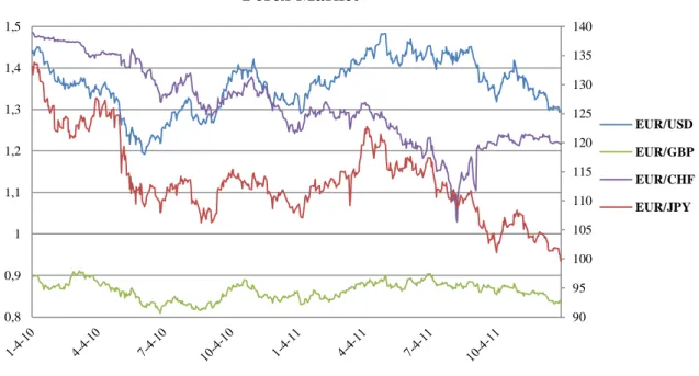
Figure 2 – Daily prices out-of-Sample period from January 1, 2010 to December 31, 2011 .... 13

Figure 3 – MetaTrader 4, Double Crossover indicator on EUR/JPY Daily price ... 22

Figure 4 - MetaTrader 4, Bollinger Band indicator on EUR/CHF Daily price ... 24

Figure 5 - MetaTrader 4, MACD indicator on EUR/GBP Daily price ... 26

Figure 6 - MetaTrader 4, RSI indicator on EUR/JPY Daily price ... 28

Figure 7 - MetaTrader 4, Stochastic indicator on EUR/USD Daily price ... 30

Figure 8 - MetaTrader 4, Parabolic SAR indicator on EUR/USD Daily price ... 32

Figure 9 - MetaTrader 4, ADX indicator on EUR/GBP Daily price ... 33

List of Figures

Table 1 - Parameters selected in Double Crossover trading strategy ... 9

Table 2 – General inputs for Technical Trading Systems... 16

Table 3 - Inputs selected in the Double Crossover Strategy ... 23

Table 4 - Inputs selected in the Bollinger Band Strategy ... 25

Table 5 - Inputs selected in the MACD Strategy ... 27

Table 6 - Inputs selected in the RSI Strategy ... 28

Table 7 - Inputs selected in the Stochastic Strategy ... 30

Table 8 - Inputs selected in the Parabolic SAR Strategy ... 32

Table 9 - Inputs selected in the ADX Strategy ... 34

Table 10 – Results obtained from the backtesting process for the seven technical trading strategies for both in-the-sample and out-of-sample period. ... 37

Table 11 - Annualized volatility ... 40

Table 12 – Final parameters optimized for the seven technical trading strategies through genetic algorithm process in-the-sample period ... 42

(7)

1 Introduction

Due due to the fast computational development, trading has become even more automated through the use of electronic trading platforms, which has allowed individuals to gain access to financial markets that could traditionally only be accessed by specialist trading firms, and as consequence it has increased the liquidity in the market. Hence, academic literature has been interested in the process of developing technical strategies through the process of evolutionary algorithm, where, firstly, it permits the parameters of the strategies being optimized more accurately by using extensive historical price data through the process of backtesting, and therefore the final selected strategies are used to execute automated trading orders in the market (algorithm trading), in order to achieve positive returns more constantly.

The aim of this study is to research trading in the foreign exchange market (Forex market) and to optimize the parameters of several automated trading strategies using a suitable programming language and to successfully test them with real market data. The purpose is to answer the following two questions:

 Is the market efficient or is it possible to achieve abnormal returns and beat the Buy and Hold (B&H) strategy?

 Is it possible to design a perfect technical trading strategy and use it successfully in the three phases of market – bullish, bearish and sideways?

This thesis is tested in four currency pairs – EUR/USD, EUR/JPY, EUR/GBP, EUR/CHF – and the data set includes the daily open and close prices from January 1, 2005 to December 31, 2011. The sample data is split in two periods: in-the-sample, which includes 5 years of historical data and where the parameters of technical strategies are optimized by genetic algorithm; and out-of-sample, which includes the remaining 2 years of data and where the optimized parameters are tested. During this period the financial markets has reached one of the most important financial crisis, subprime crisis, since Information Technology Bubble (dot-com bubble) in the beginning of the century. Consequently, this sample data is accurate because it includes all phases of market behavior – bullish, bearish and sideways market.

(8)

In the process of designing the technical strategy a special attention is given to the optimization of risk management parameter, which by itself can have an important influence in the final result obtained by the strategy.

The technical indicators tested in this paper are: Double Crossover, Bollinger Bands, RSI, MACD, Stochastic, Parabolic SAR, and ADX.

This paper is structured as follows: Section 2 describes parts of the existing literature regarding the methodology covered, namely the concepts of efficient market hypothesis theory, behavioral theory, random walk, technical analysis and fundamental analysis. Section 3 introduces the methodology of genetic algorithms. The data and methodology used are presented in section 4, while the technical trading rules are explained in section 5. Finally, in section 6 the results obtained are analyzed and discussed, with section 7 concluding and providing an outlook on future work.

(9)

2 Literature Review

In the past decades, academic literature has published different studies both empirically and theoretically regarding the consistency of the efficiency of financial markets. The oldest theory, Efficient Market Hypothesis (EMH), was developed in the mid-1960s by Alexander (1964), Fama and Blume (1966), which states that security prices reflect all the information that is available to investors, and as a consequence, one cannot consistently achieve returns in excess of average market returns on a risk-adjusted basis. Besides that it also supports the random-walk theory. More recently, the Behavioral finance theory has been researched by psychologists such as Kahneman and Tversky (1979), and Thaler (2005) in order to interpret the anomalies literature, which believes that there are several “irrationalities” behind individuals decisions on financial markets. These irrationalities can be considered a combination of cognitive bias, such as overconfidence, overreaction, behavioral biases, forecasting errors, and other types of human errors in reasoning and information processing. Thus, behavioral finance claims that the market is inefficiency through the effects of social, cognitive, and emotional factors on the economic decisions of individuals and as a consequence these factors deviate prices from their “correct value” and originate incorrect probability distributions about future rates of return. Further information about these two theories will be described later in this section.

The forecasting of security prices is one of the most challenging application areas in the financial market and it has received especial concern from the academic literature. Currently, forecasts are made through the use of either technical analysis or fundamental analysis. Moreover, the definition of both analyzes will be described.

Technical Analysis agrees with the behavioral finance theory. As defined by Kaufman (2005), technical analysis is the systematic evaluation of price, volume, breath and open interest, for the purpose of price forecasting. It may include any quantitative analysis as well as all forms of pattern recognition (charts).

Charles Dow, who founded The Wall Street Journal, is considered the grandfather of technical analysis due to the work he developed at the end of 19th century, by analyzing market behavior, which later became known as Dow theory. Through his research into market movements, he and his partner Edward Jones created the Dow Jones Industrial Average, in 1896.

(10)

Murphy (1999), summarizes the Dow theory in three main premises on which the technical analysis is based:

1. Market action discounts everything. 2. Prices move in trends.

3. History repeats itself.

1. Market action discounts everything: The technician believes that all relevant information that can possibly affect the price – fundamentally, politically, psychologically, or otherwise – is already reflected in the price of the market. As a consequence, the technician is not concern with the reasons why price rise or fall, instead he is only concern with the study of the market’s price.

2. Prices move in trends: The technicians believes that markets moves in trends, and its main propose is to identify those trends in early stages of their development in order to trade in its direction. The current trend is still moving in the same direction until it reverses, and then a new trend begins. The technician believes that through the quantitative analysis or by analyzing the patterns on the chart, they can predict when the trend is beginning to reverse.

3. History repeats itself: As said before, the technicians believe that the market prices are influenced by human psychology, which tends not to change, and then investors keep repeating their behaviors over and over again, which will originate recognizable and predictable price patterns on a chart. As an example, frequently, there are surveys about investors’ market sentiment, where they reveal whether they are bullish or bearish, which will make the market move in one or other direction, depending on the investor’ sentiment. On the other hand, the only way to forecast the future is by using the past price data and projecting those past experiences into that future, as a time series analysis.

Fundamental analysis consists on contrary principles of technical analysis, mainly its first premise, which states that market action discounts everything. Fundamentals focus on all the relevant factors that can influence the price of a market in order to determine the intrinsic value of that market. The intrinsic value is what fundamentals indicate as the real price of the security, based on the economic, industry and company analysis. Therefore, if the security’s price is below its intrinsic value, it is called undervalued, and the investor will buy the security, expecting the security to achieve its intrinsic value. Otherwise, it is called

(11)

overvalued and the investor will sell the security. The goal of both analyses is the same, which is to forecast the direction of the market. Fundamentals focus more on the medium/long term investment, while technicians concerns more on short-term investments. Besides that, both analyses can also be considered as an active management strategy, where the goal is to achieve abnormal returns – outperforming an investment benchmark index.

All these principles followed by technicians and fundamentals are rejected by efficient market hypothesis theory. As stated before, this theory was developed by Fama (1970) reviewed his initial study by dividing the EMH in three versions – weak-from, semistrong-form and strong-form.

The weak-form hypothesis affirms that security prices already reflect all information that can be derived from past price data, which is publicly available and virtually costless to obtain. This weak-form implies that technical analysis is worthless, because once a useful technical strategy is discovered, it would expected to be self-destructing when the mass of investors attempts to exploit it, and therefore, it will be automatically reflected in the price data. As a result, it is not possible for technicians to obtain abnormal returns. Furthermore, efficient market hypothesis defends that security prices changes in response to unpredictable new information, thus, price moves is unpredictable. This argument follows the Random Walk Theory that claims that prices changes are independent and identically distributed and that historical price is not reliable to predict the future, as stated by Malkiel (1973).

The semistrong-form hypothesis affirms that all publicly available information, such as past price data and fundamental data, is already reflected in the security price. Again, once investors have access to such information from publicly available information, one would expect to be reflected in security prices, and therefore no abnormal returns will be achieved. Consequently, the semistrong-form refutes the fundamentals.

The strong-form hypothesis defends that security prices reflect all information of the firm, even insider information that is only available for the company.

In conclusion, the efficient market hypothesis believes that a passive investment strategy is the best way to invest in the market, due to the fact that it is not possible to outperform the market. A passive strategy is usually characterized by a buy-and-hold strategy, which focus on the long-term investment and consists on simple buying and then holding the security.

(12)

Despite all the academic literature in favor of the efficiency in financial markets and random-walk theory, there is strong evidence against efficient market hypothesis. As claimed by behavioral finance, the market is inefficiency because of the “irrationalities” of individual decisions in financial markets. This inefficiency verified argues with the fact that movement of price data does not follow a normal distribution, instead it proves the existence of fat tails in price data, which will create price distribution opportunities that allow investors to profit from it and obtain abnormal returns, as stated by Leigh et al. (2005).

In the past decades, there have been presented theoretically and empirical studies arguing in favor of both theories. Studies that provide evidence in favor of technical analysis are Brock et al. (1992), Karjalainen (1994), Bessembinder and Chan (1995), Mills (1997), and Lo and MacKinlay (2001). Whereas Hudson et al. (1996) and Allen and Karjalainen (1999) find evidence that is consistent with the efficient market hypothesis. However, the majority of the literature ignores the framework of parameter optimization, which has been increased, in past few years, through the use of computational intelligence techniques that is used to analyze extensive historical price data, in order to improve the accuracy of forecasting. The previews papers produced regarding parameter optimization through genetic algorithm have been verified excess returns when compared to a simple buy-and-hold strategy, Bessembinder and Chan (1995). Others authors, such as Karjalainen (1994), Allen and Karjalainen (1999), and Fahlenbrach and Strobl (2002) have also tested the use of evolutionary algorithms to the parameter tuning of trading rules.

(13)

3 Genetic Algorithm Optimization

Genetic algorithms (GAs) belong to the larger class of evolutionary algorithm, which consist of search, adaption, and optimization techniques based on the principles of natural evolution. It was developed by Holland (1962, 1975). There are other evolutionary algorithms, such as evolution strategies sourced by Schwefel (1981), evolutionary programming by Fogel et al. (1966), genetic programming Koza (1992), and others.

This paper uses the genetic algorithm technique in order to optimize the parameters of trading rules. GAs include many structures as potential candidate solutions and work with a high level of global sampling of the search space, which increases the likelihood of achieving a global optimum solution. However, the global optimum solution is not certain, normally, GAs’ generates robust near-optimal solutions to a wide range of problems. Dempster and Jones (2001). In these competitive financial markets achieving a near-optimal solution is an enormous advantage for traders, as they require a quick and robust solution instead of undergoing the lengthy process to find the overall optimal solution. Especially as once the optimal solution has been founded it is unlikely to stay the best one with future development in the financial market.

A genetic algorithm starts with a population of genetic structures, called chromosomes or string, which are randomly distributed in the solution space, Kim and Shin (2007). The size of the population influences both the ultimate performance and the efficiency of a genetic algorithm. A small population provides an insufficient sample size, which reduces the likelihood of achieving an optimal solution. However, a small sample only requires moderate computational performance. On the other hand, a large population requires a higher computational demand, which is due to a higher number of chromosomes that need to be evaluated, combined and mutated. Despite that, it includes an extensive enough data sample that increases the probability of converging to an optimal solution.

Therefore, each chromosome, which represents a potential solution of the target problem, is evaluated by defining a fitness criterion, or objective function, which ranks the chromosomes from the best to the worst. Through selection, the chromosomes with a high fitness criterion will be preserved and create more offspring; subsequently it becomes a greater part of the population and will be largely propagated from generation to generation, by replacing the poorly performing chromosomes. There are different selection methods to

(14)

perform reproduction in the GA – to choose the individuals that will create offspring for the next generation. This paper used the “roulette wheel”, Goldberg (1989), which is a method equivalent to a fitness-proportionate selection method for populations big enough.

The next step in genetic algorithm process is called crossover. Crossover is the process of cutting random strategy chromosomes pairs at randomly chosen points and exchanging tails between heads to make a new pair (offspring). In the crossover, only the chromosomes that have passed the fitness criteria are chosen, in order to increase the likelihood of creating a better chromosome. Afterwards, the resulting strings are analyzed to verify the uniqueness relative to the current population, and if the string is found to be unique, it will be placed in the least percentage of the population. The percentage of crossover rate used influences the efficiency of genetic algorithm. If a large rate is used, then it would lose the combination that had the highest fitness, once there is no guarantee that any of the offspring will be better. On the other hand, if a low rate is chosen, the search may stagnate due to the lower exploration rate.

Finally, the mutation operator is applied to genetic algorithm. Mutation is the process of randomly changing appropriate genes in the chromosome, where its main objective is to maintain or restore diversity in the population. As in crossover process, the percentage of mutation used influences the efficiency of genetic algorithm. A low level of mutation serves to preserve chromosomes with high fitness since in this type of optimization the goal is to search for optimal solution, or near-optimal solution. However, it reduces the possibility of introducing a new and better chromosome. If too many are mutated then there is a strong chance of losing the best chromosomes.

Each pass through the propagation, crossover and mutation process, it is expected that an initial population of randomly generated chromosomes will improve as parents are replaced by better offspring. The final solution is founded when both: the average fitness of the entire population does not increase after a few generations are created, or there is no improvement over the chromosomes with the best fitness. In order to improve the genetic algorithm, it can be run a several times to see whether it arrives at the same solution starting with different random values of the population. In conclusion, to verify the accuracy of the genetic algorithm, it is first optimized in-the-sample period, and therefore, the best solution obtained is tested in the out-of-sample period.

(15)

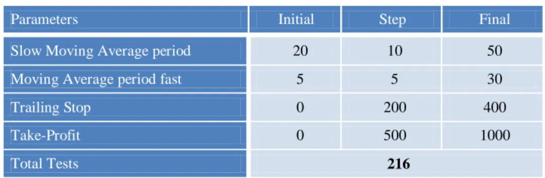
In order to better understand how this process of optimization by genetic algorithm is used in this paper, an example of the double crossover trading strategy is described:

Table 1 - Parameters selected in Double Crossover trading strategy

Parameters Initial Step Final

Slow Moving Average period 20 10 50

Moving Average period fast 5 5 30

Trailing Stop 0 200 400

Take-Profit 0 500 1000

Total Tests 216

Source: Author. This table includes the genetic population (pool) of the double crossover trading strategy.

The process of finding the best results of genetic algorithm is divided in the following six stages:

I. Initialization:

1. A chromosome (string) of 4 cells is created to represent each of the parameters. 2. Each cell (gene) in the string is assigned a random number that conforms to the predefined ranges.

II. Propagation:

3. The objective function (fitness criteria), which is explained in the section methodology, is calculated for each string.

4. The pool is ranked in descending order by fitness criteria.

5. Multiple copies are made of the highest-ranking chromosomes and added to the pool. III. Crossover:

6. Two strings, not previously selected, are chosen at random from the pool.

7. A random number between 1 and 4 divides the cells of the chromosomes into left and right parts.

8. The left part of the first string is switched with the left part of the second string, creating two new strings.

(16)

IV. Mutating:

10. One chromosome is chosen at random from the pool. 11. One of the 4 cells is chosen at random.

12. Based on the range of values for the parameter assigned to this cell, a new value is chosen at random.

13. Mutation continues until one cell in 10% of the chromosomes has been changed. V. Converging:

14. The best objective function, or fitness criteria, is saved at the end of each pass, and the parameter values associated with this chromosome are saved.

15. The genetic algorithm process continues at Step 3 until the objective function is achieved. That occurs when, after a number of passes, the objective function does not increase significantly.

16. The genetic algorithm process is repeated up to 5 times, beginning with the initialization.

17. After 5 passes, the chromosome previously saved with the highest objective function is the solution.

VI. Testing: (explained in the section Data)

18. The best objective function of genetic algorithm is optimized in-the-sample period. 19. The best objective function achieved in-the-sample, is then tested out-of-sample, in order to verify its accuracy.

(17)

4 Data and Methodology

In this section, the data and methodology used to calculate and optimize the rules of the indicators will be described.

4.1 Data

This paper was tested in the Forex market, which is the financial market for trading currencies. The foreign exchange market was chosen because it has specific characteristics that differ from the others financial markets. The foreign exchange market is the largest and most liquid financial market in the world, having an average daily turnover of $4.0 trillion (BIS, 12/2010)1 and it is open 24 hours a day except for weekends. The principal market participants are: non-reporting banks, central banks, corporations, governments, hedge funds, mutual funds, pension funds, brokers and others. It is traded in different financial instruments, such as spot transactions, forwards, swaps, futures, options markets and others. In this study, the use of spot market through electronic trading is the one that is used, which represents a good data sample because 40% of spot transactions are conducted on electronic trading systems due to advances in computing software and decrease of spread, with specially emphasizes in algorithmic trading (BIS, 12/2010).

The data set includes the bid and ask prices of the daily open and close prices (it also responds to market at one minute price for forced exits by the trailing stop and take-profit) of the foreign exchange market during the period from January 1, 2005 to December 31, 2011. These data was supplied by MetaQuotes Software Corp, which is the developer of the MetaTrader 4 online trading platform. This paper focus on the following currency pairs:

 EUR/USD – Exchange rate euro – American dollar

 EUR/JPY – Exchange rate euro – Japanese yen

 EUR/GBP – Exchange rate euro – British pound

 EUR/CHF – Exchange rate euro – Swiss franc

Despite all the currency pairs tested include the Euro, all of them have different characteristics that create singular market behaviors for each one, and therefore a good sample to be tested.

1

(18)

The amount of historical data covered and how to analyze it in order to develop the system is one of the most sensible steps in the process of designing a system, mainly due to the possibility of over fitting the data. Moreover, to analyze the accuracy of the system, the sample data was split in two periods – in-the-sample data (training period), as can be seen in Figure 1, and out-of-sample data (testing period), as can be seen in Figure 2.

There are some guidelines that can be taken into account to decide how to split the available data. For example, Azoff (1994) takes a typical approach, which suggests that the training period should be long enough to cover typical market behavior, including bull, bear and sideways moving markets. Kaufman (2005) suggests a 70:30 split between training and testing, while Kim and Lee (2004) suggests an 80:20 split.

Source: Author based on MetaQuotes

In conclusion, the main principle is to input as much diverse market behavior as possible with a long in-the-sample data, while keeping as long an out-of-sample data as possible to increase confidence to the model. Therefore, following those guidelines, this paper captures seven years of historical data, where five years will be used to optimize the technical indicator rules in-the-sample data (from January 1, 2005 to December 31, 2009), which represents 1298 trading days, and the remaining two years will be reserved for testing the best indicator (from January 1, 2010 to December 31, 2011), which includes 521 trading days. This originates a 60:40 split.

90 100 110 120 130 140 150 160 170 180 0,65 0,75 0,85 0,95 1,05 1,15 1,25 1,35 1,45 1,55 1,65 Forex Market EUR/USD EUR/GBP EUR/CHF EUR/JPY

(19)

During the in-the-sample period there are two strong trends: a bullish market until the middle of 2008 – despite financial crisis, subprime crisis, has begun in the summer of 2007, the bullish trend in foreign exchange market only reversed to a bearish trend in the summer of 2008 - and therefore a strong bearish trend took control of the market until the end of the in-the-sample period, end of 2009. Throughout the out-of-sample period the market has continued to decrease, however it has found some resistance levels where the market has been moving/moved sideways. In these sideways zones, the market volatility has increased comparing with the trend periods, which creates a good sample to test the best indicator optimized in the out-of-sample period, because it is tested in a different environment. It is important to reference that on September 6, 2011, the Suisse National Bank set a minimum exchange rate of 1.20 francs per euro, which has decreased its volatility since then.

4.2 Methodology

The aim of this study is to backtest several technical trading strategies in the foreign exchange market and to optimize its parameters through generic algorithm by using a suitable automated trading platform – MetaTrader 4 – and successfully test it with real market data – supplied by MetaQuotes. 90 95 100 105 110 115 120 125 130 135 140 0,8 0,9 1 1,1 1,2 1,3 1,4 1,5 Forex Market EUR/USD EUR/GBP EUR/CHF EUR/JPY

(20)

This section is divided in three parts: first, some trading concepts regarding foreign exchange market are explained. Therefore, the features applied to design the trading strategy are presented, and to conclude, it is described how to test the accuracy of trading strategies results against a benchmark strategy.

4.2.1 Trading Concepts

The standard contract size of currency pairs is one lot. Lot is a measure of the amount of base currency an investor is either buying or selling. One lot is worth 100000 units of base currency. It is possible to trade smaller lot sizes than 100000 units, such as mini lot (10000 units), micro lot (1000 units) and so on. As a consequence of trading this smaller lot sizes, the investor will add leverage to his trade, which means that the investor will trade with more money that he has. In foreign exchange market, leverage is normally indicated as a ratio, such as 100:1, in this case meaning that the investor can trade with 100 times the amount he has available for trading. As an example, if the investor buys a micro lot (1000 units), this means he just needs to invest an amount of 1000 units to trade the standard contract size (1 lot – 100000 units), therefore he is leveraging 100:1 times his trade.

Other important concept in trading is called pip (percentage in points), which is the smallest increment the quote of a currency pair can move. Different currency pairs might have different pip values, for example, the EUR/USD has a pip value of 0.00001 while the pip value of EUR/JPY is 0.001. The spread, slippage, trailing stop and take-profit are measured in pips, as can be seen in the Table 2.

4.2.2 Trading Strategy

As explained in the section Genetic Algorithm Optimization, all trading strategies are first optimized in-the-sample period through the process of genetic algorithm, and only the best parameters are then tested to the out-of-sample period. In order to evaluate each individual within the population, an evolution function and some restrictions are chosen, thus the algorithm can choose the best ones for reproduction, and then, converge on an optimal solution. The function chosen is the profit factor.

(21)

(1)

(2)

(3) Profit Factor function:

Other restrictions:

Where, if the profit factor function is higher than 1, the trading strategy has a positive return. If the profit factor is equal to zero, the final return is zero. If profit factor is lower than 1, then the strategy produces negative returns.

Therefore, the goal of the genetic algorithm is to maximize the profit factor function taking into account the restrictions applied to the trading strategies. The evolution terminates when there is no improvement in the selection period for a predetermined number of generations, or when a maximum number of generations are reached.

The profit factor strategy was chosen because it takes into account the profit made by the strategy; however, it also takes into consideration the risk produced by the strategy, where in this case the risk is measured by the total loss. Besides the total loss, the strategy rejects all the solutions produced by the genetic algorithm that has a percentage maximum drawdown higher than 25%, which is other measure of risk applied to the system.

%Maximal Drawdown function:

Where

In the case of the trading strategy has not achieved any positive result through the process of genetic algorithm optimization in-the-sample period, the best negative result is chosen and the restrictions are ignored, and therefore the best solution is tested out-of-sample period.

(22)

The trade entry (long or short) is always executed at the daily open price. However, the system responds to the market at the one minute price for forced exit by trailing stop or take-profit orders.

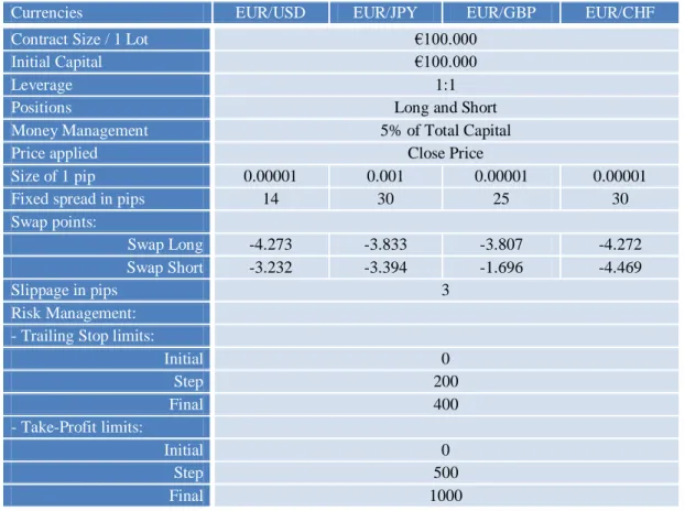
The general information applied to all trading strategies is presented in the following table:

Table 2 – General inputs for Technical Trading Systems

Currencies EUR/USD EUR/JPY EUR/GBP EUR/CHF

Contract Size / 1 Lot €100.000

Initial Capital €100.000

Leverage 1:1

Positions Long and Short

Money Management 5% of Total Capital

Price applied Close Price

Size of 1 pip 0.00001 0.001 0.00001 0.00001

Fixed spread in pips 14 30 25 30

Swap points:

Swap Long -4.273 -3.833 -3.807 -4.272 Swap Short -3.232 -3.394 -1.696 -4.469

Slippage in pips 3

Risk Management: - Trailing Stop limits:

Initial 0 Step 200 Final 400 - Take-Profit limits: Initial 0 Step 500 Final 1000 Source: Author

The specific inputs optimized in each trading strategy are exhibited on the section Technical Trading Rules.

The trading strategy is designed by taking into consideration three major features: rules to enter and exit trades; risk control; and money management, which follow the guidelines of Chande (1997).

 The rules to enter and exit trades will be discussed in detail in the next Section 5 Technical Trading Rules.

 Risk Management: In the context of financial markets, every investor has different types of risk tolerance, which can be divided in three categories – risk averse, risk neutral and

(23)

risk seeking – depending on how much risk one is willing to accept. Therefore, an investor places orders to sell (buy) securities to protect long positions (short positions) when losses cross predetermined thresholds. These orders are known as stop-loss. Thus, risk control might be defined as the process for managing open trades using predefined exit orders, where the stop-loss order is placed at the same time the trade is entered. If the price of the security falls, then a stop-loss is triggered and a loss is taken. How close stop-loss order will be placed to the actual price of the security, it depends on the investor risk appetite. A risk averse investor would place the stop-loss closer to the security price, which means that less money will be at risk if price falls, however the more likely it is that a smaller price fluctuation or random noise will hit the stop-loss. While a risk seeking investor would place the stop-loss further away from the security price, and consequently will have more money at risk but will be protected from the noise of the market. In order to manage the risk of open positions, there are other types of orders more complex than stop-loss, such as trailing stop orders. Trailing stop orders has the advantage of adjusting the threshold of a stop-loss if the price of the security rises. Therefore, a trailing stop will increase in value as the security price increase, always maintaining the same distance established initially, and it will never move down, thus once the price of the security falls, the stop will be triggered.

Besides the control of risk, the investor can also establish the amount of profit he is willing to achieve by placing a take-profit order. The use of stop-loss order and take-profit order originates the risk/reward ratio, which compares the expected return of an investment to the amount of risk undertaken to capture these returns. Normally, investors require a risk/reward ratio, at least, higher than 1 to execute the trade. As can be seen in Table 2, all the strategies are optimized by three levels of trailing stop and take-profit, where the values of take profit are always higher than the trailing stop, in order to achieve a risk/reward higher than 1. When the strategy includes these limit orders, positions are closed when the price hits their respective thresholds.

 Money Management: Consists on initial position size of the trade, taking into consideration the amount of capital of the portfolio and the potential trade risk. As every trade has the likelihood of carrying a possible loss, it is necessary to determine the maximum amount of capital to expose at each trade, which will be influenced by the investor’s risk tolerance. There are some approaches that can be used, such as calculating an optimal function to determine the exact amount to invest, defining a fixed amount of capital to invest,

(24)

or defining a fixed percentage of capital to invest in each trade. The fixed percentage of capital is the method chosen to apply on this study, because it adjusts the position size of each trade with the total amount of capital as the portfolio moves forward. The portfolio begins with a total capital of €100.000, and the position size of each trade is 5% of the total capital, which means that in the first trade only €5.000 are invested.

Besides these three major features that designed the trading system, there are other important aspects to look at when designing an accurate trading strategy. It is important to concern about the transaction costs applied to the system. Therefore, the results obtained will be compared against a benchmark (B&H strategy), and to conclude, the consistency of the results will be verified through a t-Test, to prove whether the results obtained are statistically significant or not.

4.2.3 Transaction Costs

This is one of the most important variables when designing a trading system, because by including transaction costs in the system, it can dramatically change the final result of the system from positive to negative results. The costs associated with forex trading has been changing in past few years, mainly due to the high liquidity in the foreign exchange market and to the increase of competition between brokers which helps to maintain the costs to a minimum. Despite that, brokers still execute some transactions costs to its clients when they trade in foreign exchange markets. The costs associated are: spread, slippage and rollover fees (swap points), which can be positive or negative.

 Spread: is the difference between bid and ask prices, where the bid price (the price at which the investor will sell) is always lower than the ask price (the price at which the investor will buy). This difference is the cost applied to each trade, which is measured in pips. The spread is never fixed, however brokers offered a possibility to trade with fixed spread, which was the case for this paper as can be seen in the Table 2. The spread also varies from one currency pair to another, mainly due to the difference in liquidity of each currency pair, where high liquidity means lower spread.

 Slippage: is the difference between the estimated transaction cost one expects and the actual transaction cost one gets. This means that, although a trade may be ordered at market open, this does not mean the trade will be opened (closed) at market open price. Slippage can happen due to the size of the order or because there are many orders scheduled, as there

(25)

(4) might not be enough liquidity to fill the entire order at the price the investor wanted. This strategy system accepted a maximum slippage of 3 pips, as can be seen in Table 2.

 Rollover fees: occurs when investors’ trades are holding overnight. Therefore, by maintaining its position open from one day to the other it has to be adjusted through the difference between the interest rates of the two currencies that form the currency pair. This difference between the interest rates are known as swap points rates, which are measured in pips as can be seen in Table 2. Moreover, if the investor buys into the currency with the higher interest rate, he will be paid the appropriate rollover amount at the start of the next trading session. Otherwise, the investor will be charged the correct rollover fees.

4.2.4 Benchmark

The results obtained in the training and testing period from the best trading systems will be compared with a benchmark strategy, the Buy and Hold strategy. As explained before, the Buy and Hold strategy consists on buying the market at the first day and keeping the position open until the end of the period analyzed.

The formula used to calculate the return of Buy and Hold strategy is:

Where

Therefore, when benchmarking a trading system, it is appropriate to perform a students t-test to determine the likelihood that the observed results is due to chance, as recommended by Kaufman (2005). The means of the strategies developed are tested against the null hypothesis of no excess returns, with a confidence level of 95%.

The hypothesis for the t-test would be: {

(26)

(5) The statistic of the test:

̅ √

Where ̅ is the sample mean, is the value under the null hypothesis, is the standard deviation of the sample and is the sample size.

The use of t-test consists on assumptions of normality and independence. Basically, these assumptions are limitations upon the utility of the t-test in evaluating trading systems. Normally, the assumption of normality is based on the Central Limit Theorem, which indicates that as the number of cases in the sample increases, the distribution of the sample mean becomes/converts normal. Therefore, as long as the sample size is acceptable (generally stated as at least 30), the statistic can be executed with accuracy.

In order to reject the null hypothesis with 95% confidence level, the p-value (marginal significance level ) should be lower than 0.05, and then the outcome is said to be “statistically significant”. Otherwise, the outcome is said to be “not statistically significant”. In conclusion, after benchmarking has been completed and tested its assurance, it gives the investor guidelines within which to operate. The investor can decide to trade using this strategy, and then it will be clear going forward whether the model is running within the expected guidelines. Besides that, it will give early warning if the model deviates from expectations by any change in markets behavior, giving the possibility for the investor to be able to manage it.

(27)

5 Technical Indicators Rules:

In this section the rules of the technical indicators used to calculate the best performance in the forex market are explained. Technical indicators are mathematical tools used to summarize all relevant information of the past history of a financial time series into short-term statistics. As stated before, the intend is to use different types of technical indicators - trend following systems (lagging indicators), momentum and oscillators systems (leading indicators) – in order to analyze different phases of market behavior from different perspectives.

 Trend following systems purpose is to identify trends in the market by smoothing the price data and removing markets noise. It does not lead the market, but rather follow the current direction with a lag. The simplest and most well known of all smoothing systems is the moving average. The lagging indicators work best when the market is trending, and is not effective in sideways markets, where it will likely lead to false signals (whipsaws).

 Momentum and oscillators systems purpose is to measure the rate-of-change of a security’s price. As indicators of change, they are used as leading indicators and can identify when the current trend is losing strength, that is, they demonstrate when an upwards move is decelerating, or vice versa, which permit to anticipate the market by giving early signals for entry or exit the market. These indicators are very useful in non-trending markets, where prices fluctuate in a horizontal price band, and they are also extremely valuable to identify when the market is overbought or oversold.

The indicators employed in this study are seven of the most popular technical indicators considered in academic studies and technical analysis literature (see, for example, Murphy (1999), and Kaufman (2005)): the Double Crossover method, RSI, MACD, Stochastic, Parabolic SAR, Bollinger Bands and the ADX. Note that there are more indicators that can also be used to attempt to gain more insight about market behavior, however, with the sample of indicators chosen, it is already possible to study the different market environments through the most important parameters.

(28)

(6)

5.1 Double Crossover Method

Double crossover method Murphy (1999) is characterized by using two distinct moving averages to generate market signals. One with a slower trendline, using a longer calculation period that has a longer lag, identifies the principal trend, which can be driven by government economic policy, such as modifying interest rates. The faster trendline is used for timing, which will give the signals to entry or exit the market in the direction of the principal trend. The final result may be more trades with smaller total profits, but a much more comfortable risk level for each trade. In this indicator two simple moving averages with different periods, which are determined through the optimization process, were used.

Simple moving average (arithmetic mean), averages the n past data prices P, maintaining the number of elements to be averaged the same, but the time interval, advances:

∑

(29)

For the Double Crossover method, as can be seen in the Figure 3, the rules to trade are:

 Buy when the close price of the faster moving average crosses (orange line) the slower moving average (blue line) going up, this is known as the golden cross;

 Sell when the close price of the faster moving average crosses the slower moving average going down, this is known as the dead cross.

 Positions are closed when the opposite of open order happens, i.e., the long position is closed when the close price of the slower moving average crosses the faster moving average going down.

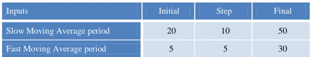
The specific parameters optimized in the double crossover strategy are described in Table 3:

Table 3 - Inputs selected in the Double Crossover Strategy

Inputs Initial Step Final

Slow Moving Average period 20 10 50

Fast Moving Average period 5 5 30

Source: Author

Comparing to the strategy of a simple moving average, it will give more signals and each time taking a small profit but with much smaller risk. Therefore, the false signals and whipsaws will decrease.

5.2 Bollinger Bands

This technique was developed by John Bollinger (2001). It is and indicator that allows users to compare volatility and relative prices levels over a period of time Murphy (1999). Two trading bands which are formed using the standard deviation (which changes as volatility increases or decreases) of the prices themselves and calculated over recent price history. The two bands are placed above and below a trend line, usually a moving average. Because the standard deviation represents a confidence level, depending on the number of standard deviation calculated, it ensures that 95,4% (in a 2 standard deviation example, and assuming that prices are normally distributed) of the price data will fall between the two trading bands, which will increase or decrease as volatility changes. As a rule, the prices are

(30)

(7) considered overbought when they touch the upper band, and oversold when they touch the lower band.

Standard deviation, is the most popular way of measuring the degree of dispersion of the data, which measure the average deviation from the mean.

√∑ ̅

Where ̅ is the average of all prices in the sample, n is the past data prices P.

The rules to trade the Bollinger Bands indicator are:

 Buy when close price comes below the lower band and then comes back into the trading bands.

 Sell when close price comes above the upper band and then comes back into the trading bands.

 Positions are closed when the close price cross the opposite band line.

(31)

(8) The specific parameters optimized in the Bollinger Bands strategy are described in the following table:

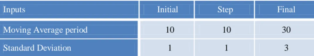
Table 4 - Inputs selected in the Bollinger Band Strategy

Moving Average period 10 10 30

Standard Deviation 1 1 3

Source: Author

5.3 Moving Average Convergence Divergence (MACD)

MACD was developed by Apple (1999). This indicator is one of the most reliable indicators available, Murphy (1999), because it turns two trend following indicators, exponential smoothed moving average (EMA), into a momentum oscillator by subtracting the difference between the two trends, which is called as MACD line. Therefore, this momentum value was further smoothed through a new exponential smoothed moving average of the MACD line, which originate the signal line. The difference between the signal line and the MACD line creates the MACD histogram that oscillates above and below a zero line, as can be seen in the Figure 5, which coincide with actual MACD crossover buy and sell signals. As a result, the MACD offers the best of both systems: trend following and momentum oscillator.

Exponential Smoothing Moving Average (EMA) is very similar to a simple moving average with the difference that it reduces the lag by applying more weight to recent prices.

Where

(32)

(9) (10) (11) MACD calculations: Where

There are different ways to trade with the MACD indicator. The most common use of the MACD is as a trend indicator. Therefore, the rules used are:

 Buy when both lines are below zero line and the MACD line (faster) crosses the Signal line (slower) from down-to-up.

 Sell when both lines are above zero line and the MACD line crosses the Signal line form up-to-down.

 Positions are closed when the opposite signal of open positions occurs, but it not contains the zero line condition.

(33)

(12)

(13) The specific parameters optimized in the MACD strategy are described in the following table:

Table 5 - Inputs selected in the MACD Strategy

Slow Exponential Smoothing Moving

Average period 20 6 32

Fast Exponential Smoothing Moving

Average period 9 3 18

Signal Line 6 3 12

Source: Author

5.4 Relative Strength Index (RSI)

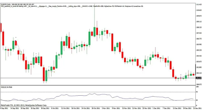
RSI was developed by Wilder (1978). It is an extremely popular momentum oscillator indicator that measures the speed and change of price movements. It provides added value to the momentum concept by scaling all values between 0 and 100. The RSI is especially used to identify when the market is overbought or oversold, expecting it to spend most of the time inside the specific boundaries, according to Wilder, 70 and 30. When the RSI moves higher or lower from those significant threshold levels, as we can see in the Figure 6, the market is read as overbought or oversold. At those levels, it generate buy and sell signals.

RSI calculations/formula: Where

(34)

The rules applied to trade the RSI indicator, as we can see in the Figure 6, are:

 Buy when the RSI indicator is below the oversold level (lower line) and crosses that line from down-to-up.

 Sell when the RSI indicator is above the overbought level (higher line) and crosses that line from up-to-down.

 Long/Buy position is closed when RSI indicator cross the higher line from down-to-up.

 Short/Sell position is closed when RSI indicator cross the lower line from up-to-down.

The specific parameters optimized in the RSI strategy are described in Table 6.

Table 6 - Inputs selected in the RSI strategy

Source: Author

RSI period 7 7 21

Higher Line 60 10 80

Lower Line 20 10 40

(35)

(16) (15) (14)

5.5 Stochastic

The stochastic indicator, created by George Lane, is an oscillator that measures the relative position of the closing price to the high-low range over a set number of periods. It is based on the commonly accepted observation that close prices tend do resist penetrating the previous resistance or support lines of the past few days. To calculate the stochastic indicator two lines are used – the %K line (main line), which is more sensitive, and the %D line (signal line), which give the signals to buy and sell – and it also uses the high, low and closing prices. There are two version of the stochastic indicator - the fast stochastic and the slow stochastic, which is a smoother version – and in order to produce them, three indicators are calculated, where the first two are used to produce the fast stochastic, and the last two are used to produce the slow version.

Stochastic formulas: ∑ ∑ Where

For the calculation of fast stochastic, the initial %K and %D fast formulas are used, while for the slow stochastic the %D fast and %D slow are used.

The formula simply measures, on a percentage basis of 0 to 100, where the closing price is in relation to the total price range for a selected time period, and as a bound oscillator, it identifies when the market is in overbought and oversold areas.

(36)

The rules used to trade the stochastic indicator are:

 Buy when the main line (%K, blue line) of the indicator is below the oversold level and main line crosses the signal line (%D, orange line) from down-to-up.

 Sell when the main line of the indicator is above the overbought level and main line crosses the signal line from up-to-down.

 Positions are closed when the opposite order should be opened.

The specific parameters optimized in the stochastic strategy are described in the follow table:

TABLE 7-INPUTS SELECTED IN THE STOCHASTIC STRATEGY

%K period 7 7 21 %D fast period 3 2 5 %D slow period 1 2 5 Higher Line 70 10 80 Lower Line 20 10 30 Source: Author

(37)

(20) (19) (18) (17)

5.6 Parabolic SAR

Developed by Welles Wilder, the Parabolic SAR is a price and time reversal system that is always in the market. It is a trend following indicator with an acceleration factor that decreases the lag between the indicator and the price as the trend extends over time. The indicator is below prices when prices are rising and above prices when prices are failing. In this regard, the indicator stops and reverses (SAR) when the price trend reverses and breaks above or below the indicator. To calculate the Parabolic SAR, Wilder used an acceleration factor, AF, with a defined initial value, which increases by the smoothing constant factor, SI, each time that a new extreme value occurs in the direction of the trend.

Parabolic SAR formulas:

Long positions, using the highest price:

Short positions, using the lowest price:

If there is a new extreme value in the direction of the trend, then:

Otherwise

(38)

The rules applied to trade the Parabolic SAR indicator are:

 Buy when the Parabolic SAR indicator crosses the price from up-to-down.

 Sell when the Parabolic SAR indicator crosses the price from down-to-up.

 Positions are closed when the opposite order should be opened.

The specific parameters optimized in the Parabolic SAR strategy are described in Table 8:

Table 8 - Inputs selected in the Parabolic SAR Strategy

SI – Smoothing constant factor 0.01 0.01 0.05 Maximum Acceleration Factor 0.1 0.1 0.3 Source: Author

5.7 Average Directional Index (ADX)

The ADX, minus directional indicator (-DI) and plus directional indicator (+DI) represent a group of directional movement indicators that form a trading system developed by Welles Wilder. The ADX measures trend strength without regard to trend direction, while +DI and –DI purpose is to define trend direction. The market is rising when +DI is higher than –DI, while the market is failing when +DI is lower than –DI. Used together, is it possible to determine both the strength and the direction of the trend. In order to analyze

(39)

whether the market is trending, the ADX indicator has to move above a threshold level that determines when the market is trending. If it crosses below that level, the market is consolidating.

The rules to trade the ADX indicator are:

 Buy when the ADX line (blue line) is above the threshold level (lower grey line) that determines when the market is trending and the +DI line (green line) crosses –DI line (red line) from down-to-up.

 Sell when the ADX line is above the threshold level that determines when the market is trending and the –DI line crosses +DI line from up-to-down.

 Positions are closed when ADX line went to level above higher line (higher grey line) and then crosses back under that level, or when +DI line and –DI line crosses.

(40)

The specific parameters optimized in the ADX strategy are described in the following table:

Table 9 - Inputs selected in the ADX Strategy

Source: Author

Open Level Line 20 5 30

Close Level Line 40 5 50

(41)

6 Empirical Results

In this section the results obtained through the backtesting process of each trading strategy are analyzed and interpreted. Where, firstly, a macro analysis is discussed by comparing the returns obtained from the technical trading strategies with a benchmark strategy – Buy and Hold strategy – and then analyzing the accuracy of the results. Secondly, a deeper analysis of the parameters optimized through the genetic algorithm process will be made, and also a comparison of both types of technical indicators: trending following and momentum oscillator indicator, to verify each one produced better results.

Overall, 96.4% of technical strategies optimized in the training period produced positive returns, which means that only one test had negative returns. When analyzing the optimized strategies out-of-sample period the profitability of the trading strategies reduced to 40%, however, during this period all the currency pairs were in a bearish market trend

Moreover, by comparing the results of technical systems against the Buy and Hold strategy can be concluded that both in-the-sample period (92%) and out-of-sample period (68%) the technical systems obtained higher returns than the B&H strategy.

To verify the accuracy of the results obtained through backtesting against the benchmark, the results of a student t-test are analyzed. Overall, only 20% of the tests were statistically significant with a 95% of confidence level. More precisely, in the optimization of the technical strategies period 30% of the tests were statistically significance, while in the testing period only 10% were verified to be statistically significant. This difference between both periods is mainly due to a smaller sample data used in the testing period, which originated less trades than in-the-sample period.

To finalize this macro analyze, where the results can be seen in the Table 102, it is possible to conclude that the technical strategies achieved better performance compared to B&H strategy in both periods, which proves the inefficiency of the forex market, and refuses the efficient market hypothesis. Despite that, it is also possible to conclude that even by optimizing the parameters of technical trading systems through a genetic algorithm process, these do not guarantee a profitable strategy in the future, where only 40% of the tests produced profitable returns in the testing period, mainly because financial markets are always

2

(42)

(21) changing, creating new patterns that will constantly produce inefficiencies in the trading strategies optimized in the training period.

Both the best range of technical indicators and individual technical indicator were evaluated through the formula of adjusted returns, Kaufman (2005):

Where it assumes that the actual trading performance is represented by the average of all tests, then adjusted it to a measure of risk, such as standard deviation.

Therefore, the momentum oscillator indicator (which includes: MACD, RSI and Stochastic) obtained higher adjusted returns for both in-the-sample and out-of-sample period than trend following indicator (which includes: Double Crossover, Bollinger Bands, Parabolic SAR and ADX), as can be seen in Table 10. From this analysis, it is also observed that by summing up all the results of each trading system both strategies obtained positive returns in-the-sample period, but negative returns in testing period.

The best individual indicator in-the-sample period is the Parabolic SAR with an adjusted return of 17%. Despite not being the indicator with higher average return, it is the indicator with lower volatility. In the testing period the RSI indicator achieved the higher adjusted return, which is a negative adjusted return of 6.5%. The only indicator that achieved positive average return out-of-sample period is the Bollinger Bands with 5.5% return, however it had an enormous volatility in its returns. These results can be seen in the Table 10.

(43)

TABLE 10–RESULTS OBTAINED FROM THE BACKTESTING PROCESS FOR THE SEVEN TECHNICAL TRADING STRATEGIES FOR BOTH IN-THE-SAMPLE AND OUT-OF-SAMPLE PERIOD.

These tables summarize the test results obtained in the training period (January 1, 2005 – December 31, 2009) and in the testing period (January 1, 2010 – December 31, 2012). In columns Stat. Sign. the values in bold are the ones that are statistically significant with a 95% confidence level. In the others columns, the bold values mean that the strategy optimized in the training period achieved results beyond the restrictions allowed in the design process of the system.

Double Crossover

In-the-Sample – From January 2005 until December 2009 Out-of-Sample – From January 2010 until December 2011

Total Profit Profit Factor #Trades %Profit Trades Max Drawdown B&H Stat. Sign Adjusted Return Total Profit Profit Factor #Trades %Profit Trades Max Drawdown B&H Stat. Sign Adjusted Return EUR/USD 68.562 3,76 41 95,12% 8,69% 5,67% 0,000 6,19% 10.669 1,58 18 88,89% 16,86% -9,56% 0,225 -23,6% EUR/JPY 108.072 2,89 41 56,10% 10,81% -4,11% 0,010 -4.710 0,83 16 43,75% 20,27% -25,17% 0,428 EUR/GBP 17.208 1,75 33 48,48% 9,27% 25,57% 0,090 -31.493 0,23 20 25% 33,31% -6,24% 0,007 EUR/CHF 12.545 1,8 39 56,41% 4,40% -4,03% 0,056 8.633 2,11 12 83,33% 6,92% -17,94% 0,157 Bollinger Bands

In-the-Sample – From January 2005 until December 2009 Out-of-Sample – From January 2010 until December 2011

Total Profit Profit Factor #Trades %Profit Trades Max Drawdown B&H Stat. Sign Adjusted Return Total Profit Profit Factor #Trades %Profit Trades Max Drawdown B&H Stat. Sign Adjusted Return EUR/USD 21.453 48,57 5 80,00% 1,16% 5,67% 0,079 -0,23% -7.679 0,46 4 25,00% 13,94% -9,56% 0,304 -42,34% EUR/JPY 5.699 1,07 73 82,19% 23,74% -4,11% 0,366 -56.589 0,27 27 74,07% 68,06% -25,17% 0,173 EUR/GBP 53.213 1,49 76 59,21% 12,66% 25,57% 0,043 44.779 2,67 30 73,33% 8,49% -6,24% 0,005 EUR/CHF 7.053 1,04 148 35,14% 29,04% -4,03% 0,358 41.680 1,27 46 34,78% 40,68% -17,94% 0,176