series
A. Manuela Gon¸calves
1, Marco Costa
2, Lara Teixeira
11 Departamento de Matem´atica e Aplica¸c˜oes, CMAT-Centro de Matem´atica,
Universidade do Minho, Portugal
2 Escola Superior de Tecnologia e Gest˜ao de ´Agueda, Universidade de Aveiro,
CMAF-UL, Portugal
E-mail for correspondence: [email protected]
Abstract: Change-points are present in many environmental time series. Time variations in environmental data are complex and they can hinder the identifi-cation of the so-called change-points when traditional models are applied to this type of problems. In this study, it is proposed an alternative approach for the ap-plication of the change-point analysis by taking into account this data structure (seasonality and autocorrelation) based on the Schwarz Information Criterion (SIC). The approach was applied to time series of surface water quality variables measured at eight monitoring sites.
Keywords: Change-point analysis; SIC; Autocorrelation; Seasonality; Mean and variance shift.
1
Introduction
In this study is proposed the application of the Schwarz Information Crite-rion (SIC) to detect the change-point in mean and variance in time series of water quality variables. The data concerns the River Ave hydrological basin situated in the Northwest of Portugal, where monitoring has be-come a priority in water quality planning and management in this wa-tershed. The water quality variable analyzed is Dissolved Oxygen (DO), one of the most important variables in assessing surface water quality in a river’s hydrological basin (Costa and Gon¸calves, 2011 and Gon¸calves and Costa, 2012), measured (in milligrams per liter (mg/l)) monthly from Jan-uary 1999 to December 2011 in eight monitoring sites: Cantel˜aes (CANT), Taipas (TAI), Ferro (FER), Gol˜aes (GOL), Vizela Santo Adri˜ao (VSA), Riba d’Ave (RAV), Santo Tirso (STI) and Ponte Trofa (PTR). In this work, the behavior study of the time series of DO water quality variable is ad-dressed in line with the research of Gon¸calves and Costa (2011), Gon¸calves and Alpuim (2011), who recently studied trend alterations in environmental variables, including time series of water quality variables. By performing an
exploratory analysis, we concluded that the DO observed values over time (each time series consists at most of 156 observations) presented changes in mean and/or variance in the series (in particular between 2004 and 2006). As regards the average, it apparently increases or decreases according to the monitoring site, but it reduces the variability of the observations in all monitoring sites, more evidently on some of them. Another important fea-ture is the indication of a seasonal component. This is due to the seasonal relationship between DO concentration with the weather patterns through-out the year, particulary temperature changes and precipitation intensity.
2
The informational approach
In order to detect changes in time series, the case of a change-point in both the mean and the variance, the aim is to test the following hypothesis
H0: µ1= µ2= . . . = µn = µ ∧ σ12= σ22= . . . = σn2 = σ2 (1)
versus the alternative hypothesis
H1: µI = . . . = µ1= µk �= µk+1= . . . = µn = µII
∧ (2)
σ2
I = σ21= . . . = σ2k�= σ2k+1= . . . = σ2n= σ2II.
Based on Akaike’s work, in 1978 Schwarz proposed the Schwarz Information Criterion (SIC). The SIC is defined as following
SICj =−2 ln L( ˆΘj) + pjln n, j = 1, 2, . . . , M, (3)
where n is the sample size. This criterion is based on the maximum like-lihood function of a given model penalized by the number of parameters that are estimated in the model. Under H0, the SIC is denoted by SIC(n)
and it is obtained as SIC(n) =−2 ln L0(ˆµ, ˆσ2) + 2 ln n, (4) = n ln 2π + n ln n � i=1 (Xi− X)2+ n + (2− n) ln n. (5)
where L0(ˆµ, ˆσ2) is the maximum likelihood function with respect to H0.
Under H1, the SIC is denoted by SIC(k) for fixed k, 2 ≤ k ≤ n − 2, is
obtained as
SIC(k) =−2 ln L1(ˆµI, ˆµII, ˆσI2, ˆσ2II) + 4 ln n (6)
where L1(ˆµI, ˆµII, ˆσI2, ˆσII2 ) is the maximum likelihood function under H1.
The decision to accept H0 or H1 is based on the principle of minimum
criterion. According to the information criterion principle, we are going to estimate the position of the change-point k such that SIC(k) is the minimal. Then, the estimation of the position of the change-point by ˆk is given by SIC(ˆk) = min
2≤k≤n−2SIC(k). In order to assess significance, a critical value
cα can be included in the decision rule for a significance level α, where
cα≥ 0. The model with a change-point SIC(k) is selected if
min
2≤k≤n−2SIC(k) + cα< SIC(n) (8)
otherwise, the model with no change-point SIC(n) is more reasonable. The approximate critical values for different series lengths that were obtained through the asymptotic distribution are presented in Chen and Gupta (1999).
3
Change-point detection procedure
The DO time series present statistical properties as a constant mean and seasonality whose parameters must be estimated at the same time. Thus, the adjusted model is
Xt(M 1)= µ + st+ �t, t = 1, . . . , n, (9)
where µ is the global series mean, st is the seasonal component and �t is
a white noise with E(�2
t) = σ2. The change-points detection considers the
errors series ˆ�t= Xt(M 1)− ˆµ − ˆst, t = 1, . . . , n.
The aim is to detect change-points in both the mean and the variance, i.e., to test the null hypothesis (1) versus the alternative hypothesis (2), through SIC application to the new series { ˆ�t}t=1,...,n, corresponding the
SIC(n) to the model (5) and the SIC(k) to the model (7). For a better understanding of the differences between information criterion values of the different models, will be represented SIC(k) values and the SIC(n)− cα
values for two significance levels, α = 0, 05 and α = 0, 01. If, statistically, a change-point is detected, a second model will be adjusted to the original data,
Xt(M 2)= µt+ st+ �t, t = 1, . . . , n, (10)
where stis the seasonal component for t = 1, . . . , n,,
µt= � µI if t≤ k µII if t > k and �t= � N (0, σ2 I) if t≤ k N (0, σ2 II) if t > k . After the adjustment of the model (10), it follows the binary segmenta-tion process with the second change-points detecsegmenta-tion, in the two errors
sequences, before and after change-point. However, the data analysis was conservative by taking into account the performed simulation study (not presented in this article) and in agreement with Beaulieu et al. (2012): the presence of autocorrelation in the observations, even weak ones (φ≈ 0.3), tends to originate the detection of false change-points. Thus, in this study when SIC(n) and SIC(k) values are very close, even if the change-point is statistically significant, we decided not to consider the existence of a second change-point.
4
Results and discussion
Taking into account the previous studies about this hydrological basin (Gon¸calves and Alpuim 2011, Costa and Gon¸calves 2011, Gon¸calves and Costa 2011) and the inspection of data series, it is reasonable to consider that the series do not present trends (for instance, a linear trend). More-over, works that compare DO data series (and other water quality variables, Gon¸calves and Alpuim 2011) in different water monitoring sites concluded that there is a common pattern in the evolution of these variables consid-ering the same hydrological basin. Thus, it is reasonable to consider the same change-point model for all eight water monitoring sites. The linear model M1 (9) was adjusted to DO data series (original data, without any transformation).
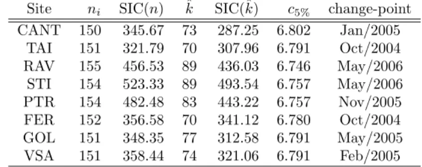
TABLE 1. Results of change-point procedures (ni-number of observations in site
i, ˆk = argmin2≤k≤154SIC(k)).
Site ni SIC(n) ˆk SIC(ˆk) c5% change-point
CANT 150 345.67 73 287.25 6.802 Jan/2005 TAI 151 321.79 70 307.96 6.791 Oct/2004 RAV 155 456.53 89 436.03 6.746 May/2006 STI 154 523.33 89 493.54 6.757 May/2006 PTR 154 482.48 83 443.22 6.757 Nov/2005 FER 152 356.58 70 341.12 6.780 Oct/2004 GOL 151 348.35 77 312.58 6.791 May/2005 VSA 151 358.44 74 321.06 6.791 Feb/2005
The SIC procedure was applied to all series according to the methodology shown above, considering the asymptotic critical values at a 5% significance level. Table 1 summarizes the results of SIC procedures. For all series was detected a change-point significant considering the respective critical value. One should notice that in all series the differences SIC(n)− SIC(ˆk) are clearly superior to the approximate critical values at a 5% significance level. Moreover, considering a 1% significance level, only the difference SIC(n)−
FIGURE 1. SIC(k) values for Cantel˜aes series and adjustment of linear model considering the change-point in Cantel˜aes.
SIC(ˆk) relatively to the Taipas series (TAI) is lower than the approximate critical value of c1% (for instance, c1% ≈ 15.079 when n = 150). Thus,
change-point procedures are assertive about the existence of a change-point in both mean and variance in each series, even considering a conservative significance level. For instance, Figure 1 represents SIC(k) values, 2≤ k ≤ 154, for Cantel˜aes series and the values SIC(n)− cαwith α = 1%, 5%.
As the assumptions of normality and independence are not present in some time series, a simulation study was carried out (not presented in this paper) in order to evaluate the methodology’s performance when applied to non-normal data series with or without time correlation.
References
Beaulieu, C., Chen, J., and Sarmiento, J.L. (2012). Change-point analysis as a tool to detect abrupt climate variations. Phil. Trans. R. Soc. A., 370, 1228 – 1249.
Costa, M. and Gon¸calves, A.M. (2011). Clustering and forecasting of dis-solved oxygen concentration on a river basin. SERRA, 25, 151 – 163. Gon¸calves, A.M. and Alpuim, T. (2011). Water quality monitoring using
cluster analysis and linear models. Environmetrics, 22, 933 – 945. Gon¸calves, A.M. and Costa, M. (2012). Predicting seasonal and
hydrome-teorological impact in environmental variables modelling via Kalman filtering. SERRA, (doi: 10.1007/s00477-012-0640-7).
Chen, J. and Gupta, A.K. (1999). Change point analysis of a Gaussian model. Statistical Papers, 40, 323 – 333.