F
ACULDADE DEE
NGENHARIA DAU
NIVERSIDADE DOP
ORTOEnergy-aware resource management for
heterogeneous systems
Eduardo Fernandes
Mestrado Integrado em Engenharia Informática e Computação Supervisor: Jorge Barbosa
Energy-aware resource management for heterogeneous
systems
Eduardo Fernandes
Mestrado Integrado em Engenharia Informática e Computação
Abstract
Nowadays computers, be they personal or a node contained in a multi machine environment, can contain different kinds of processing units. A common example is the personal computer that nowadays always includes a CPU and a GPU, both capable of executing code, sometimes even in the same integrated circuit package. These are the so called heterogeneous systems.
It’s important to be aware that the various processing units aren’t equal, for instance CPUs are very different from GPUs. This raises a problem, since not every task can be executed in all processing units.
To solve this problem a new task scheduling algorithm was developed with the aid of SimDag from the SimGrid toolkit. This algorithm uses a DAG (directed acyclic graph) to aid the scheduling of different tasks, be they from a single application or from various different applications.
The algorithm is based on the HEFT scheduling algorithm, a greedy algorithm with a short execution time, developed by Topcuoglu et al. This new algorithm is aware of the different pro-cessing units and of the different performance/power levels. This solves the problem of not all tasks being able to be executed in all processing units.
Since previous studies show that reducing the CPU clock speed on DVFS (dynamic voltage frequency scaling) CPUs can reduce the energy spent by the CPU while executing various tasks with little increase in runtime. Various tests were made to obtain the power rating of a test CPU while operating on different performance levels. With this it was possible to obtain performance and power information on the power states, this information is then later used by the algorithm in order to find the optimal performance/power ratio.
The algorithm main objective is to spend the least amount of energy possible, in contrast to the HEFT goal that is to execute tasks as fast as possible. The algorithm behavior can be modified by changing the minimum power state that the processing units should run or by changing the goal. Two goals are provided, the EFT (earliest finish time) from the original HEFT algorithm and the LEC (least energy cost). Both goals are affected by the defined minimum power state.
Using this new algorithm it was possible to reduce total energy spent some times at the cost of increased runtime.
Resumo
Nos dias de hoje os computadores quer sejam pessoais ou um nó contido num ambiente multi maquina, podem conter diversos tipos de unidades de processamento. Um exemplo comum é o computador pessoal que nos dias de hoje inclui sempre um CPU e um GPU ambos capaz de executar código, muitas vezes no mesmo circuito integrado. Estes sistemas são heterogéneos.
É importante estar consciente que as varias unidades de processamento não são iguais. Por exemplo os CPUs são bastante diferentes dos GPUs. Com isto surge um problema, pois nem todas as tarefas podem ser executadas em todas as unidades de processamento.
Para solucionar este problema um novo algoritmo de escalonamento foi desenvolvido recor-rendo ao SimDag pertencente ao toolkit do SimGrid. Este algoritmo utiliza um DAG (grafo dire-cionado acíclico) para facilitar o escalonamento de diferentes tarefas, sejam elas provenientes de uma única aplicação ou de várias aplicações diferentes.
Este algoritmo é baseado no algoritmo de escalonamento HEFT desenvolvido por Topcuoglu et al. É um algoritmo ganancioso, mas de rápida execução. Este novo algoritmo está ciente tanto das varias unidades de processamento como dos diferentes níveis de performance/potência. Com isto o problema de nem todas as tarefas poderem executar em todas as unidades de processamento fica resolvido.
Visto que estudos anteriores mostram que reduzindo a frequência de relógio do CPU em sis-temas baseados em DVFS (sissis-temas de escalamento dinâmico de voltagem e frequência) os CPUs podem reduzir a energia gasta a executar diferentes tarefas com um pequeno aumento no tempo de execução. Vários testes foram efetuados para obter a potência consumida por um CPU en-quanto este operava em diferentes níveis de performance. Com isto foi possível obter informação a cerca da performance e respetiva potência relativos aos diversos níveis de performance, esta informação é depois utilizada pelo algoritmo de maneira a encontrar o rácio mais vantajoso de performance/potência.
O objetivo principal do algoritmo é gastar a menor quantidade de energia possível, isto em contraste com o HEFT cujo objetivo é executar as tarefas o mais rápido possível. O comporta-mento do algoritmo pode ser modificado alterando o estado de energia mínimo que as unidades de processamento devem executar ou alterando o objetivo. Dois objetivos são fornecidos, o EFT (tempo para completar mínimo) do algoritmo original HEFT e o LEC (menor custo de energia). Ambos os objetivos são afetados pelo estado de energia mínimo definido.
Utilizando este novo algoritmo foi possível reduzir o total de energia gasta. As vezes a custa do aumento do tempo de execução.
Acknowledgements
I would first like to thank my supervisor Jorge Barbosa for all the input and advice given during the development of this thesis. I would also like to thank to all the people from the SPeCS research group at FEUP for the input given.
I would like to thank my family and friends for helping and supporting me at all times. I am very grateful by the constant help and support from Vanessa Ramos.
I would like to thank Ricardo Coutinho for the help given reviewing this thesis.
“Don’t kick the robots.”
Contents
1 Introduction 1
1.1 Problem statement . . . 1
1.2 Motivation and Objectives . . . 1
1.3 Dissertation Structure . . . 2
2 Background 3 2.1 Introduction . . . 3
2.2 Computing System Types . . . 3
2.2.1 Homogeneous Systems . . . 3
2.2.2 Heterogeneous Systems . . . 3
2.3 Task Graphs . . . 5
2.3.1 Directed Acyclic Graph (DAG) . . . 6
2.4 Scheduling Algorithms . . . 7
2.4.1 Best-effort . . . 7
2.4.2 QoS-constraint . . . 7
2.5 Power Consumption Measurements . . . 8
2.5.1 Internal Hardware Counters . . . 8
2.5.2 External Hardware . . . 8
2.6 Available Simulation Tools . . . 10
2.6.1 Comparison between tools . . . 11
2.7 Available Energy Consumption Reporting Tools and APIs . . . 12
2.7.1 Comparison between tools . . . 13
3 Methodology 15 3.1 Introduction . . . 15
3.2 Power and Energy Analysis . . . 15
3.2.1 CPU . . . 16
3.2.2 GPU . . . 17
3.2.3 GPU speed control . . . 18
3.3 Performance Analysis . . . 19
3.3.1 Chosen Benchmarks . . . 19
3.3.2 Outputs . . . 20
3.4 Simulated Platform Model . . . 21
3.4.1 SimGrid Platform Model . . . 21
3.4.2 SimGrid Platform Model limitations . . . 21
3.5 Task Graph Model . . . 23
3.5.1 SimGrid Task Model . . . 23
CONTENTS
3.5.3 SimGrid Task Graph Model limitations . . . 24
3.5.4 Contech . . . 25 4 Scheduler 27 4.1 Proposed Algorithm . . . 27 4.1.1 Introduction . . . 27 4.1.2 HEFT Algorithm . . . 27 4.1.3 HLEC Algorithm . . . 28 4.2 Implementation . . . 29 4.2.1 Program structure . . . 29 4.3 Input Files . . . 30 4.3.1 Configuration Files . . . 30 4.3.2 Graph . . . 31 4.3.3 Platform . . . 32
4.4 SimGrid library modification . . . 34
4.4.1 Host speed change in runtime . . . 34
4.5 Conclusions . . . 34 5 Results 35 5.1 Task Graph . . . 35 5.1.1 Contech . . . 35 5.1.2 Existing examples . . . 35 5.1.3 Manually created . . . 35 5.1.4 Simulation Results . . . 36
5.1.5 Comparison between HEFT and HLEC algorithms . . . 38
5.2 Hardware Performance and Energy Results . . . 40
5.2.1 CPU only, Intel Core i7-4500U . . . 40
5.2.2 Test Platform Model . . . 46
6 Conclusions and Further Work 47 6.1 Attained Goals . . . 47
6.2 Study limitations and further work . . . 47
6.2.1 Limitations . . . 47
6.2.2 Further Work . . . 48
References 49 A SimGrid Platform Files 51 A.1 XML File . . . 51
A.2 JSON File . . . 51
B Benchmark results 55 B.1 Performance - Linpack . . . 55
B.2 Energy - Linpack . . . 62
C SimGrid modifications 65 C.1 Runtime host speed change . . . 65
List of Figures
2.1 Simple Graph . . . 5
2.2 Sample Task Graph . . . 5
5.1 Sequential Test HLEC scheduler result . . . 36
5.2 Parallel Test HLEC scheduler result . . . 36
5.3 Montage 100 HEFT scheduler result . . . 37
5.4 Montage 100 HLEC scheduler result . . . 37
5.5 SimGrid Runtime vs Energy results . . . 39
5.6 Linpack Power vs Energy benchmark results (big configuration) . . . 41
5.7 Linpack Execution time vs Energy benchmark results (big configuration) . . . 42
5.8 Linpack Execution time vs Energy benchmark results (mixed configuration) . . . 44
LIST OF FIGURES
List of Tables
2.1 Comparison between simulation tools . . . 11
3.1 Values provided on by the Intel Power Gadget on an i7-4500U . . . 16
3.2 Modified Intel Power Gadget sample output on an i7-4500U CPU . . . 17
3.3 DAX job tag attributes . . . 24
3.4 DAX file tag attributes . . . 25
4.1 JSON job attributes . . . 32
4.2 JSON host attributes . . . 32
5.1 Scheduler time and energy outputs . . . 38
5.2 PState settings on an i7-4500U CPU (Linpack, 2 cores active) . . . 40
5.3 Time and energy differences between frequencies, i7-4500U CPU . . . 46
B.1 Linpack Benchmark - Big Configuration Performance Results . . . 56
B.2 Linpack Benchmark - Small Configuration Performance Results . . . 57
B.3 Linpack Benchmark - Mixed Configuration Performance Results (1/4) . . . 58
B.4 Linpack Benchmark - Mixed Configuration Performance Results (2/4) . . . 59
B.5 Linpack Benchmark - Mixed Configuration Performance Results (3/4) . . . 60
B.6 Linpack Benchmark - Mixed Configuration Performance Results (4/4) . . . 61
B.7 Linpack Benchmark - Big Configuration Energy Results . . . 62
B.8 Linpack Benchmark - Small Configuration Energy Results . . . 62
LIST OF TABLES
Abbreviations
API Application Programming Interface CPU Central Processing Unit
CUDA Compute Unified Device Architecture DAG Directed Acyclic Graph
DRAM Dynamic Random-Access Memory DSP Digital Signal Processor
DVFS Dynamic Voltage and Frequency Scaling FLOPS Floating-Point Operations Per Second FPGA Field Programmable Gate Array
GLOPS Giga Floating-Point Operations Per Second
GPGPU General Purpose computing on Graphic Processing Units GPU Graphics Processing Unit
HPC High Performance Computing IC Integrated Circuit
MSR Model Specific Registers NVML NVIDIA Management Library RAM Random-Access Memory RAPL Running Average Power Limit SoC System-On-Chip
TFLOPS Tera Floating-Point Operations Per Second TDP Thermal Design Power
TSC Time Stamp Counter ULV Ultra Low Voltage WWW World Wide Web
Chapter 1
Introduction
1.1
Problem statement
Nowadays different kinds of processing units exist (CPUs, GPUs, special purpose accelerators, among others) and some times more than one processing unit is present in a single computing system.
Many examples of this exist: a typical laptop computer usually includes two different pro-cessing units (CPU and GPU), the highly integrated SoC present on a smart phone also includes various processing units (CPU, GPU, DSP, some times others), to high performance computing grids that use large amounts of processing units. All these systems are heterogeneous, since they employ different processing units with distinct characteristics and most of the times with different architectures.
These systems pose a new problem: leveraging the right architecture for the task at hand. This leads to increasing research efforts on how to leverage computing power from these systems.
High Performance Computing is an important area that many fields depend upon. Heavy computing reliant domains like climate research, molecular modeling, weather forecasting, aero-dynamic modeling and others can benefit from higher throughput and better energy efficiency.
Since many of these computations need to be finished in useful time or within some financial cost, most of the times models have their accuracy reduced to finish computation faster and stay within budget. This problem can be solved by providing more efficient computing power so that more accurate models can be used.
1.2
Motivation and Objectives
Currently there is a demand for high computing power, but it comes at a very high cost, be it financial, temporal or energetic.
Many times the software doesn’t take advantage of the existing hardware. One example is the rise of multi-core CPU and the lack of proper use of the multiple cores present in the system. Another example is the lack of use of GPUs for computational purposes.
Introduction
With this comes the need or better leveraging of different processing units present in computer systems.
Since there are various computing architectures available, with different characteristics, many times in the same machine there is the need to better use those architectures. Different architectures have distinct advantages and disadvantages, so leveraging the correct architecture for a specific task might provide lower costs and increase performance.
The main objective is to create a scheduling algorithm that optimizes the use of current hetero-geneous computing platforms and better distribute tasks while being aware on the energy spent.
This work is being developed under the Antarex project, whose objective is to provide a way to manage and auto tune applications in order to reach exascale computing at around 20 Megawatts. In order to reach this goal the Antarex project proposes controlling all the decision layers, in order to implement a self-adaptive application optimized for energy efficiency [SL].
1.3
Dissertation Structure
This dissertation is divided in six chapters, the first is a brief introduction (this chapter). It is followed by the second chapter where the literature review and related work are presented. The third chapter explains the used methodology. The fourth chapter contains the obtained results. The fifth chapter contains the implementation details. Finally the last chapter is where the conclusions and further work are discussed.
Chapter 2
Background
2.1
Introduction
In this chapter the literature review and related work are presented. Different computing system types are also explored. A small introduction to task graphs and scheduling algorithms is given. The main tools usable in this project will also be discussed.
2.2
Computing System Types
In this section different computing system types will be discussed: homogeneous and heteroge-neous systems.
2.2.1 Homogeneous Systems
An homogeneous computing system is a system that uses only one kind of processor. One example is a headless computer that only has a kind of processing unit like a CPU. Older personal computers could also be considered an homogeneous system, since the video card included at the time could not do anything else than provide a way to output images to a display.
These kind of systems are not the most appropriate since the only available processor may or may not be efficient for the task at hand.
It should also be noted that on mainstream computing platforms this type of system is quickly disappearing.
2.2.2 Heterogeneous Systems
An heterogeneous computing system is a system that uses more than one kind of processor. One example of an heterogeneous system is the regular personal computer that includes a CPU and a GPU (some cases in the same IC package).
This type of system is widely available, nowadays most devices ranging from mobile phones to high performance computing systems typically include more than one kind of processor. The
Background
most common processor types available today are the regular CPU (x86 based or ARM based) and the GPU (Intel HD Graphics, NVIDIA graphic cards and AMD graphic cards).
With the evolution of graphic cards, some parts of the graphics pipeline began to be pro-grammable, leading to the birth of the GPGPU (General Purpose computing on Graphic Process-ing Units) [ND10]. Some tasks like large data driven parallel operations (eg: image processing, matrix computations) can be executed on the GPU, requiring less energy and time to accomplish [RRB+08].
Currently there are two widely used platforms: CUDA and OpenCL. CUDA currently only works on NVIDIA GPUs [Cor16a]. On the other hand OpenCL is a more compatible solution, since it is supported by the three major GPU manufacturers (AMD, Intel and NVIDIA). It should also be noted that OpenCL supports more kinds of processors, like DSPs and FPGAs [Gro15].
Since most GPUs nowadays support GPGPU, either by CUDA or OpenCL, it is a good idea, to leverage the computing power provided by them (if beneficial for the task in hand).
Background
2.3
Task Graphs
A graph is a representation of a set of objects (vertices) and links between those objects (edges), an example is shown in figure2.1where A, B, C, D and E are vertices, edges are not labeled but one example is the link between vertex A and B.
A B C
E D
Figure 2.1: Simple Graph
Task graphs are a simple way of representing task dependencies. For this work in particular the tasks are computational tasks. Tasks will be represented by vertices and dependencies will be represented by edges. An example is shown in figure2.2. In this example it should be noted that the edge value is not represented. Depending on the context the edge can have different meanings, like cost or time.
Start Task 0
Task 1 Task 2 Task 3 Task 4
End
Figure 2.2: Sample Task Graph
Background
2.3.1 Directed Acyclic Graph (DAG)
A directed acyclic graph (DAG) is a directed graph that doesn’t contain cycles. It is a simple way to represent intertask dependencies, since one task cannot be executed until the previous task has been executed. Weights can be assigned to vertexes and edges, in this case computation costs will be assigned to vertexes and communication costs to edges. This kind of notation has already been used by various works (some omit cost) [AB14,RHC15].
As the name implies, this method of task organization doesn’t allow a program to go back to a previous task, since that would create a cycle, thus imposing a limitation on the possible programs to be represented by this kind of graph.
Background
2.4
Scheduling Algorithms
A scheduling algorithm is what determines how a specific task will be assigned to the resources in order to complete that task. There are many uses for scheduling algorithms, the most known examples in computer systems are the operating system process schedulers which determine how much CPU time is allocated to a determined process. This is the main focus of this thesis.
There are various kinds of scheduling algorithms and they can either be Best-effort based or QoS-constraint based [YBR08].
2.4.1 Best-effort
Best-effort algorithms attempt "to minimize the execution time ignoring other factors" [YBR08]. These algorithms ignore all kinds of costs. If there are no other users in the system these algo-rithm’s biggest problem is not being energy aware since they ignore any kind of costs. This might increase power consumption, push systems power budgets further than what is allowed.
2.4.2 QoS-constraint
QoS constraint algorithms attempt "to minimize performance under most important QoS con-straints, for example time minimization under budget constraints or cost minimization under dead-line constraints" [YBR08].
The scheduling algorithm to be developed fits in this category since it has to work with restric-tions, like energy consumption.
Background
2.5
Power Consumption Measurements
In this section two ways to measure a single node (or a personal computer) power consumption will be discussed, either by using internal hardware counters or through the use of specialized hardware.
2.5.1 Internal Hardware Counters
Recent processors provide hardware counters which report energy consumption by the CPU. Intel started providing these counters with the Sandy Bridge architecture, they are the RAPL (Running Average Power Limit) interfaces.
They are divided in different counters:
• PP0: power plane 0, consumption of all (physical) cores
• PP1: (only present in the client segment): uncore devices, like the integrated GPU • Package: processor die, includes all CPU components (whole CPU package) • DRAM (only present in the server segment): directly attached DRAM
This information is provided by Intel on it’s IA-32 Manual Volume 3B, section 14.9.1 [Cor11]. These values are stored in model specific registers (MSR) and can be read using appropriate in-structions. There are APIs that abstract the user from having to deal with reading these values from the CPU. There are previous studies that have used this approach [RRS+14].
It should be noted that on the Intel Xeon Phi family even more accurate values can be obtained [Cor15b].
No concrete information for AMD CPUs was found, but it appears that some AMD CPUs re-port the power consumption of different components as seen on CodeXL profiler examples (com-pute units, integrated GPU and package total are available). Since the author could not obtain any AMD based system no further research was done.
It should be noted that Intel RAPL counters are based in a sophisticated mathematical model tailored to each CPU model [Corb].
2.5.2 External Hardware
There are many ways to obtain power consumption measurements of a computer system each with its pros and cons. One common con to all of them is the need of external hardware to do the measurements (power meter). Another con is the need of a new communication channel so that the system knows how much power is currently consuming.
The most simple method is to use a power meter that measures the power drawn by the system from the electric outlet. This method only provides a global value, the power consumption from the various internal devices is added up into a single value, having a major disadvantage: there
Background
is no way to know how much energy the CPU, GPU, RAM, storage devices, cooling systems, external peripherals and other components are individually consuming [Cor15b].
The other available method is to modify the computer system so that all power rails are sep-arately monitored. This method is somewhat more accurate and should provide a more detailed power consumption value of each individual component. It has two big disadvantages: the need to modify the computer system, making it impractical for regular use and the need to really know how the hardware works electrically, since the various power rails might not be entirely isolated (for example: various 12 volt rails exist). Like the internal hardware counters there is a study that has used this approach [RRS+14].
Background
2.6
Available Simulation Tools
In this section there is a small overview of some available simulation tools.
BigSim
BigSim is a "simulation system [that] consists of an emulator and a simulator." [EB15]. The BigSim is a tool to help programmers create applications that will be used in supercomputers, helping programmers "develop, debug and tune/scale/predict the performance of applications be-fore such machines are available" [EB15].
It is released under the Charm++/Converse license (open source with restrictions) and written mainly in C language. Currently it supports only Charm++ or AMPI programs which limits its usefulness. It is available with the Charm++ language source package.
GroudSim
GroudSim is "a Grid and Cloud simulation toolkit" [OPPF11]. GroudSim is written in Java, it is not freely available (there is a version available for students but its use is restricted) and is part of the ASKALON toolkit [OPPF11].
There is almost no documentation or references to GroudSim.
Narses
Narses is a network simulator targeting large distributed applications [GB02]. Narses is released under an unknown license, written in Java and was last updated in 2003 [Giu13].
It is only a network level simulation tool so it lacks many required features needed for the development of this work. The project seems dead and there is no documentation available. It should also be noted that according to Da SimGrid Team, Narses has known issues [Tea15].
OptorSim
OptorSim by EU DataGrid is a Data Grid simulator, its goal is to "allow experimentation with and evaluation of various replica optimization strategies." [CCSF+06] It is released under the EU DataGrid Software License, written in Java and was last updated in 2006 [APM13].
The project resulted from the DataGrid Project which ended in March of 2004 [Tea04]. Since then most web pages are missing and the only page left online is hosted on SourceForge (which is a hosting provider) project page that has the source code and the user guide available for download. It should also be noted that according to Da SimGrid Team, OptorSim has known issues [Tea15].
Background
SimGrid
SimGrid by Da SimGrid Team is "a toolkit that provides core functionalities for the simulation of distributed applications in heterogeneous distributed environments" [Tea15]. It is released under the GNU Lesser General Public license (LGPL) making it open source.
The latest release was made in April of 2016 and its actively maintained. It is also one of the most complete tools available [CGL+14]. Da SimGrid Team also provides documentation and tutorials on the SimGrid website ( [Tea16]).
2.6.1 Comparison between tools
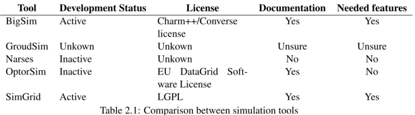
Where a small comparison between the tools is made. The table 2.1shows a comparison of the tools.
Tool Development Status License Documentation Needed features BigSim Active Charm++/Converse
license
Yes Yes
GroudSim Unkown Unkown Unsure Unsure
Narses Inactive Unkown No No
OptorSim Inactive EU DataGrid Soft-ware License
Yes No
SimGrid Active LGPL Yes Yes
Table 2.1: Comparison between simulation tools
Tools with no recent developments were excluded (some of them have more than 10 years without updates). This excludes both Narses and OptorSim.
Tools with unknown or restricted licensing were also excluded from the tool list, excluding GroudSim and Narses.
Excluding GrouSim, Narses and OptorSim from the tools list only leaves BigSim and SimGrid as viable options.
Ultimately SimGrid was chosen to be used for the simulations because it has been proven to be accurate, scalable, has good documentation and is popular on the academic world.
Background
2.7
Available Energy Consumption Reporting Tools and APIs
Power API
Power API by Sandia Corporation is "a portable API for power measurement and control" [Cor14]. A reference implementation is provided ( [Cor16b]) and it is written in C++ and C languages with sources available. It is released under a special license but it has the source code freely available.
It has a broad scope and a portable API [Cor15c]. It provides the possibility to be extended, so that it supports other hardware.
Intel Power Gadget
Intel Power Gadget is a software tool designed to monitor the power usage of Intel Core processors (starting from the 2nd generation). It reads the MSR registers and allows the logging of power consumption over time for different components of the CPU package [Cor15a].
Intel micsmc utility
Intel micsim utility is a tool designed to "manage the Intel Xeon Phi power configuration and facilitate power measurements" [Cor15b]. This tool while accurate is limited in usefulness since it only works with the Xeon Phi family.
Pstate-frequency
Pstate-frequency is a tool designed to manipulate the Linux kernel intel_pstate CPU scaling driver, enabling the user to set the maximum and minimum frequencies of the CPU and enable or disable the Intel Turbo Boost feature [Yam].
NVIDIA Management Library
The NVIDIA Management Library (NVML) is a C based API for "monitoring and managing various states of the NVIDIA GPU devices" [Corc]. It’s a tool that only works on NVIDIA GPUs making it limited in usefulness.
NVIDIA System Management Interface
The NVIDIA System Management Interface is a utility that is based on the NVML explained earlier. This utility allows to get the CPU power consumption from some NVIDIA cards [Cord].
AMD CodeXL Profiler
The AMD CodeXL profiler is a utility that helps developers profile their code and provides power consumption values from some CPUs and GPUs [AMDc]. It should be noted that CodeXL is now open source (as of April 19, 2016) and is now part of GPUOpen [AMDb].
Background
2.7.1 Comparison between tools
All tools are somewhat limited in one way or another. Most of them have limited hardware support. This creates an additional overhead since the tools must be tested on every test platform. All of them rely on hardware built in functionally and unless a bug is present the same hardware results should be the same across various tools.
Power API was not chosen since it had to be integrated on the used application in test. Intel micsmc was not used since no Xeon Phi platform was available for testing. Both NVIDIA tools were not used since the available NVIDIA GPU doesn’t support power consumption reporting. AMD CodeXL doesn’t support the available hardware so it was also not used. Both Intel Power Gadget and Pstate-frequency utilities were used since they support the available hardware.
Background
Chapter 3
Methodology
3.1
Introduction
This chapter contains the used methodology. First the energy analysis is discussed followed by the directly related performance analysis. Then the chosen benchmarks are detailed but it should be noted that this was not the main focus of the thesis so its scope is rather narrow. Finally the simulated platform model is detailed along with the task graph model.
3.2
Power and Energy Analysis
In the previous chapter two methods of obtaining power and energy consumptions were discussed, the hardware and software methods.
Since the external hardware methods obtain either a global value (that might be influenced by different factors) or involve invasive hardware modifications, they will not be used. Also there is another issue with the external hardware method that is the need to communicate and log the data provided by the measurement equipment.
The method that utilizes internal hardware counters was chosen since the values provided offer "a good match" [RRS+14] between the obtained values measured with the hardware counters and by using a power meter on the power rails that feed the CPU. Using internal hardware counters also provides another benefit: the ease to obtain those values through software, for example by using the Power API, which is very important in a multi node system. Another benefit is that more detailed power consumption data can be obtained from Intel CPUs, since they are partitioned in different internal power planes that provide their power consumption independently from each other.
Another thing that must be considered is the so called Turbo Boost (Intel) or Turbo Core (AMD) and other similar boost technologies that attempt to increase the performance of the CPU or GPU if possible. One example is if only a CPU core is being used that core can use a higher clock and effectively speeds up what is running on the core in use.
Methodology
System Time The system time when this particular measurement was taken. RDTSC The TSC value, which is the number of cycles since CPU reset. Elapsed Time (sec) Time elapsed since the Intel Power Gadget tool was started. IA Frequency_0 (MHz) CPU Core frequency. If more than one core exists in the package,
this contains the average frequency of those cores. Processor Power_0 (Watt) Total CPU package power consumption.
Cumulative Processor En-ergy_0 (Joules)
Sum of the energy spent by the CPU package since the logging start.
Cumulative Processor En-ergy_0 (mWh)
IA Power_0 (Watt) CPU cores power consumption. (Also known as PP0) Cumulative IA Energy_0
(Joules)
Sum of the energy spent by the CPU cores since the logging start.
Cumulative IA Energy_0 (mWh)
GT Power_0 (Watt) Internal GPU power consumption. (Also known as PP1) Cumulative GT Energy_0
(Joules)
Cumulative energy spent by the internal GPU since the logging start.
Cumulative GT Energy_0 (mWh)
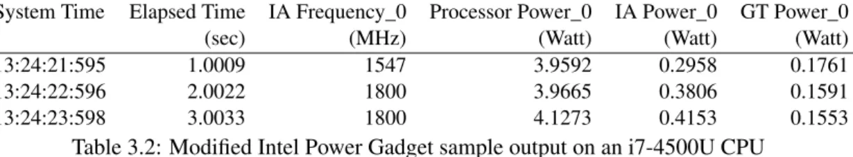
Table 3.1: Values provided on by the Intel Power Gadget on an i7-4500U
Another example is that not all tasks will make the CPU spend the same amount of power, if there is a power headroom the CPU might overclock itself to take advantage of this headroom. This technology has its benefits, but make the CPU or GPU performance more variable since this depends from many variables like temperature and current limits. When possible benchmarks with this technology enabled and disabled are performed and compared.
3.2.1 CPU
For CPU power consumption analysis the Intel Power Gadget for Linux was used. This tool enables easy logging various values obtained from the MSR registers from Intel CPUs (on Linux this requires that the msr kernel module to be loaded). Intel Power Gadget was chosen since only Intel CPUs were available for this work.
The Intel Power Gadget outputs a CSV file with the various values separated by time interval chosen by the user. A table explaining the obtained values from one of the test systems is provided, see3.1. The provided values vary from CPU to CPU (some Intel CPUs don’t have an integrated GPU for example). It should also be noted that if the computer system has more than one CPU this tool also provides the values for other present CPUs (eg multi socket workstations).
It should be noted that this output doesn’t match what was present in the documentation ana-lyzed in the previous chapter. There are no PP0 and PP1 values, in this case PP0 equals to IA, and PP1 equals to GT.
Methodology
System Time Elapsed Time IA Frequency_0 Processor Power_0 IA Power_0 GT Power_0
(sec) (MHz) (Watt) (Watt) (Watt)
13:24:21:595 1.0009 1547 3.9592 0.2958 0.1761
13:24:22:596 2.0022 1800 3.9665 0.3806 0.1591
13:24:23:598 3.0033 1800 4.1273 0.4153 0.1553
Table 3.2: Modified Intel Power Gadget sample output on an i7-4500U CPU
Since many of the outputs are not required, the Intel Power Gadget source code was modified to remove them. The RDTSC value and all cumulative values were removed. The cumulative values are then calculated using a spreadsheet according to the relevant time period in analysis. This was also required since some of the cumulative calculations were incorrect. The modified Intel Power Gadget results were validated against the non modified version as to make sure that no bugs were introduced.
To log the power consumption, the Intel Power Gadget is left running in the background and its output is stored to the computer storage in the form of a CSV file. The program reads the values each second.
A sample output from the modified Intel Power Gadget on one of the test systems is provided in the table3.2.
From this logs it is possible to get an insight on how much power the CPU consumes on a particular instant while executing different tasks. To calculate the energy consumption a simple calculation must be done, multiplying the power consumption average by the running time gives the spent energy in Joules.
3.2.1.1 CPU speed control
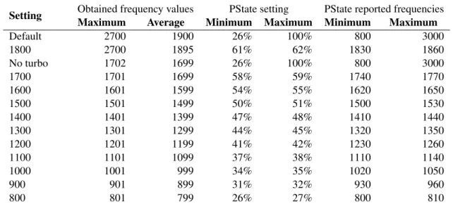
Due to time and hardware availability constrains only Intel CPUs will be used. Since the tested CPUs all use the Intel pstate Linux kernel driver, the pstate-frequency utility will be used to ma-nipulate the maximum and minimum frequencies. Since Intel uses SpeedStep (dynamic frequency scaling technology) the CPU clock frequency varies according to the load present on the CPU, this behavior will be studied when using the default CPU configurations.
Before running any benchmarks the possible frequency ranges are tested manually, since both the CPU or Intel pstate driver might ignore the defined frequency values (some frequencies steps might not be supported).
Then after obtaining the maximum and minimum percentage values required for the pstate-frequencyutility these are noted with the respective frequency. Doing this permits to know that the settings are really doing what they are supposed to do. This also has the added benefit of permitting scripting the frequency changes.
3.2.2 GPU
For GPU power consumption three tools were found: the NVIDIA System Management Interface one and Intel Power Gadget. AMD CodeXL profiler also reports AMD GPU power consumption.
Methodology
However on the available hardware none of them supported measuring power consumption for the dedicated GPU, only on the Intel integrated GPU was possible to measure power consumption.
3.2.3 GPU speed control
GPU speed control is not very different from the CPU speed control, but there are less power states to chose from. It is possible to change the running frequency of the GPU through some overclocking utilities but since the goal is not tweak each individual GPU (some GPUs even have this option locked) this will not be pursued.
NVIDIA has PowerMizer, a technology that automatically sets the power state according to the load imposed on the GPU. Some GPUs like the NVIDIA 980 GTX have 4 different performance levels and one boost state (similar in function to Intel Turbo Boost or AMD Turbo Core).
AMD GPUs also have multiple power states, for example the AMD R9 270X has 4 power states, a boost state is also provided (AMD PowerTune).
Intel integrated GPUs also have multiple power states, it should also be noted that they depend on the CPU load, since the TDP is shared between the CPU and GPU.
No research was made on AMD CPUs with integrated GPUs.
All analyzed manufacturers provide utilities to change the power settings, most of the times through performance profiles in the driver utility.
Methodology
3.3
Performance Analysis
In this section the benchmarks for performance analysis and their respective configurations will be discussed.
3.3.1 Chosen Benchmarks
3.3.1.1 Intel Optimized Linpack
Linpack was chosen since it measures how fast a system of linear equations of the type Ax=b can be solved by the computer system.
Since only Intel CPUs are being tested, using the Intel Linpack benchmark should take better advantage of the CPU instead of using a generic version of the benchmark. However it should be noted that this makes the comparison with other manufacturers CPUs invalid, since Intel does not "grantee the availability, functionality, or effectiveness of any optimization on microprocessors not manufactured by Intel" [Cora]. This should be taken in consideration for all benchmark utilities that are built using Intel Compilers.
Three configurations were made:
• Big: runs one test with problem size 20000. Chosen to simulate long jobs, avoiding job start and finish overheads (ex: memory allocations). The best results are expected in this test.
1 1 # number of tests
2 20000 # problem sizes
3 20000 # leading dimensions
4 4 # times to run a test
5 4 # alignment values (in KBytes)
Listing 3.1: Intel Linpack Big Configuration
• Small: runs one test with problem size 1000. Chosen to simulate small burst jobs, more overhead prone than the big test. Worse results are expected in this test.
1 1 # number of tests
2 1000 # problem sizes
3 1000 # leading dimensions
4 4 # times to run a test
5 4 # alignment values (in KBytes)
Listing 3.2: Intel Linpack Small Configuration
• Mixed: runs seven tests starting from 1000 to 20000 sizes. Includes both small and big tests, chosen to see the problem size effect of the obtained results.
Methodology
1 7 # number of tests
2 1000 2000 5000 10000 15000 18000 20000 # problem sizes
3 1000 2000 5000 10000 15000 18000 20000 # leading dimensions
4 4 4 4 4 4 4 4 # times to run a test
5 4 4 4 4 4 4 4 # alignment values (in KBytes)
Listing 3.3: Intel Linpack Mixed Configuration
All configurations run each test four times so that in the case an erroneous output is present (for example while Intel Turbo Boost is active) it can be discarded. For the output to be considered valid at least 3 outputs must be consistent (time and GFlops values must be within 5%).
3.3.1.2 High Performance Linpack for GPUs
This was chosen so that GPU performance would be obtained in a similar way of the CPU perfor-mance. It should be noted the previous benchmark and this one are not comparable since the code base and compiler are not the same.
No configurations were made since due to the lack of time and the non availability of built binaries this benchmark was not used.
3.3.2 Outputs
3.3.2.1 Intel Optimized Linpack
The Intel Linpack benchmark has two output values of interest: the time taken and the GFlops value. Listing3.4shows a snippet of the Intel Linpack output. This output shows that four 20000 problems were solved, each problem has its own time and GFlops value.
1 =================== Timing linear equation system solver ===================
2
3 Size LDA Align. Time(s) GFlops Residual Residual(norm) Check
4 20000 20000 4 99.032 53.8625 3.466513e-10 3.068624e-02 pass
5 20000 20000 4 105.277 50.6675 3.466513e-10 3.068624e-02 pass
6 20000 20000 4 105.131 50.7381 3.466513e-10 3.068624e-02 pass
7 20000 20000 4 104.774 50.9106 3.466513e-10 3.068624e-02 pass
Listing 3.4: Intel Linpack output snippet
The outputs are then imported to a spreadsheet so that they can be further processed.
Methodology
3.4
Simulated Platform Model
In this section the simulated platform model will be discussed. The utilized model is the SimGrid platform model but complemented since various shortcomings exist in it.
3.4.1 SimGrid Platform Model
SimGrid provides a platform model that is very network oriented, since it is not the goal of this dissertation to explore the networking aspect of SimGrid only a brief overview will be given.
While the SimGrid network modeling is very detailed, the actual computation modeling is not. This is an issue that will be discussed in3.4.2.
A sample SimGrid platform file is provided at the listing3.5. The provided sample describes a simple computer with a dedicated graphics card.
1 <?xml version=’1.0’?>
2 <!DOCTYPE platform SYSTEM "http://simgrid.gforge.inria.fr/simgrid/simgrid.dtd">
3 <platform version="4">
4 <AS id="AS0" routing="Full">
5 <host id="CPU0" speed="50Gf"/>
6 <host id="GPU0" speed="38Gf"/>
7 <link id="PEG0" bandwidth="2GBps" latency="10us" sharing_policy="FATPIPE" />
8 <route src="CPU0" dst="GPU0">
9 <link_ctn id="PEG0"/>
10 </route>
11 </AS>
12 </platform>
Listing 3.5: Sample SimGrid Platform file
3.4.2 SimGrid Platform Model limitations
SimGrid defines the entities that actually do the computation themselves as hosts. The hosts as defined in SimGrid 3.13 are very simple, they rely on a power value and a core count as far as performance is concerned.
No actual power values exist. This might create a slight confusion at first, since what SimGrid calls power is not at all related to energy and instead represents the number of flops that a host core can compute. A problem arises with using flops as a performance measure unit, running on the same exact hardware different programs that do exactly the same (eg multiplying two matrices) may yield very different flops performance values.
The core count has recently added to SimGrid (added on version 3.13) and it is not yet val-idated. SimGrid assumes that if 4 cores are present, 4 tasks can be executed without interfering with each other what is not true, there are a lot of factors that influence this.
Methodology
Factors such Intel Power Boost, TDP limits, cache access patterns, memory access times among many others influence the obtained performance.
With this in mind the SimGrid core count cannot be utilized due to the numerous issues that arise from using it (the speed value just gets multiplied by the core count).
SimGrid also ignores the architecture kind of the processing unit, so that, for example, a GPU cannot be distinguished from a CPU. This is very problematic since not all tasks can run on all architectures and task performance varies widely in different architectures. Since this dissertation needs to consider heterogeneous systems this is a problem that needs to be solved.
Another issue is the lack of power states. Nowadays many processing units have different power states with different performances. Since one of the goals of this dissertation is to be energy aware this is another problem that needs to be solved.
With this in mind SimGrid needs to be complemented as to better understand the underlying platform that it is simulating.
Methodology
3.5
Task Graph Model
In this chapter the chosen task graph model will be explained. As the basis of the task graph is a directed acyclic graph, more commonly known as a DAG. No further details will be given since this already discussed in chapter2.
3.5.1 SimGrid Task Model
SimGrid tasks are defined as jobs, they contain an unique identifier (id), a name-space and finally a name. Before going in to more detail it should be noted that valid DAX files are not accepted by SimGrid and that the provided examples fail to validate against the defined xml schema.
As far as computation time estimation they contain a runtime number that corresponds to the time it takes do complete the task on a host running at 4.2GFlops. This might pose a problem since it is assumed that the timings were made on a 4.2GFlops host for that particular task. Since different tasks behave differently on different platforms this is a dangerous assumption to make, with this in mind extra care will be taken dealing with this question.
Each task can have outputs and inputs from/to other tasks, each of them is represented on a separate uses tag. The link parameter defines if it is an input or an output. Also of hight importance is the size of the data to be transfered since that value is utilized to calculate the data transfer time.
3.5.2 SimGrid Task Graph Model
SimGrid uses a non standard DAX file as mentioned before. It focuses in the task description, the edges are obtained from the tasks themselves instead of being explicitly declared. A sample DAX is provided in the listing3.6, this is a very simple example with three sequential tasks.
Since SimGrid doesn’t allow modifications to the DAX file, all the required additions will be stored in a separate file, this is explored in detail in chapter4.
1 <?xml version="1.0" encoding="UTF-8"?>
2 <adag xmlns="http://pegasus.isi.edu/schema/DAX" xmlns:xsi="http://www.w3.org/2001/ XMLSchema-instance" xsi:schemaLocation="http://pegasus.isi.edu/schema/DAX http ://pegasus.isi.edu/schema/dax-2.1.xsd" version="2.1" count="1" index="0" name=" test" jobCount="3" fileCount="0" childCount="20">
3
4 <job id="ID00000" namespace="Test" name="T1" version="1.0" runtime="15">
5 <uses file="input_0" link="input" register="true" transfer="true" optional="false" type="data" size="10"/>
6 <uses file="output_0" link="output" register="true" transfer="true" optional="false " type="data" size="10"/>
7 </job>
8 <job id="ID00001" namespace="Test" name="T2" version="1.0" runtime="4">
9 <uses file="output_0" link="input" register="true" transfer="true" optional="false" type="data" size="10"/>
Methodology
10 <uses file="output_1" link="output" register="true" transfer="true" optional="false " type="data" size="10"/>
11 </job>
12 <job id="ID00002" namespace="Test" name="T3" version="1.0" runtime="1">
13 <uses file="output_1" link="input" register="true" transfer="true" optional="false" type="data" size="10"/>
14 <uses file="output_2" link="output" register="true" transfer="true" optional="false " type="data" size="10"/> 15 </job> 16 17 <child ref="ID00001"> 18 <parent ref="ID00000"/> 19 </child> 20 <child ref="ID00002"> 21 <parent ref="ID00001"/> 22 </child> 23 </adag>
Listing 3.6: Sample DAX
In the DAX file tasks are represented by job tags and relationships between tasks are described by child tags (see the edges section).
The job attributes are listed in the table 3.3 with a short description of what they are. All attributes are mandatory.
Attribute Description
id Job (task) id.
namespace Current task name space. name Task name.
version Needs always to be "1.0", has no importance for the simulation. runtime Task execution time in seconds to execute on a 4.2 GFlops host.
Table 3.3: DAX job tag attributes
Edges are not directly described by the DAX file format, but are represented in the nodes themselves through the file attribute on each node. Both inputs and outputs are possible in each node, so to create an edge between two nodes the output of the source node must be the input of the destination node and this relationship must be represented by a child tag. The uses tag attributes are listed in table3.4.
3.5.3 SimGrid Task Graph Model limitations
Not as bad as the platform model, the task graph model still has some limitations. The most impor-tant being the lack of platform awareness. With this in mind the task graph will be augmented so that platform awareness can be used, so that the supported platforms are known and the hopefully best platform can be recommended.
Methodology
Attribute Description
file File name.
link Defines if the file is an input or output.
register Boolean defining whenver the file is registered on a replica catalog. transfer Boolean defining whenever the result should be transmitted or not. optional Boolean defining if the file is optional.
type Defines the type of the output.
size Data size for transmission calculations Table 3.4: DAX file tag attributes
Two test DAGs will be created and other already existing DAGs will be used to test the schedul-ing algorithm.
3.5.4 Contech
Since its very useful to use real task graphs without having to make them manually, the Contech framework by Railing, Brian P. and Hein, Eric R. and Conte, Thomas M. will be analyzed.
Methodology
Chapter 4
Scheduler
4.1
Proposed Algorithm
4.1.1 Introduction
In this section the implemented scheduler algorithm will be discussed. Since it is based on the HEFT algorithm with minor changes, a brief overview of the HEFT algorithm is given first. Then the implemented scheduler is detailed.
4.1.2 HEFT Algorithm
The HEFT (or Heterogeneous Earliest Finish Time) is a scheduling algorithm proposed by Topcuoglu et al. It is described in conjunction with the CPOP algorithm [THW02]. In the algorithm 1the original pseudo code as proposed by Topcuoglu et al is transcribed.
The EFT value is calculated using the equation4.1.
EFT(ni, pk) = StartTime(ni, pk) + ExecutionTime(ni, pk) (4.1)
Algorithm 1 HEFT scheduling algorithm.
1: Set the computation costs of tasks and communication costs of edges with mean values.
2: Compute rankufor all tasks by traversing graph upward, starting from the exit task.
3: Sort the tasks in a scheduling list by non increasing order of rankuvalues.
4: while there are unscheduled tasks in the list do
5: Select the first task, ni, from the list for scheduling.
6: for each processor pkin the processor-set (pk∈ Q) do
7: Compute EFT (ni, pk) value using the insertion − based scheduling policy.
8: end for
9: Assign task ni to the processor pj that minimizes EFT of task ni.
Scheduler
4.1.3 HLEC Algorithm
The implemented scheduling algorithm is based on the HEFT algorithm. Two modifications were made to the algorithm.
The first modification was to make HEFT platform aware, ie: distinguish between a GPU and a CPU. This is important since each task must only be scheduled in the platforms that are supported by it.
The second modification was to change the EFT (Earliest Finish Time) to LEC (Lowest Energy Cost). This change was made so that instead of preferring the fastest execution time, the lowest energy consumption is preferred. With this modification the algorithm name became HLEC.
The modified pseudo code can be seen in the algorithm2.
The equation4.2shows how the LEC value can be calculated, by minimizing the LEC value the best host in terms of power consumption will be selected.
LEC(ni, pk) = EnergySpentSoFar(pk) + EnergyRequired(ni, pk) (4.2)
In the implementation the utilized equation4.3is not the same as the equation4.2, since due to the way that SimGrid works it was not possible to properly calculate the power consumption of a host so far, with this in mind the equation was changed to assume that the host was always in use before. See the chapter6for more details.
LEC(ni, pk) = Power(pk) ∗ (StartTime(ni, pk) + ExecutionTime(ni, pk)) (4.3)
Algorithm 2 Modified HEFT scheduling algorithm (HLEC).
1: Set the computation costs of tasks and communication costs of edges with mean values.
2: Compute rankufor all tasks by traversing graph upward, starting from the exit task.
3: Sort the tasks in a scheduling list by non increasing order of rankuvalues.
4: while there are unscheduled tasks in the list do
5: Select the first task, ni, from the list for scheduling.
6: for each processor pkin the task compatible processor-set (pk∈ QT ) do
7: Compute LEC(ni, pk) value using the insertion − based scheduling policy.
8: end for
9: Assign task nito the processor pjthat minimizes LEC of task ni.
10: end while
Scheduler
4.2
Implementation
In this section the scheduler implementation will be discussed. The code will not be explained in detail since the developed program is somewhat large.
4.2.1 Program structure
The program was initially built using the C language due to compatibility issues while linking the SimGrid library with the C++ based application. During the development process SimGrid 3.13 was released and fixed the C++ compatibility problem, so the program was ported to C++ in order facilitate the development process.
After testing the new library version it was obvious that some methods were missing. Those methods were added to the program itself so that no unnecessary modifications to the SimGrid code were done.
A object oriented approach was utilized, with this the program was separated in different classes.
There are 6 different parameters defined in this file.
1. PowerState Contains the power state information, including frequency and power rating. 2. AttributeHost Contains all the additional host attributes not supported by SimGrid. 3. AttributeTask Contains all the additional task attributes not supported by SimGrid. 4. Config Class with static variables containing the program configuration.
5. Output Class with static methods that provide scheduling result output, supporting CSV, Jedule and console output.
6. Scheduler The most important class: contains the scheduler, contains the implemented al-gorithms (HEFT and HLEC) and all auxiliary methods required.
7. Simulation Wrapper for the simulation, responsible for initializing the simulation environ-ment and loading the task graph and platform files.
Scheduler
4.3
Input Files
In this section the input files that the implemented scheduler uses are described.
4.3.1 Configuration Files
The developed application needs two configuration files, the global configuration file and the input configuration file. Both are detailed bellow.
4.3.1.1 Global configuration file
This file stores global configurations common to all possible inputs (nothing directly affects the simulation). It’s name must be config.json and must be on the DAG_Scheduler binary folder. The default configuration file is shown in the listing4.1.
1 { 2 "DAG_Scheduler_params": [{ 3 "platformsDir": "platforms/", 4 "platformAddonsDir": "platforms_addon/", 5 "daxDagsDir": "dax_dags/", 6 "daxDagAddonsDir": "dax_dags_addon/", 7 "outputDir": "scheduler_output/" 8 }] 9 }
Listing 4.1: Default config.json
The file is self explanatory and since it is not relevant for anything other than the initial con-figuration it will be not detailed any further.
4.3.1.2 Input configuration file
This file defines the inputs that the program will use. It defines what platform and graph files to load and the settings for the scheduler.
A sample input file is show in the listing4.2
1 { 2 "DAG_Scheduler_inputs": [{ 3 "platform": "S440.xml", 4 "daxDag": "CyberShake_100.xml", 5 "algorithm" : "LEEC", 6 "powerBudget": 60, 7 "useFastestSpeed" : false, 8 "speedThresholdPercent" : 60 9 }] 10 } 30
Scheduler
Listing 4.2: Sample input.json There are 6 different parameters defined in this file.
1. platform The platform file to load. 2. daxDag The graph file to load.
3. algorithm The algorithm to use, both LEC and HEFT are valid options here.
4. powerBudget The power budget in watts. This is currently ignored, see further work. 5. useFastestSpeed Boolean that determines if the highest performing power state is selected
or the optimal power state is selected.
6. speedThresholdPercent Integer that must be within 1 and 100 that defines the minimum power state possible.
If no parameter is passed the program will attempt to use a input.json file in the program folder, if passed it will use that file instead. This is used for scripting.
4.3.2 Graph
Here the two files required for the graph to be loaded will be discussed. Two files had to be used since SimGrid doesn’t allow any extra fields on the DAX file (as of SimGrid 3.13 if any extra field is found, the graph loading is aborted and exit is invoked killing the application).
The first file is the DAX graph that is widely used in many examples, it was chosen since its more complete and easy to work with than the other SimGrid supported (dotty) format. It should be noted that the DAX file format as used by SimGrid fails the XML Schema (XSD) Validation, so it is not standard and it’s compatibility with other software is unknown to the author.
The second file is a complementary file that stores extra parameters needed for the developed scheduler. This file uses JSON to store extra fields. With this approach no SimGrid code had to be modified and the original DAX files can be used with the oficial SimGrid version and other tools that support it since it still respects its original specifications.
4.3.2.1 DAX File
This file defines the task graph, it contains all the nodes (tasks) and edges (dependencies).
4.3.2.2 JSON File
In this file each node (task) must have an entry with the required extra fields. In the JSON file all extra attributes are defined, all nodes in the DAX file must also be present in this file (if using an extra JSON file at all). This works as a complement to the DAX file.
Scheduler
The extra job attributes are listed in table4.1with a short description of what they are, again all atributes are mandatory.
Attribute Description
jobID Job (task) id, must match a job ID in the DAX file. preferedPlatform Preferred platform for the task execution.
supportedPlatforms An JSON array of the supported platforms for the task to execute. Table 4.1: JSON job attributes
4.3.3 Platform
As on the graph two files are required. Once again the reason is the same from above (prevent SimGrid source code modifications and loss of compatibility).
The first file is the platform definition that SimGrid supports.
The second file is a complementary file that stores extra parameters that are required for the developed scheduler. As before JSON was chosen as the file format.
4.3.3.1 XML File
The XML file describes the platform that SimGrid will simulate. A more detailed description of this platform file is available in the SimGrid documentation. One thing that must be noted is that the host speed value defined on this file is ingnored since it is calculated from the complementary JSON file.
4.3.3.2 JSON File
In this file the extra fields for the platform are defined. All existing platforms on the XML file must also be present on this file. The most important fields present in this file are the idlePower and the powerStates. Without these fields it would be impossible to calculate power consumption values. The powerStates are also used to find the best operating point for that element in the platform. Table4.2contains all possible attributes.
Attribute Description
hostID Host id, must match a host ID in the xml platform file. platform Platform kind (CPU, GPU, etc..)
vendor Vendor name (AMD, Intel, NVIDIA, etc..) model Model name
coreCount Core count. Does not include logical cores (Hyper-threading, etc..) idlePower The power spent in idle by the host in watts.
maximumPower The maximum power that the host can drawn in watts. frequencyToGFlop The approximated frequency to flops ratio.
powerStates A json array of power states, consisting in id, power and frequency. Table 4.2: JSON host attributes
Scheduler
A simplified example can be seen at listing4.3, only one power states is shown.
1 { 2 "platform_attributes": [{ 3 "hostID": "CPU0", 4 "platform": "CPU", 5 "vendor": "Intel", 6 "model": "i7-4500U", 7 "coreCount": 2, 8 "idlePower": 3.13, 9 "maximumPower": 16.0, 10 "frequencyToGFlop" : 0.028, 11 "powerStates": [{ 12 "id": "P00", 13 "power": 7.14, 14 "frequency": 800 15 }, { 16 ... 17 } 18 }] 19 }
Scheduler
4.4
SimGrid library modification
As to avoid modifications in the SimGrid library code when possible new methods were written and called by the developed program. But since SimDag has some methods that are very difficult to override like the scheduling function, one modification had to be made.
4.4.1 Host speed change in runtime
Due to the way that SimGrid works, the host speed needed to be modified in runtime. The problem was that SimGrid gets the speed from the platform xml file and doesn’t provide methods to change the speed. As to keep compatibility the fastest speed should be set on the original xml file, but this is not required since the developed program ignores this value and calculates it from the json file values.
At least as of SimGrid 3.13 that is not possible, so the SimGrid library needed to be modified in order to support this. Since SimGrid is an open source project the source code was modified by the author. The modification can be found in the appendix.
4.5
Conclusions
Many low level details are omitted, since in order to comprehend the scheduler most of the devel-oped code is not required to be understood.
However some difficulties arose during the implementation phase, either by the lack of docu-mentation or due to the way that the SimGrid was programed.
Chapter 5
Results
In this chapter the obtained results are discussed.
5.1
Task Graph
Before starting with the scheduler development it was analyzed if it was feasible to generate task graphs using already existing tools.
5.1.1 Contech
The only analyzed tool was Contech. The code is available online [Rai], and was downloaded and compiled by the author. However since it was unusable at the time when it was tested by the author (either by some issue with the author setup or by some issue with the tested version).
Issues with the build system were fixed and the tool was built, however when attempting to profile a simple program it failed to produce a usable output. With this in mind it was discarded.
Due to time that it took to rebuild every time a fix was made the author ended spending more time than expected and no other tool was analyzed.
5.1.2 Existing examples
Many examples of task graphs in the DAX format were found. Some were used to test the sched-uler, but since there was no information on what platform the code ran they are only used to test the scheduler while ignoring all platforms differences.
5.1.3 Manually created
In order to test the additions to the DAX task graph two task graphs were created manually. One with three sequential tasks and another with a parallel task section.
Results
5.1.4 Simulation Results
The obtained results from the simulation are shown here, all simulations used the same platform configuration.
Due to the size of the utilized task graphs only the scheduling output from the created task graphs will be shown.
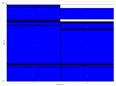
On figure5.1 the sequential test can be seen and on figure5.2 the parallel test can be seen (since both have the same result either using HEFT or HLEC, so only the HLEC result is shown). The processor 0 is the CPU and 1 is the GPU.
Figure 5.1: Sequential Test HLEC scheduler result
Figure 5.2: Parallel Test HLEC scheduler result
Results
Since the previous graphs had the same result using both algorithms, another graph was se-lected to highlight the main difference between both algorithms. The HEFT scheduler result is presented in the figure5.3, and the HLEC in5.4.
Since HLEC main goal is to save energy it will attempt to avoid using the dedicated GPU in the test platform and since the dedicated GPU idles at 0 watts this ends up saving energy, once again at the expense of worse runtimes.
Figure 5.3: Montage 100 HEFT scheduler result
Figure 5.4: Montage 100 HLEC scheduler result
Results
5.1.5 Comparison between HEFT and HLEC algorithms
Here the obtained results will be discussed. Before comparing results it should be noted that the HEFT algorithm has the platform awareness modification, since without it the results can not be compared.
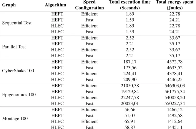
From the table5.1 it is possible to see that enabling the efficient speed configuration makes both algorithms spend less energy at the expense of runtime.
Graph Algorithm Speed Total execution time Total energy spent Configuration (Seconds) (Joules)
Sequential Test HEFT Efficient 1,89 22,78 HEFT Fast 1,59 24,21 HLEC Efficient 1,89 22,78 HLEC Fast 1,59 24,21 Parallel Test HEFT Efficient 2,52 33,67 HEFT Fast 2,21 35,17 HLEC Efficient 2,52 33,67 HLEC Fast 2,21 35,17 CyberShake 100 HEFT Efficient 187,17 4572,78 HEFT Fast 173,56 4633,52 HLEC Efficient 224,41 4378,41 HLEC Fast 209,90 4446,25 Epigenomics 100 HEFT Efficient 21050,38 546303,03 HEFT Fast 19129,84 561775,34 HLEC Efficient 22247,78 540058,20 HLEC Fast 20023,01 550227,34 Montage 100 HEFT Efficient 56,66 1466,12 HEFT Fast 51,07 1492,58 HLEC Efficient 65,91 1412,64 HLEC Fast 58,87 1445,11
Table 5.1: Scheduler time and energy outputs
Using the HEFT algorithm on the fast configuration as a baseline, it is possible to compare the different algorithm configurations on figure5.5.
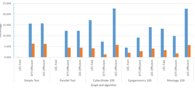
In this graph the configurations are grouped for each of the 5 different graphs, since the HEFT algorithm on the fast configuration was used as baseline it doesn’t appear in the graph as its values would always be zero. For each configuration two bars exist, one with the percentage of energy saved and another with the percentage of increased runtime. For example on the Montage 100 graph it is possible to see that the LEC-Efficient configuration there was a 22,7% increase in runtime and a 5.8% decrease in energy consumption.
Results
Figure 5.5: SimGrid Runtime vs Energy results
It is possible to conclude that the HLEC algorithm most of the times reduces the energy spent while doing the same tasks as the HEFT algorithm, also it is possible so see that by reducing the platform CPU speed the runtime increases but the spent energy decreases.