UNIVERSIDADE DE LISBOA FACULDADE DE CIÊNCIAS
DEPARTAMENTO DE BIOLOGIA ANIMAL
Relationships between the structure of sublitoral
assemblages and habitat complexity in a rocky shore
in the Portuguese coast
DANIEL FRIAS DE BARROS LOPES PINTO MESTRADO EM ECOLOGIA MARINHA
UNIVERSIDADE DE LISBOA FACULDADE DE CIÊNCIAS
DEPARTAMENTO DE BIOLOGIA ANIMAL
Relationships between the structure of sublitoral
assemblages and habitat complexity in a rocky shore
in the Portuguese coast
Dissertação orientada por: Professor Doutor Henrique Cabral
Professora Doutora Ana Silva
DANIEL FRIAS DE BARROS LOPES PINTO MESTRADO EM ECOLOGIA MARINHA
i Agradecimentos
Gostaria de agradecer ao Professor Doutor Henrique Cabral e à Doutora Ana Silva por terem aceite a orientação da minha tese de mestrado, bem como pelo apoio e ajuda que me deram ao longo de todo o processo.
Gostaria também de agradecer em geral à equipa de investigação do Professor Doutor Henrique Cabral por todo o apoio, e em especial à Sofia Henriques e ao Miguel Pais pelo importante contributo logístico que deram nas saídas de campo. Ainda dentro da equipa de investigação não poderia de deixar o meu profundo agradecimento à Inês Cardoso e à Joana Oliveira pela sua paciência, dedicação e fundamental ajuda que me deram, quer na parte das identificações quer na parte da escrita. Muito obrigado, este trabalho também é vosso.
Queria agradecer aos meus pais por toda a ajuda, compreensão e incondicional apoio, sem o qual este trabalho não teria sido possível. Obrigado por tudo o que significam para mim e por saber que vos tarei sempre ao meu lado.
Um grande obrigado também a ti Lucía pelo teu apoio e por teres estado nos bons e maus momentos e teres aguentado estes momentos mais complicados que nos apareceram à frente, mas que soubemos ultrapassar juntos. Sem ti tudo teria sido mais difícil.
Como não podia deixar de ser um grande obrigado a todos os que contribuíram directa e indirectamente para esta tese bem, como à minha família e amigos, espalhados pelo Algarve, Évora, Lisboa e alem fronteiras.
ii Finalmente não só a um agradecimento como também uma dedicatória: a ti Nuno, que onde quer que estejas, continuas a inspirar-me e a orgulhar-me. A tua memória está bem entregue. Obrigado por tudo.
iii Resumo
As zonas marinhas costeiras são áreas com um elevado interesse ecológico e biológico, desempenhando diversas funções, algumas das quais de extrema importância para a população Humana, como económicas ou de lazer. Ao longo da história da humanidade que se têm presenciado inúmeras migrações para estas zonas, bem como a criação de grandes aglomerados populacionais. Nas últimas décadas têm-se vindo a verificar um aumento das pressões antropogénicas nestas zonas, as quais têm contribuindo para a sua degradação ambiental e por sua vez, comprometendo as suas funções ecológicas e de funcionamento.
Entre as comunidades biológicas presentes nas zonas costeiras, destacam-se as dos invertebrados bentónicos. Estes organismos encontram-se na base das cadeias tróficas das comunidades, revelando-se assim de elevada importância ecológica. Estas espécies são também utilizadas como indicadores da qualidade ecológica da água devido algumas características particulares como sua baixa mobilidade, o seu curto ciclo de vida e a sua elevada sensibilidade a perturbações, fazendo desta forma que seja uma possibilidade viável para a monitorização da qualidade da água, e levando inclusive que estes organismos sejam inseridos em diversas metodologias científicas. As comunidades de invertebrados bentónicos são influenciadas por diversos factores, tais como a temperatura, exposição ao hidrodinâmismo e a complexidade topográfica do habitat. A maior complexidade do habitat parece estar relacionada com uma maior abundância e diversidade de taxa. Segundo alguns autores, algumas das razões que podem levar a uma maior abundância, podem estar relacionados com a maior disponibilidade de substrato, a protecção do hidrodinâmismo ou de potenciais predadores. A sazonalidade também é um factor modelador das comunidades bentónicas, no sentido em quanto mais severas as condições, neste caso fruto das estações do ano e suas características climatéricas
iv (menor luminosidade e temperatura e um aumento da turbidez e turbulência), menor vai ser o sucesso das comunidades bentónicas teoricamente.
O conhecimento científico existente para a costa portuguesa sobre as comunidades bentónicas de habitat rochoso é escasso, em particular no que se refere à relação a diversidade de taxa e a complexidade do habitat.
O presente trabalho teve como principal objectivo comparar as comunidades bentónicas de habitats rochosos com dois níveis de complexidade topográficas diferentes, em duas épocas do ano (Verão e Outono), com o propósito de verificar se a diferentes abundâncias e diversidade nos dois tipos de habitat se verificam independentemente ou não da sazonalidade e tentar compreender melhor estes factores modeladores das comunidades bentónicas. O estudo decorreu na costa marinha do Concelho de Cascais, em dois locais: Avencas, onde o substrato apresenta uma baixa complexidade estrutural, e na Guia, correspondendo a um substrato de elevada complexidade estrutural. As comunidades bentónicas foram amostradas através de duas abordagens distintas: com recurso a raspagens e a censos visuais, ambas realizadas em mergulho com escafandro autónomo. As raspagens foram efectuadas em unidades de substrato com 20 cm x 30 cm, tendo-se conservado o material recolhido em formol a 4% e crivado a 500µ, sendo posteriormente identificados em laboratório através de guias de identificação apropriados. Os censos visuais foram realizados com recurso a um quadrado de 50 cm x 50 cm, com 49 intersecções, equitativamente espaçadas, tendo-se registado cada espécie que coincidisse com os pontos de intersecção. A amostragem ocorreu em duas estações do ano, com a recolha de 24 replicados no mês de Agosto e 24 replicados no mês de Novembro, sendo 12 de uma zona topograficamente simples e 12 de uma topograficamente complexa.
v No total foram amostrados 27562 indivíduos e 188 espécies através da metodologia das raspagens, e um total de 3025 indivíduos e 30 espécies através da metodologia dos censos visuais.
Os resultados obtidos indicaram que as duas metodologias providenciam informação relativa a diferentes escalas espaciais, que afectam os padrões de distribuição e abundância das comunidades bentónicas. As diferentes escalas verificadas ficaram a dever-se principalmente a características de mobilidade e tamanho dos indivíduos. A PERMANOVA evidenciou a sazonalidade como factor estruturante. O efeito da complexidade do habitat só se revelou significativo quando em interacção com a sazonalidade. Foi igualmente possível identificar padrões de variação sazonal da abundância das espécies mais representativas em função da complexidade do habitat na análise SIMPER e na ordenação por escalamento multidimensional (MDS). No geral, verificou-se uma maior abundância no Verão e nos habitats de maior complexidade. No Outono, verificou-se que as associações de habitats de maior complexidade apresentaram maior homogeneidade. As diferenças de homogeneidade do verão para o inverno, possivelmente ficaram a dever-se ao facto de o verão coincidir tipicamente com a altura recrutamento. Uma vez que a maioria os organismos bentónicos apresentam normalmente uma estratégia de vida tipo r, ou seja apresentam um elevado número de indivíduos durante o recrutamento, mas também sofrem uma elevada mortalidade, possivelmente esta estratégia foi umas das causas que levou a verificar-se uma maior abundância e diversidade no verão e um visível decréscimo desta no inverno. No inverno o decréscimo da abundância e da biodiversidade foi mais visível nas zonas de habitat simples do que nas zonas de habitat complexo, possivelmente devido à protecção que estes oferecem dos factores bióticos e abióticos ao contrário das zonas de habitat simples. Também foi possível verificar que as comunidades formadas por organismos bentónicos livres
vi (recolhidos através de raspagens) apresentam uma variabilidade em relação ao habitat e à sazonalidade muito mais evidente que os organismos bentónicos fixos ao substrato (recolhido através do método dos censos visuais) onde os padrões não são tão evidentes, e quer o número de espécies, quer de abundância se mantêm mais uniformes ao longo da amostragem. Verificou-se igualmente a existência de padrões entre os taxas amostrados, onde algumas espécies foram mais abundantes dependendo de características da complexidade do habitat ou da sazonalidade. Os taxas Hiatella artica (Linnaeus, 1767), Alvania sp. (Risso, 1826), Tapes rhomboids (Pennant, 1777) e Ulva lactuca (Linnaeus, 1753) apresentaram maior abundância no Verão, enquanto que Spirobranchus lamarckii (Quatrefages, 1866), Musculus sp. (Röding, 1798), Ciocalypta penicillus (Bowerbank, 1862), Litophylum incrustans (Philippi, 1837) e Coralina enlogata (J. Ellis & Solander, 1786) registaram maior abundância no Outono. Relativamente à complexidade do habitat, os taxa Hiatella artica, Alvania sp., Coralina enlogata, Spirobranchus lamarcky, Litophylum incrustans, e Nereididae apresentaram valores de abundância mais elevados nas zonas de habitat com maior complexidade, enquanto que nas zonas de habitat simples, as espécies melhor representadas foram Ulva lactuca, Musculus sp. e Ciocalypta penicillus.
Através deste trabalho, foi possível ver que nestas condições a sazonalidade pareceu ter uma maior preponderância em relação às abundâncias relativas à complexidade do habitat. Uma das razões que pode ter contribuído para este padrão foi o facto de as áreas amostragens não terem dimensão suficiente para que não sejam influenciadas pela migração de outras áreas com características diferentes. Verificou-se igualmente que certas espécies são mais características quer do habitat complexo, quer do habitat simples. Como indicações para o futuro, seria importante a continuidade deste estudo, de forma a englobar as restantes épocas do ano e a verificar se a variabilidade
vii interanual é muito marcada. A incorporação das associações de invertebrados bentónicos em planos de monitorização é particularmente útil, inclusive num contexto de avaliação da qualidade ecológica das águas costeiras. Quanto maior o conhecimento das comunidades bentónicas e seus padrões, melhor e mais adequada resposta pode vir a ser dada para a preservação destas comunidades e consequentemente dos ecossistemas que delas dependem.
viii Summary
The benthic communities are influenced by different natural factors, such as habitat complexity and seasonality. Some authors describe that, the more complex the habitat, the higher the abundance and biodiversity by the taxa, and for the seasonal influence, generally the colder seasons are associated to a lower abundance and biodiversity by the taxa. The main objective of this present work was to evaluate the relation between the diversity and abundance of the benthic community in two different types of rocky habitat (of high and low topographic complexity) in the coastal zone of Cascais, and if the patterns were consistent independently from the season (summer and autumn). The sampling as conducted in Avencas (low complex habitats) and in Guia (high complex habitats), using SCUBA diving procedures and the methodologies of: biomass collection (21cmx30cm) and intersection points in a quadrate of 50x50cm, with equal grid space (49 intersections). The results showed that the seasonality, when compared with the habitat complexity appeared to have a higher influence in the benthic communities. The habitat complexity only was significant when associated with the seasonality. The majority of the taxonomical groups showed higher abundances in summer and in the high complex habitats. The results also showed that the two methods revealed information concerning two different spatial scales. We saw that in the biomass collection method, the main taxa sampled were the Bivalvia, Gastropoda, Malacostraca and Polychaeta. As for the main taxa sampled by the intersection point method, were Demospongiae, Florideophyceae and Ulvophyceae. In general the majority of the species were more abundant in the complex habitats, but in most of the cases the differences weren’t as large as expected. As for the seasonality factor, it didn’t seem to have global tendency.
Keywords: benthic communities, habitat complexity, rocky areas, seasonality, species richness.
Index Agradecimentos ... i Resumo ………..……… iii Summary ………..………. viii CHAPTER 1 General introduction ………. 2 References ………... 6 CHAPTER 2 Relationships between the structure of subtidal assemblages and habitat complexity in a rocky shore in the Portuguese coast. 1. Introduction ………..……….. 13
2. Material and methods ……… 2.1. Study sites ... 16
2.2. Sampling procedures ………... 17
2.3. Data analyses ……….………..…. 18
3. Results ... 3.1. Biomass collection method ... 19
3.2. Intersection points method ... 27
4. Discussion ... 35
References ... 40
CHAPTER 3 Final remarks ... 51
1
Chapter 1
General introduction2 General introduction
The coastal zones are one of the most productive marine systems in the world, causing, trough history, for large population agglomerates to migration and fixate around this areas, in order to benefit from it’s resources. The resources available from the marine coastal zones have different applications such as ecological, economical or recreation. These zones show a high ecological value because of the favorable conditions for the establishment of rich and diverse communities and, for providing nurseries areas for a large number of fishes (Warre et al., 2010). These characteristics result not only from topographic and light availability, but also due to other influences, such as the high levels of nutrients and organic matter that are introduced by the estuaries into the coastal habitats (Costa et al., 2007). Economically, they are very important once millions of people are dependent of its resources for food or business purposes (Worm et al., 2006), but can also be a source of entertainment and pleasure. The main threats for these marine coastal habitats, over the past decades, have resulted from anthropogenic pressures (Fraschetti et al., 2011) from different sources, such as contamination from groundwater, eutrophication, water pollution, sedimentation and habitat loss (Gordoa, 2009). The coastline dynamic has been also affected by anthropogenic influences such as the building of ports and marinas, leading for the alteration of its hydrodynamics and natural habitats, but little importance has been given to these pressures (Underwood & Chapman, 1999). Other factors affecting the marine communities include: overfishing (Jennings & Kaiser, 1998), invasive alien species (Bax et al., 2003), biological interaction (Sousa, 1984), and most recently, the effects of global climate change (Graham et al., 2003).
Given the vulnerability of this habitats and the high dependency of the human populations from them, some attempts to protect these zones have been made, namely trough the creation by Europe of the Water Frame Work Directive,
3 which aims to obtain a “good ecological status” for all waters in Europe, including transitional waters by 2015 (EEC, 2000; Logan & Furse, 2002), or in the north America the Manguson-Stevens Fishery Conservation and Management Act whose objective is to achieve the conservation and management of fisheries levels (U.S. Department of commerce, 2007).
In these marine habitats, we can find different trofic chains, but all of them have benthic organisms in the bottom of the chain, causing them to be key and vital organism in any community richness and biodiversity (Bolam et al., 2002; Emmerson & Huxham 2002). The benthic species also contribute for the “cleaning” of the sea floor due to their capacity to process the particulate, organic materials (detritus and small organisms) that are deposited on the seafloor or that are suspended within reach of the organisms. This ability is applied by using a wide range of feeding strategies such as deposit feeding, suspension feeding, filter feeding, or scavenging (Burd et al, 2008).
Resulting from particular characteristics by the benthic communities such as a high sensibility to integrate changes in the sediments and water, limited mobility and to a short life cycle, they are used as sentinels for the water quality and causing their inclusion in diverse methodologies to test the water quality in different aquatic ecosystems (Orfanidis et al., 2003; Burd et al., 2008; Frontalin et al., 2009).
Inside of the coastal zones we can encounter distinct and characteristic types of habitats: the hard bottom (formed by static substratum) and soft-bottom habitats (formed by mobile substratum), being the soft-bottom far more common in nature (Gray, 1981). Soft-bottom habitats are typically characterized for being colonized mainly by polychetes, bivalves, molluscus, amphipods, decapods, crustaceans and echinoderms that generally have the ability to penetrate the substrate at different depths (Castelli et al., 2004). The hard-bottom habitats are characterized for having more sessile organisms with modular structure, such
4 as algae, cnidarians or bryozoans (Bianchi et al., 2004). To illustrate the importance of rocky habitats, nowadays virtually all marine protected areas are created in rocky habitats (Bianchi et al., 2004).
The rocky habitats communities are affected by several biotic factors, as competition, predation and recruitment success (Sousa, 1984; Dunstan & Johnson, 2003; Wernberg & Connell, 2008), and abiotic factors such as depth, turbulence, freshwater, salinity, light, seasonal variation and habitat complexity (Middelboe et al., 2003; Kostylev et al., 2005; Burd et al., 2008).
The habitat complexity, which is the main influence studied in this work, is well documented at different scales and in large number of habitats (McCormick, 1994; Kerr et al., 2001, Rahbek & Graves, 2001; Kelaher, 2003).
According to some authors larger biodiversity and abundance would be expected in the more complex habitats due to: higher availability of niches allowing different species to co-exist (Sousa 1984; Kostylev et al., 2005); the predators becoming less efficient (Russo, 1987; Diehl, 1988); higher possibility of refuges from physical and biological disturbance (Bergeron & Bourget 1986; Fairweather 1988); and because of the topographic complexity, the habitat works as a barrier for mobile dispersion (Erlandsson et al., 1999), making that immigration and emigration rates generally greater in simple surfaces when compared with complex habitats (Underwood & Chapman, 1989). According to Stål et al (2006), this tendency not only reflects on the benthic organism but also in different scales as fish communities, where the mean number of fish and biomass are higher on hard bottoms, as well as gastropods and amphipods. Also according to this author, the main fish species found on the hard bottom habitats are resident species, while temporary visitors dominate the soft bottom species.
Nowadays, there is an acceptable level of knowledge relative to the structure and the dynamic of the associations of benthic invertebrates in the marine rocky
5 habitats. Nevertheless the relation between the habitat complexity, the biodiversity and other structure characteristics of the marine communities are not well known for the Portuguese coast. On a more applied perspective, there have been several methodologies suggested to evaluate the ecological quality of the coastal zones, but these methodologies tend to forget the habitat complexity/structure.
6 References
Bax, N., 2003. Marine invasive alien species: a threat to global biodiversity. Mar. Policy, 27(4): 313-323.
Bergeron, P. & Bourget, E., 1986. Shore topography and spatial partitioning of crevice refuges by sessile epibenthos in an ice disturbed environment. Mar. Ecol. Prog. Ser., 28: 129–145.
Bianchi, C. N., Pronzato, R., Cattaneo-Vietti, R., Benedetti Cecchi, L., Morri, C., Pansini, M., Chemello, R., Milazzo, M., Fraschetti, S., Terlizzi, A., Peirano, A., Salvati, E., Benzoni, F., Calcinai, B., Cerrano, C., Bavestrello, G., 2004. Hard bottoms. Biologia Marina Mediterranea, 11: 185-215.
Bolam S. G., Fernandes T. F., Huxham M., 2002. Diversity, biomass, and ecosystem processes in the marine benthos. Ecol. Monogr., 72: 599–615. Burd, B. J., Barnes, P. A. G., Wright, C. A., Thomson, R. E., 2008. A review of
subtidal benthic habitats and invertebrate biota of the Strait of Georgia, British Columbia. Mar. Environ. Res., 66: 3-38.
Castelli, A., Lardicci, C., Tagliapietra, D., 2004. Chapter 4: Soft-bottom macrobenthos Biologia Marina Mediterranea, 11: 90-131.
Costa, M. J., Almeida, P. R., Cabral, H. N., Costa, J. L., Silva, G., Pereira, T., Rego, A., Azeda, C., Lopes, J. C., Tanner, S., Antunes, M., Batista, M., Baeta, F., 2007. Caracterização das comunidades de macroinvertebrados bentónicos e monitorização da qualidade ecológica da frente Atlântica do
7 concelho de Almada. Relatório Final. Instituto de Oceanografia da Faculdade de Ciências da Universidade de Lisboa, Lisboa, Portugal. Diehl, S., 1988. Foraging efficiency of three freshwater fishes: effects of
structural complexity and light. Oikos, 53: 207–214.
Dunstan, P. K., Johnson, C. R., 2003. Competition coefficients in a marine epibenthic assemblage depend on spatial structure. Oikos, 100(1): 79-88. EEC, 2000. Directive 2000/60/EC of the European Parliament and of the
Council of 23 October 2000 establishing a framework for Community action in the field of water policy. Off. J. Eur. Communities, 43: 1–72. Emmerson M. C., Huxham M., 2002. How can marine ecologists contribute to
the biodiversity ecosystem functioning debate? In: Loreau M, Inchausti P, Naeem S (eds) Biodiversity and ecosystem functioning: synthesis and perspectives, Oxford University Press, Oxford, pp: 139–146.
Erlandsson, J., Kostylev, V., Williams, G. A. 1999. A field technique for estimating the influence of surface complexity on movement tortuosity in the tropical limpet Cellana grata Gould. Ophelia, 50(3): 215-224.
Fairweather, P.G., 1988. Predation creates haloes of bare space among prey on rocky seashores in New South Wales. Aust. J. Ecol., 13: 401–409. Fraschetti,S., Guarnieri, G., Bevilacqua, S., Terlizzi ,A., Claudet, J., Russo, G.
8 biodiversity countdowns: what information do we really need? Aquat. Conserv. Mar. Freshwat. Ecosyst., 21(3): 299–306.
Gordoa, A., 2009. Characterization of the infralittoral system along the north-east Spanish coast based on sport shore-based fishing tournament catches. Est. Coast. Shelf Sci., 82(1): 41-49.
Graham, M. H., Dayton, P. K., Erlandson, J. M., 2003. Ice ages and ecological transitions on temperate coasts. Trends Ecol. Evol., 18(1): 33-40.
Gray, J. S., 1981. The ecology of marine sediments. Cambridge University. Cambridge, U. K. Press: 185 pp.
Jennings, S., Kaiser, M. J., 1998. The effects of fishing on marine ecosystems. Adv. Mar. Biol., 34: 201–352.
Kelaher, B. P., 2003. Changes in habitat complexity negatively affect diverse gastropod assemblages in coralline algal turf. Oecol. Aquat., 135(3), 431-41.
Kerr, J. T., Southwood, T. R., Cihlar, J., 2001. Remotely sensed habitat diversity predicts butterfly species richness and community similarity in Canada. Proceedings of the National Academy of Sciences of the United States of America, 98(20): 11365-70.
Kostylev, V., Erlandsson, J., Ming, M., Williams, G. 2005. The relative importance of habitat complexity and surface area in assessing biodiversity: Fractal application on rocky shores. Ecol. Complex., 2(3): 272-286.
9 Logan, P., Furse, M., 2002. Preparing for the European Water Framewor Directive? making the links between habitat and aquatic biota. Aquat. Conserv. Mar. Freshwat. Ecosyst., 12(4): 425-437.
McCormick, M., 1994. Comparison of field methods for measuring surface topography and their associations with a tropical reef fish assemblage. Mar. Ecol. Prog. Ser., 112(1981): 87-96.
Middelboe, A., 2003. Spatial and interannual variations with depth in eelgrass populations. J. Exp. Mar. Biol. Ecol., 291(1): 1-15.
Orfanidis, S., Panayotidis, P., Stamatis, N. 2003. An insight to the ecological evaluation index (EEI). Ecol. Indicat., 3(1): 27-33.
Rahbek, C., Graves, G. R., 2001. Multiscale assessment of patterns of avian species richness. Proceedings of the National Academy of Sciences of the United States of America, 98(8): 4534-9.
Russo, A., 1987. Role of habitat complexity in mediating predation by the gray damselfish Abudefduf sordidus on epiphytal amphipods. Mar. Ecol. Prog. Ser., 36(2): 101-105.
Sousa, W., 1984. Intertidal mosaics: patch size, propagule availability, and spatially variable patterns of succession. Ecology, 65: 1918–1935.
Stål, J., Pihl, L., Wennhage, H., 2007. Food utilisation by coastal fish assemblages in rocky and soft bottoms on the Swedish west coast: Inference for identification of essential fish habitats. Estuar. Coast. Shelf Sci., 71(3-4): 593-607.
10 Underwood, A. J., Chapman, M. G., 1989. Experimental analysis of the influences of topography of the substratum on movements and density of an intertidal snail, Littorina unifasciata. J. Exp. Mar. Biol. Ecol., 134: 175– 196
Underwood, A. J., Chapman, M. G., 1999. The role of ecology in coastal zone management: perspectives from south-east Australia. Perspectives on integrated coastal zone management. W. Salomons, R. K. Turner, L. D. de Lacerda and S. Ramachandran. Berlin, Springer: 99-128.
U.S. Department of commerce, 2007. Magnuson-Stevens Fishery Conservation and Management Act Public Law 94-265. National Oceanic and Atmospheric Administration National Marine Fisheries Service. U.S.A. Warren, M. A., Gregory, R. S., Laurel, B. J., Snelgrove, P. V. R., 2010.
Increasing density of juvenile Atlantic (Gadus morhua) and Greenland cod (G. ogac) in association with spatial expansion and recovery of eelgrass (Zostera marina) in a coastal nursery habitat. J. Exp. Mar. Biol. Ecol., 394(1-2): 154-160.
Wernberg, T., Connell, S., 2008. Physical disturbance and subtidal habitat structure on open rocky coasts: Effects of wave exposure, extent and intensity. J. Sea. Res., 59(4): 237-248.
Worm, B., Barbier, E. B., Beaumont, N., Duffy, J. E., Folke, C., Halpern, B. S., Jackson, J. B. C., Lotze, H. K., Micheli, F., Palumbi, S. R., Sala, E., Selkoe, K. A., Stachowicz, J. J., Watson, R., 2006. Impacts of biodiversity
11 loss on ocean ecosystem services. Science (New York, N.Y.), 314(5800): 787-90.
12
Chapter 2
Relationships between the structure of subtidal assemblages and habitat complexity in a rocky shore in the Portuguese coast.
13 1. Introduction
The benthic communities play an important role in the structure and functioning of coastal ecosystems due to their capacity to recycle nutrients and inorganic compounds, for their role as prey for top feeders and to their ability to create biogenic habitats (e.g. Warren et al., 2010). Marine benthic organisms are usually characterized by their limited mobility, short life cycle, and for their different sensibilities to integrate changes in the sediments and water, which have contributed for their use as important indicators of the habitat's health (e.g. Bilyard, 1987; Underwood, 2000; Silva, 2006).
Most studies on these communities were conducted in estuarine and marine coastal habitats. Among marine habitats, intertidal and subtidal areas have been frequently used to test ecological theories, and hard-bottom areas have been more often selected due to their higher biodiversity, in contrast with soft-bottom benthic communities (Bianchi et al., 2004).
Benthic communities are composed by sessil, sedentary or rooted organisms (Morri et al., 2004) and are affected by several biotic and abiotic factors. In the biotic factors, normally we can find competition among species, predation and recruitment success influence the biodiversity and abundance (Sousa, 1984; Underwood & Anderson, 1994; Maughan & Barnes, 2000; Dunstan & Johnson, 2003). Concerning abiotic factors examples, we have for instance the physical disturbances (e.g. wave action), that becomes usually less intense as depth increases, as well as the energy input for photosynthesis, affecting particularly algal assemblages and resulting in a marked reduction in species diversity as depth increases (Menconi et al., 1999; Middelboe et al., 2003). Turbulence, freshwater, salinity and, seasonal variation and habitat complexity that will be studied in the present work, are also examples of abiotic influences (Middelboe et al., 2003; Kostylev et al., 2005; Burd et al., 2008).
14 Seasonality is an important factor because of it’s capacity to affect different areas such as reproduction, recruitment and early colonization in the rocky habitats (Coma et al., 2000; Watson & Barnes 2004; Underwood & Chapman, 2006; Antoniadou et al., 2011), and adding temporal variability in resources and habitats (Ballesteros, 1991; Coma et al., 2000). The organism abundances also affect the environment: depending on the season there will be different algae abundances, leading to the variation on sediment accumulation (Kennelly, 1989), light levels (Gerard, 1984), recruitment, survival and growth of understory algae and invertebrates (Connell, 2003).
The influence of the habitat topographic complexity on species diversity and abundance, is well documented at different spatial and temporal scales (McCormick, 1994; Petren & Case, 1998; Kerr et al., 2001; Rahbek & Graves, 2001; Kelaher, 2003). This complexity can be increased by the colonization of organisms, such as barnacles or algae, which can influence the configurations and spatial patterns (Underwood & Chapman, 1989; Jacobi & Langevin, 1996; Templado et al., 2009). Structural complexity also increases the availability for settlement surface (Jacobi & Langevin, 1996), and provide refuge from predation (Johns & Mann, 1987; Russo, 1987; Diehl, 1988; Kenyon et al., 1995; Moksnes et al., 1998; Stunz & Minello, 2001), in fact, it has been demonstrated that the more complex the habitat, the less efficient are the predators (Russo, 1987; Diehl, 1988), resulting on an important mechanism to maintain the biological diversity. For this reasons, it is expected that the rocky habitats will have a wider number of species with abundances more stable, and having by far a higher ecological interest, when compared to the apparent uniformity of the soft bottom habitats (Bianchi et al., 2004)
Generally, species living in a more homogeneous habitat are more likely to migrate due to the lack of physical barriers, facilitating migration to complex
15 habitats (Sousa 1984; Underwood & Chapman, 1989; Jacobi & Langevin, 1996; Kostylev et al., 2005).
Nowadays, there is an acceptable level of knowledge relative to the structure and the dynamic of the associations of benthic invertebrates in the marine rocky habitats. Nevertheless the relation between the habitat complexity, the biodiversity and other structure characteristics of the marine communities are not well known for the south west Europe, particularly in the subtidal (Beldade, 1998; Boaventura, 1998). To fill this gap, the sampling site chosen was Cascais, which is characterized by a large extension of rocky habitats, creating a natural shelter that support a large number of marine biodiversity.
In order to study benthic invertebrates assemblages, the methodologies of semi-quantitative intersection points and quantitative biomass collection in a quadrate were performed. The aim of this study was to evaluate if the habitat complexity affected benthic assemblages, having as main hypothesis that, independently of the season, higher taxa richness and abundance were significantly associated to high complexity rocky habitats. With this information, biodiversity management frameworks will be likely to be more efficient and a database will be created for rocky shallow communities in the Cascais coast.
16 2. Material and methods
2.1. Study sites
This study was conducted in the West coast of Portugal (orientation WSW-ENE), nearby Cascais. This coastal area is protected from prevailing winds from the North. It is a typical limestone area (Saldanha, 1974; Ramalho et al., 2001), with a large variability of algae, fishes and invertebrates that depend on this area for shelter, reproduction and food supply (Cabral et al., 2010). The protection from the dominant hydrodynamic disturbance (northwest), allows the fixation of more sensible species (Cabral et al., 2010).
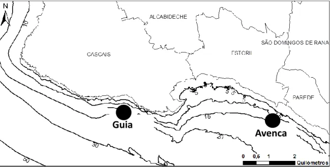
Two sublitoral rocky areas with different substratum characteristics were selected for this study: Avencas, because of its low complex habitats (38°41,06’N, 9°26,71’W), and Guia, where high complexity habitat were dominant (38°41,61’N, 9°26,71W) (Fig. 1).
Figure 1- Location of the sampling areas: Avencas (38°41,06’N, 9°26,71’W) and Guia (38°41,61’N, 9°26,71W).
Avenca
s
Guia
17 Habitat complexity was defined accordingly to the type of rock surface, based on Kostylev et al. (1996), Johnson et al. (2003), Ettema, & Wardle (2002) and Kostylev et al. (2005). Two categories were defined: high complex habitats locations were composed by irregular rocky platforms with high roughness and a large number of crevices; low complex habitats sites were composed by a series of smooth and flat rocky platforms.
2.2. Sampling procedures
Sampling took place in two sites in each sampling area (Avencas and Guia), in two dates, in two seasons, i.e. Summer (2 and 30 July 2010) and Autumn (4 and 31 October 2010), using SCUBA diving methodologies, at 5m depth in similar conditions of light (not shaded) and horizontality.
Two sampling methods were used. The first one consisted in quantitative biomass collection in quadrants measuring21cm x 30cm, that were scrapped to a sealed bag (Bianchi et al., 2004). The collected samples were preserved in 4% formalin and, at the laboratory, sieved trough 500 µm, and all the individuals identified to lowest taxonomic level possible and counted (Boaventura, 1996; Sconfietti et al., 2003; Bianchi et al., 2004, Marchini et al., 2004). Three replicates per sampling site and date were collected (48 samples in total). The second sampling technique was the semi-quantitative intersection point method, which consisted in the quantification of the macrobenthic organisms using a 50×50cm sampling quadrate with 49 intersections and equal grid space, whereby all organisms matching an intersection were identified and registered (Boaventura, 1996; Boaventura et al., 2002; Bianchi et al., 2004; Parravicini et al., 2009). Three replicates per sampling site and date were also collected (48 samples in total).
18 2.3. Data analyses
In order to balance the weight of dominant and rare species, the fourth root transformation was applied to all data. Differences in benthic assemblages were tested for the two sampling methods independently considering the following factors: season (Summer and Autumn), dates, habitat complexity (high and low) and location (nested within habitat complexity, with 2 levels: Guia 1, Guia 2, Avencas 1 and Avencas 2), using a PERMANOVA run on PRIMER+ software (Clarke & Warwick 2007, Anderson et al., 2008). The Bray-Curtis distance was used. The SIMPER method was applied in order to find out the main groups responsible for differences in benthic assemblages. This analysis used the similarity matrix calculated also using the Bray-Curtis distance. To detect the main ecological gradients a Multidimensional Scaling (MDS) was performed using the same data matrix.
19 3 Results
3.1. Biomass collection method
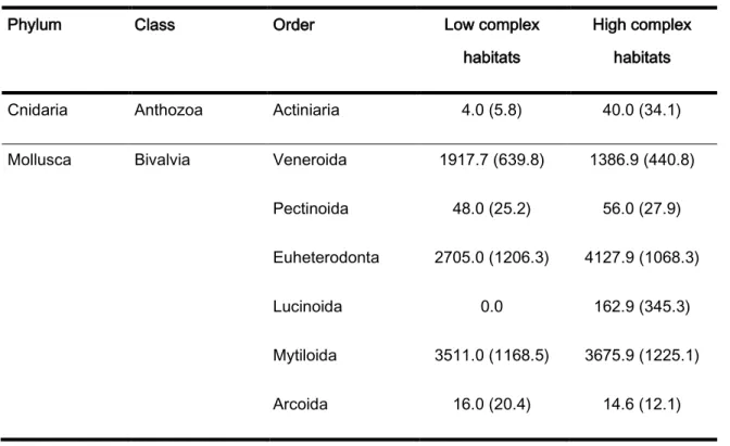
The highest number of individuals and taxa were observed in the biomass collection method, 27562 and 188, respectively. In the low complex habitats, the communities were mainly formed by Bivalvia (Veneroida, Mytiloida and Euheterodonta), Gastropoda (Littorinimorpha and negastropoda), Malacostraca (Amphipoda, Isopoda and Decapoda) and Polychaeta (Phyllodocida and Sabellida). As for the high complex habitats, they were mainly formed by Bivalvia (Veneroida, Pectinoida, Euheterodonta, Lucinoida and Mytiloida), Gastropoda (Littorinimorpha, negastropoda and Caenogastropoda), Polyplacophora (Lepidopleurida), Echinodermata, Malacostraca (Amphipoda, Isopoda and Decapoda), Maxillopoda (Sessilia) and Polychaeta (Phyllodocida, Eunicida, Spionida and Sabellida) (table 1).
Table 1: Mean densities (individuals/m-2) and its standard deviation of the taxas sampled by the biomass
collection method.
Phylum Class Order Low complex
habitats
High complex habitats
Cnidaria Anthozoa Actiniaria 4.0 (5.8) 40.0 (34.1)
Mollusca Bivalvia Veneroida 1917.7 (639.8) 1386.9 (440.8)
Pectinoida 48.0 (25.2) 56.0 (27.9)
Euheterodonta 2705.0 (1206.3) 4127.9 (1068.3)
Lucinoida 0.0 162.9 (345.3)
Mytiloida 3511.0 (1168.5) 3675.9 (1225.1)
20 Nuculida 0.0 4.0 (7.1) Myoida 6.0 (10.7) 0.0 Tanaidacea 0.0 2.6 (4.9) Gastropoda Littorinimorpha 2293.0 (1262.3) 2242.9 (508.9) Neogastropoda 196.9 (62.7) 231.7 (81.5) - 76.8 (47.6) 76.1 (43.5) Caenogastropoda 34.0 (24.3) 210.3 (133.0) Polyplacophora Chitonida 6.0 (8.3) 2.6 (4.9) Lepidopleurida 29.3 (19.4) 58.7 (29.9) Echinodermata Ophiuroidea - 31.3 (28.9) 16.6 (19.7) Echinodermata Camarodonta 0.0 2.6 (7.1) - 12.6 (22.3) 472.0 (884.7) Holothuroidea - 4.0 (7.8) 3.3 (4.9)
Echiura Echiura Bonelliida 0.0 11.3 (14.9)
Echiurida 2.0 (3.5) 0.0
Arthropoda Insecta Diptera 0.0 1.3 (3.5)
Malacostraca Amphipoda 688.4 (428.8) 1019.6 (546.3) Isopoda 211.0 (87.6) 788.6 (389.2) Tanaidacea 81.4 (76.3) 464.7 (393.1) Cumacea 48.7 (22.9) 32.3 (21.9) Decapoda 265.7 (208.2) 588.2 (236.6) Maxillopoda Sessilia 19.3 (29.9) 338.5 (224.8) Annelida Clitellata - 0.0 8.0 (10.2)
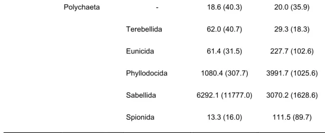
21 Polychaeta - 18.6 (40.3) 20.0 (35.9) Terebellida 62.0 (40.7) 29.3 (18.3) Eunicida 61.4 (31.5) 227.7 (102.6) Phyllodocida 1080.4 (307.7) 3991.7 (1025.6) Sabellida 6292.1 (11777.0) 3070.2 (1628.6) Spionida 13.3 (16.0) 111.5 (89.7)
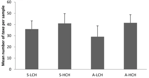
In figure 2, we can see that in terms of mean abundances of individuals, all the groups showed similar abundances, expect for the low complex habitats in autumn, which has lower values of abundances. As for the mean number of species (figure 3), we see that within each season the high complex habitats were associated with a higher number of species than the low complex habitats, particular in autumn.
Figure 2: Mean number of individuals sampled collected through the method of quantitative biomass collection in a quadrate. S-LCH: Summer low complex habitats; S-HCH: Summer high complex habitats; A-LCH: Autumn low complex habitats; A-HCH: Autumn high complex habitats. 0 200 400 600 800 1000 1200 1400 1600 1800 2000 S-LCH S-HCH A-LCH A-HCH N u m b e r o f in d iv id u als p e r sa m p le
22
Figure 3: The mean number of species sampled through the method of quantitative biomass collection in a quadrate. S-LCH: Summer low complex habitats; S-HCH: Summer high complex habitats; A-LCH: Autumn low complex habitats; A-HCH: Autumn high complex habitats.
The PERMANOVA analyses, showed that in the samples collected with the biomass collection method (table 2), there was only a significant interaction between sampling events (nested within season) and location (nested within substratum complexity) (p<0.01).
Table 2: PERMANOVA results showing the differences between the samples collected with the biomass collection method. Significant differences are highlighted in bold. Se- Season; HC-Habitat complexity; Da- data of sampling; Lo-Location of sampling.
Source Degrees of freedom Sum of squares Mean of sum
squares Pseudo-F P(perm)
Unique perms Se 1 4984.5 4984.5 1.2 0.4 9955 HC 1 5037.8 5037.8 2.6 0.1 9957 Da(Se) 1 5491.2 5491.2 3.3 0.1 9949 Lo(HC) 1 943.19 943.2 0.7 0.6 9952 SexSC 1 1990.9 1990.9 1.4 0.3 9939 SexLo(HC) 1 838.9 838.9 0.6 0.7 9938 Da(Se)xHC 1 1804.7 1804.7 1.2 0.4 9937 Da(Se)xLo(HC) 3 4221.8 1407.3 1.7 0.1 9866 Residual 26 21966 844.8 Total 39 51913 0 10 20 30 40 50 60 S-LCH S-HCH A-LCH A-HCH M e an n u m b e r o f ta xa p e r sa m p le
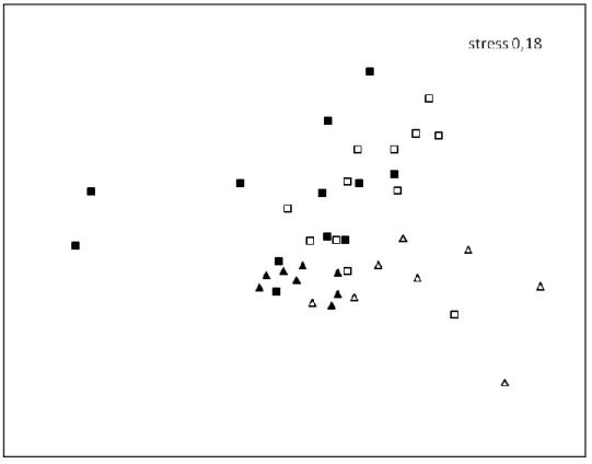
23 The Multidimensional Scaling (MDS) results (figure 4) showed two different patterns. The first tendency pattern was between the two seasons, where it was visible a separation between summer and autumn. The second one consisted in the separation between the low complex habitats from the high complex habitats, more evident inside autumn.
Figure 4: Multidimensional scaling (MDS) depicting ordination of samples, collected through the biomass collection method. Low complex habitats in summer: ; High complex habitats in summer: ; Low complex habitats in autumn: ; High complex habitats in autumn: .
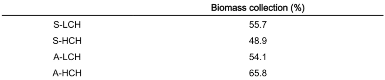
In terms of homogeneity inside the groups of samples (table 3), it showed that the most homogeneous were the high complex habitats in summer and the least homogeneous were the high complex habitats in autumn. When comparing the groups (table 4), the most similar groups were the high complex habitats in summer and autumn, and the most different groups were the low complex habitats in summer and autumn.
24
Table 3: Average similarity in percentage, inside each group of samples (S-LCH: Summer low complex habitats; S-HCH: Summer high complex habitats; A-LCH: Autumn low complex habitats; A-HCH: Autumn high complex habitats), for the method of quantitative biomass collection, calculated trough SIMPER.
Biomass collection (%)
S-LCH 55.7
S-HCH 48.9
A-LCH 54.1
A-HCH 65.8
Table 4: Average dissimilarity in percentage, between the groups of samples (S-LCH: Summer low complex habitats; S-HCH: Summer high complex habitats; A-LCH: Autumn low complex habitats; A-HCH: Autumn high complex habitats), for the method of quantitative biomass collection, calculated trough SIMPER.
Biomass collection (%)
S-LCH S-HCH A-LCH
S-HCH 49.8 - -
A-LCH 50.7 - -
A-HCH - 47.1 48.2
When comparing the habitat complexity within each season (Table 5), all the taxa were more abundant in the high complex habitats than in the low complex habitats. In summer the specie that contributed more for the dissimilarity was the Spirobranchus lamarcki (Quatrefages, 1866). In autumn, the most contributing taxa was the Chthamalidae. In both seasons Polychaeta were the main contributors for the differences between groups.
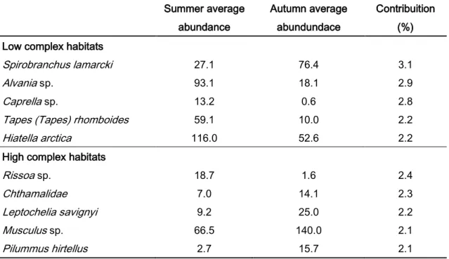
Between seasons within each habitat complexity (table 6), in the low complex habitats all the representative species were more abundant in summer, except Spirobranchus lamarcki, which was more abundant in autumn. Bivalvia and Polychaeta were the main contributors for the difference between groups. In opposition, in the high complex habitats, all the species were more abundant in autumn. The only exception was Rissoa sp., which was more abundant in
25 summer. Bivalvia and Gastropoda were the main contributors to the differences between groups
Table 5: Average abundances per sample of the top five taxa, that contributed more for the differences on the samples between the low complex habitats (LCH) and the high complex habitats (HCH) in summer and autumn, sampled with the biomass collection method.
LCH average abundance HCH average abundance Contribution (%) Summer Spirobranchus lamarcki 27.1 57.4 2.2 Parasinelobus chevreuxi 3.8 14.6 1.8 Gammaridea 5.5 9.6 1.7 Sabellaria alveolata 0.0 7.4 1.7 Sabellaria spinulosa 0.7 7.6 1.7 Autumn Chthamalidae 0.1 14.1 3.2 Nereididae 12.6 84.0 2.8 Sabellaria alveolata 0.4 11.2 2.4 Syllidae 12.7 63.9 2.3 Hiatella arctica 52.6 135.7 2.3
Table 6: Average abundances per sample of the top five taxa that contributed more for the differences on the between seasons in each type of habitat complexity sampled with the biomass collection method.
Summer average abundance Autumn average abundundace Contribuition (%) Low complex habitats
Spirobranchus lamarcki 27.1 76.4 3.1
Alvania sp. 93.1 18.1 2.9
Caprella sp. 13.2 0.6 2.8
Tapes (Tapes) rhomboides 59.1 10.0 2.2
Hiatella arctica 116.0 52.6 2.2
High complex habitats
Rissoa sp. 18.7 1.6 2.4 Chthamalidae 7.0 14.1 2.3 Leptochelia savignyi 9.2 25.0 2.2 Musculus sp. 66.5 140.0 2.1 Pilummus hirtellus 2.7 15.7 2.1 .
26 When the habitat complexity was analysed independently from seasonality (all high complex habitats samples compared with all low complex habitats samples), the high complex habitats showed the higher abundance of taxa (table 7). The only exception was Musculus sp. showing the opposite pattern. The Bivalvia and Polychaeta were the main contributors to the difference between the two groups.
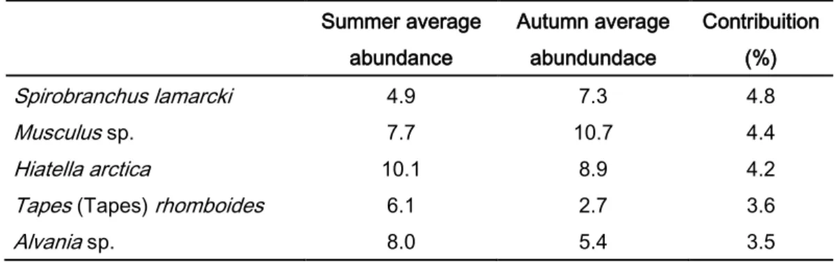
When seasonality was analysed independently from habitats complexity (all summer samples compared with all autumn samples), different patterns were observed (table 8): Spirobranchus lamarcki and Musculus sp. were more abundant in autumn; Hiatella arctica (Linnaeus, 1767), Tapes (tapes) rhomboids (Pennant, 1777) and Alvania sp., were more abundant in summer. The Bivalvia and Polychaeta were the main contributors for the difference between the two groups.
Table 7: Average abundances per sample of the top five taxa that contributed more for the differences between habitat complexities, sampled with the biomass collection method. HCH- High complex habitats; LCH- Low complex habitats.
LCH average abundance HCH average abundance Contribution (%) Spirobranchus lamarcki 5.1 6.7 4.4 Hiatella arctica 8.7 10.5 4.4 Musculus sp. 9.2 8.6 3.9 Nereididae 3.2 6.7 3.6 Alvania sp. 6.8 7.1 3.1
Table 8: Average abundances per sample of the top five taxa that contributed more for the differences between seasonality, sampled with the biomass collection method.
Summer average abundance Autumn average abundundace Contribuition (%) Spirobranchus lamarcki 4.9 7.3 4.8 Musculus sp. 7.7 10.7 4.4 Hiatella arctica 10.1 8.9 4.2
Tapes (Tapes) rhomboides 6.1 2.7 3.6
27 3.2. Intersection points method
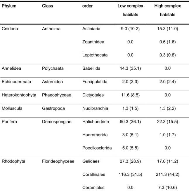
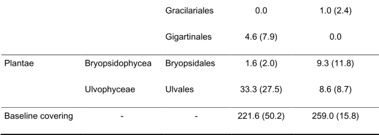
In the intersection point method, there were sampled 3025 individuals and 30 taxa.
The main species present in the low complex habitats were: Demospongiae (Halichondrida), Florideophyceae (Corallinales) and Ulvophyceae (Ulvales). As for high complex habitats, the main species were Demospongiae (Halichondrida) and Florideophyceae (Corallinales) (table 10).
Table 9: The mean abundances (individuals/m2) and its standard deviation, of the taxas sampled by the
intersection point method.
Phylum Class order Low complex
habitats
High complex habitats
Cnidaria Anthozoa Actiniaria 9.0 (10.2) 15.3 (11.0)
Zoanthidea 0.0 0.6 (1.6)
Leptothecata 0.0 0.3 (0.8)
Annelidea Polychaeta Sabellida 14.3 (35.1) 0.0
Echinodermata Asteroidea Forcipulatida 2.0 (3.3) 2.0 (2.4)
Heterokontophyta Phaeophyceae Dictyotales 11.6 (8.5) 0.0
Molluscula Gastropoda Nudibranchia 1.3 (1.5) 1.3 (2.2)
Porifera Demospongiae Halichondrida 60.3 (36.1) 22.3 (15.5)
Hadromerida 3.0 (5.1) 1.0 (1.7) Poecilosclerida 5.0 (5.5) 0.0
Rhodophyta Florideophyceae Gelidaes 27.3 (28.9) 17.0 (11.2)
Corallinales 116.3 (31.5) 211.3 (44.2)
28
Gracilariales 0.0 1.0 (2.4)
Gigartinales 4.6 (7.9) 0.0
Plantae Bryopsidophycea Bryopsidales 1.6 (2.0) 9.3 (11.8)
Ulvophyceae Ulvales 33.3 (27.5) 8.6 (8.7)
Baseline covering - - 221.6 (50.2) 259.0 (15.8)
In terms of mean abundances of individuals (figure 4) and mean number of species (figure 5) there weren’t any apparent differences between seasons or habitat complexity.
Figure 4: The mean abundances of individuals sampled through the method of semi-quantitative intersection points. S-LCH: Summer low complex habitats S-HCH: Summer high complex habitats; A-LCH: Autumn low complex habitats; A-HCH: Autumn high complex habitats. 0 10 20 30 40 50 60 70 80 90 S-LCH S-HCH A-LCH A-HCH M e an ab u n d an ce s o f i n d iv id u asl p e r sam p le
29
Figure 5: The mean number of species sampled through the method of semi-quantitative intersection points. S-LCH: Summer low complex habitat; S-HCH: Summer high complex habitats; A-LCH: Autumn low complex habitats; A-HCH: Autumn high complex habitats.
The PERMANOVA analysis showed that in the samples collected with the intersection points method (table 10), there was a significant interaction between dates within seasons with habitat complexity (p<0.05). Date as a main factor was also significant (p<0.05).
Table 10: PERMANOVA results showing differences between the samples collected with the intersection point method. Significant differences are highlighted in bold. Se- Season; HC-Habitat complexity; Da- Data of sampling; Lo-Location of sampling.
Source Degrees of freedom Sum of squares Mean of sum
squares Pseudo-F P(perm)
Unique perms Se 1 5865.8 5865.8 1.5 0.3 9956 HC 1 3585.1 3585.1 1.9 0.2 9963 Da(Se) 2 7280.6 3640.3 9.2 0.1 9952 Lo(HC) 2 1484.0 742.0 1.9 0.2 9958 SexSC 1 3345.3 3345.3 1.9 0.2 9957 SexLo(HC) 2 1136.0 568.0 1.4 0.3 9934 Da(Se)xHC 2 2737.8 1368.9 3.5 0.1 9963 Da(Se)xLo(HC) 4 1581.3 395.3 0.9 0.6 9915 Residual 32 14047.0 439.0 Total 47 41062.0 0 1 2 3 4 5 6 7 8 S-LCH S-HCH A-LCH A-HCH M e an n u m b e r o f taxa p e r sam p le
30 In the MDS results (figure 6), there was again a tendency pattern separating seasons and habitats complexity, nevertheless the tendency isn’t as obvious as the MDS results for the biomass collection method.
Figure 6: Multidimensional scaling (MDS) depicting ordination of samples collected through the intersection point method. Low complex habitats in summer: ; High complex habitats in summer: ; Low complex habitats in autumn: ;High complex habitats in autumn: .
In terms of homogeneity inside the groups of samples, table 11 showed that the low complex habitats were the least homogeneous and the high complex habitats were the most homogenous, being both in autumn. In terms of similarity between groups, table 12 showed that the high complex habitats in summer and autumn were the most similar in opposite to the low complex habitats in summer and autumn that were the most different.
31
Table 11: Average similarity in percentage, inside each group of samples (S-LCH: Summer low complex habitats; S-HCH: Summer high complex habitats; A-LCH: Autumn low complex habitats; A-HCH: Autumn high complex habitats), for the method of semi-quantitative intersection points calculated trough SIMPER.
Intersection points (%)
S-LCS 61.8
S-HCS 65.8
A-LCS 57.4
A-HCS 68.3
Table 12: Average dissimilarity in percentage, between the groups of samples (S-LCH: Summer low complex habitats; S-HCH: Summer high complex habitats; A-LCH: Autumn low complex habitats; A-HCH: Autumn high complex habitats), for the method of semi-quantitative intersection points calculated trough SIMPER.
Intersection points (%)
S-LCH S-HCH A-LCH
S-HCH 47.9 - -
A-LCH 49.1 - -
A-HCH - 36.1 40.9
When comparing between habitat complexity within each season (table 13), both seasons didn’t showed a clear pattern among the more contributing species. In summer, Corallina elongata (J. Ellis & Solander, 1786) and Anemonia viridis (Forskål, 1775) were more abundant in the high complex habitats, opposite to Ulva lactuca (Linnaeus, 1753), Ciocalypta penicillus (Bowerbank, 1862) and Dictyota dichotoma (J. V. Lamouroux, 1809) that were more abundant in the low complex habitats. In autumn, we had Corallina elongate and Anemonia viridis more abundant in the high complex habitats and Ciocalypta penicillus and Gelidium pusillum (Le Jolis, 1863) more abundant in the low complex habitats.
32 Between seasons within each habitat complexity (table 14), in both types of habitats there wasn’t any evidence of a pattern. In the low complex habitats, Ulva lactuca and Dictyota dichotoma were more abundant in summer, and Ciocalypta penicillus and Gelidium pusillum were more abundant in autumn. As for the high complex habitats, Ciocalypta penicillus and Corallina elongata) were more abundant in autumn and Anemonia viridis, Gelidium pusillum and Ulva lactua were more abundant in summer.
Table 13: Average abundances per sample of the top five taxa that contributed more for the differences between habitat complexity within seasonality, sampled with the intersection points method. HCH- High complex habitats; LCH- Low complex habitats.
LCH average abundance HCH average abundance Contribution (%) Summer Corallina elongata 0.1 4.1 12.7 Ulva lactuca 7.4 2.1 11.4 Ciocalypta penicillus 3.5 0.8 10.4 Dictyota dichotoma 2.1 0.0 9.8 Anemonia viridis 1.0 1.9 8.8 Autumn Corallina elongata 1.3 9.1 14.9 Ciocalypta penicillus 11.2 3.3 13.1 Gelidium pusillum 6.6 1.7 11.9 Anemonia viridis 0.3 1.8 6.9 Baseline covering 19.1 32.1 6.8
33
Table 14: Average abundances per sample of the top five taxa that contributed for the differences between seasonality within the habitat complexity, sampled with the intersection points method.
Summer average abundance Autumn average abundundace Contribuition (%) Low complex habitats
Ulva lactuca 7.4 0.9 11.6
Ciocalypta penicillus 3.5 11.2 10.5
Dictyota dichotoma 2.1 0.1 9.5
Gelidium pusillum 0.0 6.6 9.4
Baseline covering 36.3 19.1 6.6
High complex habitats
Ciocalypta penicillus 0.8 3.3 13.2
Corallina elongata 4.1 9.1 12.3
Anemonia viridis 1.9 1.7 11.2
Gelidium pusillum 2.5 1.8 11.1
Ulva lactuca 2.1 0.1 8.9
When the habitat complexity was analysed independently from seasonality (all high complex habitats samples compared with all low complex habitats samples) (table 16), the Ulva lactua was more abundant in summer and Lithophyllum incrustans (Philippi, 1837), Ciocalypta penicillus and Corallina elongata were more abundant in autumn, resulting on not apparent pattern. Finally, When seasonality was analysed independently from habitats complexity (all summer samples compared with all autumn samples) (table 15), we couldn’t assume a clear pattern, with Lithophyllum incrustans and Corallina elongata being more abundant in the high complex habitats and with Ciocalypta penicillus and Ulva lactuca being more abundant in the low complex habitats.
34
Table 15: Average abundances per sample of the top five taxa that contributed more for the differences between habitats complexity sampled with the intersection points method. HCH- High complex habitats. LCH- Low complex habitats.
LCH average abundance HCH average abundance Contribution (%) Baseline covering 27.7 32.4 19.7 Lithophyllum incrustans 13.9 19.8 18.4 Ciocalypta penicillus 7.3 2.1 12.9 Corallina elongata 0.7 6.6 11.1 Ulva lactuca 4.2 1.1 8.8
Table 16: Average abundances per sample of the top five taxa that contributed more for the differences between seasons with the intersection points method.
Summer average abundance Autumn average abundundace Contribuition (%) Baseline covering 34.5 25.6 20.6 Lithophyllum incrustans 13.8 20.0 18.6 Ciocalypta penicillus 2.2 7.3 13.1 Ulva lactuca 4.8 0.5 9.4 Corallina elongata 2.1 5.2 9.4
35 4. Discussion
The scale dimension originates changes on the structure of the communities (e.g., Turner et al., 1989; Steele, 1991; Thrush, 1991), and differences on sampled species. Such effects were observed in the present study. In general we saw that in the biomass collection method, the main taxa sampled were the Bivalvia, Gastropoda, Malacostraca and Polychaeta. As for the main taxa sampled by the intersection point method, they were Demospongiae, Florideophyceae and Ulvophyceae.
Vagile species were the most abundant group on the quantitative biomass samples, in opposition to the intersection point method, where sessile species were more abundant, confirming previous results (Boaventura et al., 2002; Sconfieti et al., 2003). These different scales sampled is probably related to the different mobility and size of the organisms and with the characteristics of the methodologies. Although the differences obtained at the two scales, these two approaches are complementary, providing different levels of information (Sconfietti et al., 2003; Marchini et al., 2004; Parravici et al., 2009).
A slightly tendency to more homogenous communities was observed in the larger scale trough the sessile organisms, a pattern also observed (Garrabou et al., 1998; Erlandsson et al., 2005), were the algal dominated communities showed the lowest spatial heterogeneity when compared with the invertebrate communities. According to some authors, the larger heterogeneity exhibited by the vagile benthic species results from their r-selected life-history, that consists in a large initial increment of opportunists individuals in order to colonize the environment (Lu & Wu, 1998).
Results from the biomass collection method (dominated by vagile species) seemed to be more sensitive to habitat complexity and seasonality, than the sessile communities evaluated by intersection point method that presented a
36 low level of change across the studied factors. This may be related to seasonal changes of benthonic invertebrates (Silva, 2006), and/or by the effect of scale where bigger scales tend to reduce the resolution (Allen & Hoekstra, 1991; Schneider, 1994; Schneider et al., 1997).
The habitat complexity creates a great variety of different microhabitats and niches, permitting the species to co-exist, contributing to within-habitat diversity (Pianka, 1988), and creating refuge conditions from predators contributing for different abundances between simple a complex habitats (Franchetti et al., 2003). The influence of habitat complexity seems to be more evident in autumn than in summer, where, due the recruitment season, organisms tend to colonize both types of habitats. Again this is a consequence of the opportunistic benthic species r-selected life-history, that causes them to quickly and in large number colonize new niches more efficient that their competitors. Through time, these initial colonizers will be replaced by other species, more able, causing for the populations to become more homogenise as seen in winter (Lu & Wu, 1998).. Life cycles, influencing growth, reproduction, abundance and the species endurance (Coma et al., 2000) can explain this fact.
Townsend et al. (1997) described for the freshwater benthic communities that the high complex habitats tend to be colonized by more specialized species and the homogeneous by more general species. Because of being more adapt, the organisms are allowed to better endure to the seasonal changes and predators, maintained more similar to the summer levels, leading to a less drastic change in the communities of the high complex habitats. The opposite occurs for the species less specialized, which vary more depending on the conditions
The higher abundance of sessile community observed at complex habitats in autumn, also provides additional shelter and protection for the vagile species (Connell, 2003; Wernberg & Connell, 2008) which can explain the higher abundances.
37 Concerning the habitat complexity, the high complex habitats showed to be preferred by Hiatella artica, Alvania sp., Coralina enlogata, Spirobranchus lamarcky, Litophylum incrustans and Neireididae. The principal reason for these preferences were the protection given by these habitat, as seen through literature for Hiatella artica, Alvania sp., Litophylum incrustans (Reidl, 1983), Spirobranchus lamarcky (Chapmand et al., 2007) and Neireididae (Gibson, 2001).
The low complex habitats demonstrated to be more colonised by Ulva lactuca, Musculus sp. and Ciocalypta penicillus. These preference were registered due to their resistant to the hydrodynamic disturbance, given an advantage in relation to other species, as seen for Ulva lactuca (Chapman & Underwood, 1998), Musculus sp., Ciocalypta penicilus (Gibson, 2001) and Coralina enlogata (Wernberg et al., 2008).
In terms of seasonality, in both scales, although the general tendency to separate seasons and habitat complexity within seasons, seasonality seems to be the main driving force to the community. However, habitat complexity seems to be important to community structure when associated with seasonal effect. The observed less importance of habitat complexity in the community structures, in opposition to other studies (McCormick 1994; Kostylev 1996; Petren & Case 1998), may result from the temporal proximity of the samples, lower than 3 months, as well as from the existence of different habitats on the surroundings enabling the migration between different zones by the species and causing the migration of none characteristic species (Pacheco, 2010). Because of the bad conditions register in the winter, and because of the lack of laboratory time, in autumn it was only possible to analyse 4 of the 6 replicates in each habitat, which may have caused some interference in data.
According to Pacheco (2010), during early colonization, high variability is generated as well as high abundances, and gradually these effects diminish as
38 succession proceeds. This tendency is also observed by Antoniadou et al. (2011) that observed a faster colonization period during winter by the communities, because of the lower biological interactions and species densities, as observed to intertidal zones (Chapman & Underwood; 1998; Foster et al., 2003).
Such dynamic was also described in Ballesteros developed phase (1991, 1992) which says that the dominant species reach the maximum coverage values corresponds to the lowest spatial heterogeneity. In contrast, the diversified phase occurs when dominant species reached minimum coverage values, and corresponds with the maximum heterogeneity in spatial pattern. This can be the reason for the most homogenous communities being in autumn, especially in the high complex habitats, when the diversity is lower, as showed in the results. Opposite the results showed that the groups more heterogenic and similar were the groups in summer, probably due to the large dispersion and expansion of the benthic recruitment.
Several taxa were the main responsible for the seasonal differences. Taxa with stronger association with summer were Hiatella artica, Alvania sp., Tapes rhomboids and Ulva lactuca. These species show preference for the summer mainly because of the settlement season being at this time, for exempla, Hiatella artica and Tapes rhomboids (Morvan & Ansell, 1988; Sejr et al., 2002) and because of the favourable conditions in this season, for exempla Ulva lactuca (Chapman & Underwood, 1998). The taxa more associated to autumn were Spirobranchus lamarckii, Musculus sp., Ciocalypta penicillus, Litophylum incrustans and Coralina enlogata. These happened probably because of some species spawning naturally closer to autumn like Spirobranchus lamarckii (Chapmand et al., 2007).
In summary, has it would be expected, there were some significant different distributions among the species depending on the habitat complexity and the
39 seasonality (Johnson et al., 2003; Antoniadou et al., 2011), however the patterns that resulted from the comparison between habitats weren’t as obvious as expected and the seasonality alone appeared to be a bigger main driven factor.
From this study we can conclude: a) the method of quantitative biomass and the method of semi-quantitative intersection points are complementary and not similar, b) There are clearly species that characterise different seasons and habitats of different complexity, c) and that the pattern between high and low complex habitats as well as seasonally could be more evident with the improvement of the experimental approach, but overall the biomass collection method seemed to be the most appropriated. The hypothesis of higher richness and abundances be associated to higher complex habitats was partially confirmed. In fact, this tendency was observed but not inducing significant differences as important as seasonality.
For future studies on this theme, the replicates should be more separated temporally, being the seasonal pattern quantified at the beginning and end of each season (separation of 1 to 3 months), and taking place in larger homogenous areas, avoiding the migration between different zones by the species (Pacheco, 2010).
Also, the efficiency of the quantitative biomass collection in a quadrate could be enlarged by introducing an air-lift (suction sampler) to prevent the escape of the mobile fauna (Bianchi et al., 2004).
40 References
Allen, T. F. H., Hoekstra, T. W., 1991. Role of heterogeneity in scaling of ecological systems under analysis. In: Ecological Heterogeneity, Kolasa, J., Pickett, S.T.A. (eds.), Springer-Verlag, pp: 47–68.
Anderson, M. J., Gorley, R. N., Clarke, K. R., 2008. PERMANOVA+ for PRIMER: guide to software and statistical methods. PRIMER-E Ltd, Plymouth. U.K.
Antoniadou, C., Voultsiadou, E., Chintiroglou, C., 2011. Seasonal patterns of colonization and early succession on sublittoral rocky cliffs. J. Exp. Mar. Biol. Ecol., 403(1-2): 21-30.
Ballesteros, E., 1991. Structure and dynamics of north-western Mediterranean phytobenthic communities: a conceptual model. Homage to margalef; or, why there is such pleasure in studying nature (Roas, J. D. & Prat, N., eds) Oecol. Aquat., 10: 223-242.
Ballesteros, E., 1992. Els vegetals I la zonación litoral: espécies, comunitats i factores que influeixen la seva distribuiciò. Arxius de la secciò de Ciències CI Institut d’Etudis Catalans, Barcelona, España.
Bianchi, C. N., Pronzato, R., Cattaneo-Vietti, R., Benedetti Cecchi, L., Morri, C., Pansini, M., Chemello, R., Milazzo, M., Fraschetti, S., Terlizzi, A., Peirano, A., Salvati, E., Benzoni, F., Calcinai, B., Cerrano, C., Bavestrello, G., 2004. Hard bottoms. Biologia Marina Mediterranea, 11: 185-215.
Bilyard, G.R., 1987. The value of benthic infauna in marine pollution monitoring studies. Mar. Pollut. Bull., 18: 581-585.