Predicting Chelonia mydas nests survivability
rates with use of Machine Learning techniques
Applying Machine Learning techniques on
conservation data – case study
David Tiago Calçada
Dissertation submitted in partial fulfillment of the
requirements for the degree of master’s in information
management
NOVA Information Management School
Instituto Superior de Estatística e Gestão de Informação
Universidade Nova de LisboaPredicting Chelonia mydas nests survivability rates with use of
Machine Learning techniques
Applying Machine Learning techniques on conservation data – case study
David Tiago Calçada
Dissertation presented as the partial requirement for obtaining a Master's degree in Information Management, Specialization in Knowledge Management and Business Intelligence
Advisor: Mauro Castelli Co-supervisor: Illya Bakurov
Acknowledgements
I simply cannot thank the Príncipe Foundation enough for allowing me to work on such a project. Special thanks to Estrela Matilde, Vanessa Schmidt and Frazer Sinclair for their time and contribution to this thesis. I wish them continuous success and that we might continue to collaborate in conservation biology studies in the near future.
To my coordinators Professor Illya Bakurov and Professor Mauro Castelli, you have my eternal gratitude for your patience and support. Your guidance was more than enlightening.
To my family who kept pushing me to go beyond what I believed were my limitations and to my friends who kept me motivated throughout. You have my love and appreciation.
I would like to make a special dedication to my grandfather who taught me to never give up, no matter what obstacles get thrown in your way.
Abstract
It is the generalized goal of knowledge discovery techniques to help us find useful patterns in data whilst not subjecting us to the ambiguity and overcomplexity of models. In fact, it has become increasingly important to allow for a common language to exist between biologists and data scientists.
In my thesis I aim to make use of Green Turtle (Chelonya mydas) nesting data obtained in surveys conducted from 2015 to 2019 in Príncipe Island, in order to obtain two things: Firstly, to understand insights related to sea turtle survivability rates; Secondly, to develop prediction models on said rates via popular Machine Learning algorithms. For this purpose, I will detail how my collaboration with the sea turtle conservation team in Principe Island began, and work has been developed since.
I will describe all steps referring to the dataset transformation, manipulation and exploration, and detail how each step has allowed me to feed the sea turtle data into powerful Machine Learning algorithms that are to be evaluated against their ability to predict accurate nest survivability rates.
At the end of the contextual part of this document, I will explain my findings and present the limitations of this project; I hope to provide a solid example that will allow future students and researchers to keep in mind what challenges await them should they pursue this field.
Finally, a key aspect of this thesis that is very important that it’s written in such a way that individuals with different backgrounds are able to understand its content and objectives. Keywords: knowledge discovery, green turtle, dataset transformation, manipulation and exploration, Machine Learning algorithms;
INDEX
1. Introduction ... 1
1.1 Context and importance ... 1
1.2 Current research ... 1
1.3 My contribution... 1
1.4 Structure ... 2
1.5 Tools ... 2
2. Theoretical revision ... 3
2.1 São Tomé and Príncipe ... 3
2.2 Turtle species in Príncipe... 5
2.3 Previous studies on the area ... 7
2.3.1 Research on species survival ... 7
2.3.2 Prediction ... 9
2.3.3 Machine Learning in biological data ... 9
2.3.4 Pooled data ... 10
2.3.5 Machine Learning algorithm selection ... 11
2.4 Machine Learning Algorithms and benchmark creation ... 12
2.4.1 Benchmarking ... 12
2.4.2 Supervised learning ... 12
3. Príncipe Foundation (PF) and analysis focus points ... 19
3.1 The organisation ... 19
3.2 The cases ... 19
3.3 Data collection and presentation ... 20
4. Data Pre-processing ... 21
4.1 Data set transformation ... 21
4.2 Variable set ... 23 4.2 Exploration ... 26 4.2.1 Outlier removal ... 26 4.2.2 Correlation matrix ... 28 4.3 Feature extraction ... 29 4.4 Feature selection ... 29 4.4.1 Linear regression ... 29
4.3.2 Recursive feature selection with cross validation (RFSCV) ... 32
4.3.3 Boruta package ... 33
4.3.4 Random Forest variable importance ... 34
4.3.4 Subset variable assessment... 36
5.1 Benchmark ... 45
5.1.1 Artificial Neural Network ... 46
5.1.2 Bagging or bootstrap aggregation ... 46
5.1.3 Random Forest ... 46
5.1.4 Adaptive boosting ... 46
5.1.5 Gradient boosting ... 47
5.1.6 Xgboost ... 47
5.2 Evaluation of results ... 48
5.2.1 Mean Absolute Error (MAE) ... 48
5.2.2 Mean Squared Error (MSE)... 48
5.3 Results ... 49
6. Conclusion ... 50
7. Final remarks ... 51
7.1 PF cases assessment (limitations) ... 51
7.1.1 Prediction of STNSR ... 51 7.1.2 Dataset ... 51 7.1.3 Mapping ... 51 7.2 Conclusive paragraph ... 52 8. REFERENCES ... 53 9. ANNEXES ... 56
ANNEX I - Fundação Príncipe organization information ... 57
ANNEX II – Species description ... 58
II.I - Chelonia mydas (CM) ... 58
II.II - Eretmochelys imbricata (EI) ... 59
II.III - Dermochelys coriacea (DC)... 60
ANNEX III – Data sets description ... 61
III.III – Coordinates ... 64
III.IV weather_stp ... 64
III.IV - weather_stp ... 65
ANNEX IV – Model of data manipulation phase ... 66
ANNEX V – Correlation map ... 68
ANNEX VI - Feature extraction methods applied in the context of this thesis ... 69
VI.I Principal Component Analysis (PCA) ... 69
VI.II Support Vector Machine (SVD) ... 70
FIGURE INDEX
Figure 1 representation of Príncipe island with 2 submaps ... 4
Figure 2 pie chart on the percentage of nests belonging to each species ... 5
Figure 3 bar plot for trend ... 10
Figure 4 an example of a CM nest digged open for analysis. ... 20
Figure 5 Summary framework for dataset transformation ... 22
Figure 6 summary plot for outlier removal ... 26
Figure 7 correlation heatmap ... 28
Figure 8 plot for recursive feature selection ... 32
Figure 9 plot for relative variable importance ... 34
Figure 10 histogram for anomalies ... 36
Figure 11 pie chart for nests with abnormalities ... 37
Figure 12 histogram for eggs with yolk ... 38
Figure 13 histogram for eggs with embryo ... 38
Figure 14 scatter plot for precipitation ... 40
Figure 15 bar and scatter plot for temperature levels per month ... 41
Figure 16 scatter plot for precipitation levels per month ... 41
Figure17 bar plot for survival rate per month ... 42
Figure 18 scatter plot for nest depth ... 43
Figure 19 scatter plot for nest length ... 44
Figure 20 PF logo ... 57
Figure 21 CM adult turtle. ... 58
Figure 22 CM younglings. ... 58
Figure 23 EI adult turtle. ... 59
Figure 24 EI younglings. ... 59
Figure 25 DC adult turtle. ... 60
Figure 26 DC younglings. ... 60
Figure 27 data maniputation summary ... 68
Figure 28 correlation matrix with values ... 68
Figure 29 PCA elbow graph ... 69
Figure 30 summary graph ... 70
TABLE INDEX
Table 1 summary for nest counts and percentage for all beaches ... 6
Table 2 summary table for artificial neural network strengths and weaknesses ... 13
Table 3 summary table for bagging strengths and weaknesses ... 14
Table 4 summary table for random forest strengths and weaknesses ... 15
Table 5 summary table for adaptive boosting strengths and weaknesses ... 16
Table 6 summary table for gradient boosting strengths and weaknesses ... 17
Table 7 summary table for Xgboost strengths and weaknesses ... 18
Table 8 referring to egg status ... 23
Table 9 referring to nest status ... 23
Table 10 referring to turtle anatomy ... 23
Table 11 referring to nest predation ... 23
Table 12 referring to geographical and climate factors ... 24
Table 13 referring to date and time ... 24
Table 14 referring to other variables ... 24
Tabela 15 calculation of mortality and survivability ... 24
Table 16 summary for heteroscedasticity test ... 30
Table 17 summary for OLS r-squared ... 30
Table 18 boruta parameter tuning ... 33
Table 19 boruta random forest tuning ... 34
Table 20 summary for egg status ... 39
Table 21 table summary on egg size ... 43
Table 22 parameter tunning for ANN... 46
Table 23 parameter tunning for bagging ... 46
Table 24 parameter tunning for Random Forest ... 46
Table 25 parameter tunning for Adaptive boosting ... 46
Table 26 parameter tunning for Gboost ... 47
Table 27 parameter tunning for Xgboost ... 47
Table 28 summary results for MAE ... 48
Table 29 summary results for MSE ... 48
Table 30 PF contact information ... 57
Table 31 summary on CM ... 58
Table 32 summary on EI ... 59
Table 33 summary on DC ... 60
Table 34 master file A.Seguimento actividade fêmeas ... 61
Table 35 masterfile B.Seguimento de ninhos... 62
Table 36 Eclosões file ... 63
Table 37 coordinates file ... 64
Table 38 weather summary file ... 64
1. Introduction
1.1 Context and importance
Ethology, the study of animal behaviour has been the focus of countless research studies carried out by both biologists and data scientists. By looking into animal data, we can attempt to learn and understand more about the reasons behind several natural phenomena and in turn, exercise human action when it comes to improving species abundance and welfare. This is where I believe I can make a contribution to conservation biology.
For such a thing to happen, it is crucial to work closely with conservation professionals in order to not only obtain the biological data, but to also acquire meaningful insights about the species and their behaviour. This constitutes the key approach to this thesis.
At this point I would like to introduce the Príncipe Foundation (PF) (ANNEX I), a non- governmental organisation (NGO) with the goal of protecting wildlife in Príncipe Island, including of course, the sea turtles. With their help, I have been able to obtain a dataset containing variables that include sea turtle nesting behaviours and sea turtle anatomical and biological description.
To validate the research and its title, I have, together with the conservation team and my academic coordinators, established the contents of this document. It falls under an umbrella that is best described as applying predictive algorithms in order to obtain sea turtle nest survivability rates (STNSR). Before this, I will demonstrate a thorough analysis on the data providing a step by step view of what I have learned.
1.2 Current research
After gaining a better understating of the context of the topic at hand, it would be pertinent to mention where current studies are lacking or have failed to meet expectations.
Through the years, many studies have focused on animal species with the aim of answering a specific question, be it through knowledge discovery or exemplification of an established hypothesis. Yet, there are considerably few studies that marry standard exploratory approaches on animal data with the powerful predictive capability of Machine Learning algorithms while maintaining a simple and organized structure on both sides.
In fact, it seems that in current times the goals of biological studies appear to be about procuring a balance between how much data understanding we can achieve versus keeping it grounded on a strong theoretical basis. Several studies have been built on this principle, and I will look to further explore some examples in subchapter 2.3.
1.3 My contribution
Referring to the above subtitle, my purpose is to combine an exploratory analysis on sea turtle data with the predictive capabilities of Machine Learning (ML) algorithms to achieve sea turtle nest survivability rates with feasible results.
Specifically, I aim to not only provide useful insights on sea turtle nesting status, but to also provide a basic framework from which future analytical projects can derive from (be it for the same topic or not). To achieve this, I have attempted to provide my findings in the clearest way possible while avoiding the ambiguity and abstraction that regression analysis typically leads us to.
1.4 Structure
To conclude my introduction to this thesis I will refer to the structure I will follow throughout: In chapter 2, I present the theoretical background from which my research extends from. In the first subchapter, a short description of the country of São Tomé and Príncipe will be given with a focus on social, economic, meteorological and geographical contexts.
The next subchapter includes references to documents that approach conservation topics in Príncipe Island. I will be looking to discuss what approaches were used and what was discovered. I intend to explore possible limitations and where further developments could be made. To contextualize ourselves in the regression problem that we are dealing with, the next titles will introduce concepts of Time series and Prediction and how these are relevant in the greater context.
To shore up this chapter, I will introduce Machine Learning algorithms and their use today. This includes a presentation of the algorithms I will be using in my thesis and the reason they were selected.
Chapter 3 will proceed with a description of the PF and their work on sea turtle conservation in Príncipe Island. I will describe the details of our collaboration and how together we established what topics I would focus my analysis on.
Chapter 4 will be divided between the pre-processing of the data and my exploratory approach to it. It will include the framework summary of what changes were needed for the data in order to have it in a structured form, as well as the establishment of the research cases that the NGO has asked to me to focus on.
Chapter 5 will then make use of the structured and clean data that was achieved previously and apply it to a benchmark with tuned parameters for the algorithms that were explained in Chapter 2. A presentation of the results and their meaning will follow.
Subsequently, in chapter 6 I will discuss the results and approaches accomplished thus far. I will present my overview over the whole document but focusing on the key learning aspects that were achieved. My assessment will focus not only on each step of the analysis, but on the big picture, allowing me to comment on the progress against my goals.
Finally, chapter 7 will contain both the discussion with my final remarks on the work done with limitations being presented in the context of what was set out to accomplish, as well as my response to the cases that the PF asked me to focus on, with recommended guidelines for the future and where to correct possible mistakes.
1.5 Tools
For the purpose of this thesis, I have made use of the Python programming language. After sourcing the excel files containing the turtle data, I have worked on the Anaconda distribution version 3 with Spyder1 platform (4.0) to develop the coding steps for my analysis as well as to
run my algorithms.
I have built my visual aids on Plotly and Seaborn Python libraries.
2. Theoretical revision
2.1 São Tomé and Príncipe
The islands of São Tomé and Príncipe are the two main islands that constitute the archipelagos of the Democratic Republic of São Tomé and Príncipe, an African country located of the western continental coast in the Gulf of Guinea [2, 14].
History
They were uninhabited until a Portuguese arrival on the 15th century gradually started colonizing the island and turning it into a commercial trade station. It remained under Portuguese authority until it obtained its independence in 1975, attaining a democratised form of government. Its culture is based on both African and European influences, as it can be seen in the country’s customs and music.
Political, economic and social
Currently São Tomé and Principe is the second smallest sovereign nation in Africa with a 2018 study estimating around 201,800 individuals constituting its population, harbouring a mix of African natives and mestizo descent.
Economically the country harbours a high dependence on the exportation of cocoa (representing 95% of all agriculture exports), with a reasonably small fishing sector followed by an even smaller industrial sector. The countries government has nonetheless attempted to integrate tourism as an economical sector, but high restriction on nature conservation and subpar logistics have made this undertaking arduous. Also noticeable is the country’s parallel economy that up until more recent times was heavily based on poaching for several native birds, land animals and sea species (including sea turtles).
Geography and climate
São Tomé is 50 km (30 mi) long and 30 km (20 mi) wide and the more mountainous of the two islands.
In comparison, Príncipe is about 30 km (19 mi) long and 6 km (4 mi) wide, making it the smallest of the two.
The climate is tropical with rain occurring mostly during October to May. High temperatures are at sea level, while there are more mild temperatures as one treads inland and into higher altitude grounds.
Due to the Príncipe’s volcanic constitution, its soil is rich in sustenance for plants, which led to a prominent domestic plantation agriculture that is mainly used for exportation. Its land area is mostly covered with rich and varied flora that retains large amounts of its endemic background, although this has suffered significant changes due the transformation of the islands ground into plantation fields.
Beaches
Given we will be only looking into the beaches where a certain sea turtle species make their nests, the focus will be on detailing the geographical data of those same ones. All the 8 beaches that can be found on the dataset can be described as small white sand beaches with the tropical forest line a few meters from the tide line. A map showing the overall geography of Príncipe is given below, where markers pinpoint the location of the beaches we will be looking at:
Figure 1 representation of Príncipe Island with 2 submaps
At the bottom we have INFANTE and BUMBO, on the top right corner box we have MICOTO, RIBEIRA IZÉ and BOMBOM with GRANDE, MACACO and BOI shown on the middle box at the right
Human activity
As we can see on the above figure, there is human presence in the island with Santo António being the main hub of the island served with an airport and harbour that allows for travel between the two islands and to mainland Africa. There is a designated protected area that aims to limit human activity at important natural landmarks. The line that establishes the frontier of this park is seen with the green light that crosses the middle of the island. Important to notice as well is that most beaches are located outside the natural park area, showing that the delimitation of the natural park area was not particularly driven by the sea turtle conservation effort. For this purpose, several volunteers conduct patrols on the several beaches, with the aim of preventing poaching of nesting turtles and their nests.
2.2 Turtle species in Príncipe
As the title suggests, we are only looking to study one species of sea turtle and their nests in the island of Príncipe, as one PF have concentrated their conservation efforts on, and the sites where the data was collected. That said, I can introduce the 3 turtle species the NGO focuses most of its analytical and conservation work: Green turtle (Chelonia mydas) (ANNEX II.I), Leatherback turtle (Dermochelys coriacea) (ANNEX II.III) and Hawksbill turtle (Eretmochelys imbricata) (ANNEX II.II).
The Green turtle (Chelonia mydas)
The Chelonia mydas (CM) is known as green turtle due to the characteristic greenish hue on the back and the colouring of its flesh. It measures on average about 83-114 cm long, weighing anywhere between 110-190 kg. It is not the biggest sea turtle species nesting in Príncipe2, or the
one that lays the most eggs. The interesting aspect of this species is that it is by far the most numerous, as being attracted to tropical climates has made the CM a frequent visitor to the beaches of Príncipe and one of the PF’s main contributors to turtle data collection. This resulted in a more complete set of data on this species and its behaviour in the island. From the pie chart below we can see the percentage on the total number of nests for 3 turtle species:
Figure 2 pie chart on the percentage of nests belonging to each species
Supported by what we can see in figure 2, the decision to focus on CM data comes mostly from the cheer dominance on the volume of data that relates to this species, and due to the fact that it is not possible to assess the other 2 species at this time due to highly incomplete data in the source files.
2 The DC is quite larger, yet significantly less frequent sightings of them at the beaches of Príncipe have left data gathering in a complicated state.
Nesting
The CM has its nesting season in intervals of two years; after mating, the female will approach the beach and use its back flippers to dig a nesting chamber that can on average measure 22-54 centimetres (8 – 21 inches) deep. It will then lay within a range of100 to 126 eggs and proceed to cover the nest with sand, again by making use of its back flippers before getting back to sea. These eggs will then take up to 60 days to incubate inside the nest.
To give an idea of the nesting frequency and presence of this species in Príncipe, there have been over 3003 CM nests in 2019 alone. The team has assured me, along with a quick analysis
on the data, that the same turtle can nest several times per season. So even when looking at the grand total of nests made during the period of 4 years that is assessed, we must take the latter fact to consideration.
Looking at the data from the last 4 calendar years, it becomes increasingly obvious that the CM are the most numerous and frequent nesters. Even considering the 2-year interval between nesting seasons, a CM can nest several times during this period, with an average of 3-5 nests per season [17]. The reason one must insist in mentioning the existence of different nests being made by the same turtle is to clarify that each nest will be considered independent of each other, meaning I will not consider at this stage that each nest formation is dependent on the previous one.
Understanding what beaches the CM tends to nest on more often comes next. Beach count and percentage
Beach name Count Percentage
GRANDE 644 82,04% INFANTE 97 12,36% BOI 34 4,33% BOMBOM 3 0,38% RIBEIRAIZE 2 0,25% MICOTO 2 0,25% BUMBO 2 0,25% MACACO 1 0,13%
Table 1 summary for nest counts and percentage for all beaches
As is it noticeable in table 1, out of 8064 nests, the vast majority of them are lain in the beach of
Grande. Through Príncipe Foundation’s feedback, it is understandable that this is indeed the most widely used beach by the CM due to its size and location. Although we can see that there is only one nest in the beach of Macaco, we must take into account that the dataset that is used will only keep rows with complete information on each individual nest. Although we can assume there are more nests on that particular beach, we just do not have the data to properly verify it. This means that if it came to be that the beach where the nest is made is pertinent for STNSR, a careful but limited assessment must be made.
3 This number accounts for the number of rows on the 2018/2019 nesting season. 4
2.3 Previous studies on the area
2.3.1 Research on species survival
Typically, the classic approach to this research topic has been made via using classical models that test hypothesis based on new or past existing theories constructed on grounded literary work. Unfortunately, this approach rarely allows for the implementation of more interesting pattern discovery techniques that might create the foundations for new ideas altogether. Having said that, current research papers tend to approach the topic of animal behavioural analysis in a fashion similar to what is being done in this thesis. Two recent studies conducted in Príncipe were a good basis to understand what type of approach one needs to take in order to further expand this ideology.
Rapid decline of the endemic giant land snail Archachatina bicarinata on the island of Príncipe, Gulf of Guinea by Dallimerand M. and Melo M. [10]:
The first example is a paper made on the population decline of the endemic Giant Land Snail. It goes through the effort of identifying key human factors that lead to fewer individuals of this species existing in the island of São Tomé by applying surveying actions through the island’s different geographical landscape and then conduction analysis on the results.
Due to the purpose of this paper, there isn’t much exploration on advanced methods for knowledge discovery, but instead a bigger focus on establishing a basis for good explanatory variables. The writers claim:
“We used multiple regression, with both the abundance of live snails (snailabundance) and the occurrence of live or dead individuals (snail presence) as the response variables, and measures of habitat type, productivity and location as explanatory variables.”
Keeping in mind that survey and surveillance effort was conducted by these same individuals, it would have been a very time-consuming undertaking to then conduct extensive knowledge discovery using more complex methods than linear regression. Yet, it is indeed pertinent to consider how the use of different feature selection techniques or application of advanced predictive algorithms such as the ones in Machine Learning (ML) literature might have improved on model accuracy for the Giant Snail presence.
Modelling the distribution of São Tomé bird species: Ecological determinants and conservation prioritization THESIS by Filipe Soares [33]:
Filipa looks into endemic vs non-endemic bird species in the island of São Tomé and makes an interesting case for the use of classical regression techniques as she sets out to discover interesting patterns in data that are visually detectable with the use of maps and clustering techniques. With this methodology, it is possible to identify several dozens of different bird species and serves as a good stepping point to what I wished to achieve with my research. In this case, an understanding approach to undiscovered or unsuspecting causes that lead to STNSR.
This thesis conducts a very complete view on data with a very detailed approach to variable importance both relative to natural habitats, as well as the human threat factor. Indeed, it is a good basis to any study on groups of animals of one or several species and a first of its kind in São Tomé and Príncipe.
The methodology is based on:
the calculation of Relative Variable importance in order to identify behavioural differences between different bird guilds;
applying multi linear regression on data;
conducting logistical regression in order to analyse the response of each species to continuous variables, followed by ranking of the relative importance of those said variables;
Again, it would be possible to extend this research further on by advancing it to ML techniques. Having said that, it is understandable that such an endeavour is neglectable for the overall purpose of the thesis and the great results it achieved.
Estimating carrying capacity at the green turtle nesting beach of the East island French Frigate by Shoals G. H. S. Tiwari, M. Baladz, [36]
This paper is also based on a prediction effort made on top of a green turtle nesting habits dataset. In this specific case the author aims to discover if enough nests are being made (carrying capacity) at the different beaches of the archipelagos of East Island Frigate Shoals and understand the causes that might lead to a positive or negative answer. Available to the author is a dataset that contains data from 37 nesting seasons made by green sea turtles in 10 different islands.
For this intent, and much like my thesis, the data is based on a surveying effort and is to be ran through a model that is robust in face of time series data so as to help establish factors that lead to the estimation of the carrying capacity.
Throughout the paper, the author details what are the impacts of factors and if they can be considered important or neglectable for the carrying capacity whilst establishing the framework for the calculation of important variables. Time series analysis is conducted in order to understand the existence of a trend that has led to more or less nests being formed. This is an important consideration especially given the vast time period that the study covers.
In the end it was not only concluded that there is no predominant trend, but also that nesting was carried out mainly in one beach, while the others are considered to be below their carrying capacity. Very important considerations are made for the quality of the data in the surveys and how more information on both geography and climate can help improve the analysis.
I find this paper particularly interesting as it helped me understand what issues tend to arise when analysing historical data based on surveys. It also makes an interesting case for the possibility of added value on one’s analysis by adding more variables that relate to different themes that (in theory) might affect sea turtle nesting habits.
2.3.2 Prediction
In statistics, Prediction is a statement for a future event for a whole population based on the knowledge of a sample of the population.
Objectively, in this research topic it is not enough to have an interesting dataset, it is perhaps even more important to be supported by a team of conservationists with a great understanding of how the data was collected and its meaning. To make full use of this potential, it is wise to attempt to go beyond the application of standard5 regression analysis on prediction and to
explore the output of more developed algorithms.
The use of ML techniques in prediction has existed for many decades in the form of models of many types and purposes. We have continued to extend the boundaries on the work of ML algorithms in attempts to acquire better predictions that seek to beat standard models e.g. linear or logistical regression. The goal is to apply exhaustive search for patterns inside the data that may lead to more accurate results, while operating on higher volumes of data at higher speeds without having to recur to overcomplex specifications of data.
2.3.3 Machine Learning in biological data
When one searches for examples on the use of ML in the area of biology, it is quite common to come across several examples of its use in health [41]. Its contribution to it is undeniable and it seems it will continue to expand into a wider range of fields. Just to give a few examples:
Atomwise: Builds 3D modules out of molecules through a powerful algorithm; DeppVariant: A statement on the use of Deep Learning for genome studies; Cell Profiller: Being able to identify thousands of features in cell groups;
When it comes to health, it is possible to understand that most advancements derive from the need to understanding and visualizing several aspects of an individual’s health. This in turn allows us to develop powerful algorithms that provide accurate results and higher speeds in order to help doctors evaluate someone’s status whilst greatly reducing room for error.
It is regrettably noticeable however, how lacking we are in terms of applying these techniques on other animal species. A recent study article on animal species classification using Machine Learning techniques gives us the following abstract:
“created by collecting the features of ears and eyes from 10 animals and an experiment was
conducted using Machine Learning techniques such as SVM and MLP to classify them as predators or pets.”
This has been the most frequent example nowadays of how we can use ML techniques in order to understand the animal kingdom and create useful tools that helps us identify species in a quick and feasible manner. It seems as though we are lacking vison on the possibility of applying new solutions to old problems, e.g specie survivability prediction or behavioural pattern analysis.
So, in this thesis I will attempt to show that even though I am using ML for a classical regression problem, its use and relevance today are not in any way diminished and I hope to show that learning from such endeavours as these ones will keep pushing us to strengthen and diversify ML to other biological areas.
2.3.4 Pooled data
I am using data collected from 2015 to 2019. In detail, I have nesting data for each season starting from February 2015 to July 2019: The different series are detailed as:
Censo temporada reprodutiva 2015-2016 Censo temporada reprodutiva 2016-2017 Censo temporada reprodutiva 2017-2018 Censo temporada reprodutiva 2018-2019
Having such a structure of data split in different periods, means we are dealing with Time Series [38]. In other words, we have a set of observations on the values that a variable takes at different times.
Yet it is also true that we are analysing a nest and its characteristics when registered at a single point in time, meaning that although a turtle might have nested in 2016 and then came back 2 years later to nest again, these are considered independent happenings from one another and as such show that the data is partly cross-sectional.
The conclusion is that the whole data set can be considered a combination of both Time Series and Cross-sectional, which in this case is named Pooled data.
Figure 3 line plot for trend
When dealing with this type of data, it is important to assess if our target variable has any peculiar trends that can induce seasonality6. If this phenomenon is observed, certain techniques
can be used to fix it and reduce the impact that it may have on statistical analysis.
I can inform that we do not need to worry about this, although in the graph of picture 3 there is drop right at the end of the series, it is taking an STNSR average of only 3 observations out of the 806 total. This, along a quick assessment for trend analysis, showed that I had not any variation that might lead me to believe we are dealing with seasonality. Thus, I do not consider it necessary to apply trend harmonization techniques.
2.3.5 Machine Learning algorithm selection
As I have articulated several times above, I will use popular Machine Learning algorithms to achieve STNSR. Before I state the reasons for my selection, I consider that it is important to introduce the main fields we can categorize them in.
Deep Learning
It’s a subfield of Machine Learning that refers to the algorithms based on the functioning of human cells that we call Artificial neural networks. Studies [5,31] have given a good explanation on why the use of Neural networks has taken centre stage. High volumes of data and higher performance being the most accepted ones. For the purpose of testing how an ANN performed in comparison with the other models, I have decided to insert it in my study.
Ensemble methods
In a broad term, it is a concept that states that combining a set of weak learners can create a stronger one (by decreasing its variance) [27]. In short, what we are doing is using several learning algorithms that can provide us with better prediction power whilst creating a robust model that is strong in terms or variability and resistance to outliers.
The form that these specific methods assume are that of several Decision Trees that can be provided with voting criteria that help them learn how to form the best tree structure. This is achieved by sampling and splitting the data at different points in hope of achieving the lowest possible error deviation from the actual value we are trying to predict.
Going into more detail, we can differentiate the structures of algorithms that fall in this main category as either baggers (bagging type algorithms) or boosters (boosting type algorithms). Given the high amount of documentation that supports the use of these methods in most generalised regression problems, I have decided to use a combination of different algorithms that relay on either boosting or bagging.
Xgboost
Although also an ensemble method based on boosting, it is important to specify why I have selected this algorithm.
For the last 5 years, its popularity has increased as its performance has been documented to have improved drastically, ever since its stable version in 2019. There will be a more theoretical review on Xgboost in the following chapter, but I wanted to clarify that its integration in this research is because I believe that based on its recent popularity, it can outperform all other algorithms [34].
2.4 Machine Learning Algorithms and benchmark creation
2.4.1 Benchmarking
Predicting the STNSR rates will be achieved by using a selected set of Machine Learning algorithms that will be tuned based on a search for the most suitable parameters. This is called a benchmark. An iterative process that selects the best set of parameters for each algorithm based on an evaluation metric. The selection of what parameters the benchmark will build on and how it will evaluate its performance is based on my theoretical study on the area, supported by my understanding on the problem of prediction at hand.
Having said that, it is pertinent to refer to the algorithms7 that are used and to give a brief
explanation on how they fall on the Machine Learning scope as well as their workings based on their literature.
2.4.2 Supervised learning
Unlike unsupervised learning where we are unaware of patterns in data and make no use of pre- existing labels, here not only do we have historical data for our variables, we also aim to create mappings of input to output based on “what is known”. To denote a more obvious intricacy to supervised learning, the Training data is run by an algorithm in order to infer a function that lowers the error of our prediction [28].
As members of the Supervised learning family and used in this thesis we have: Artificial Neural Network
Neural Networks have taken centre stage in the ML world for the last few years much thanks to their high programmability and computational power. It is particularly due to the former that it was decided to make use of this algorithm. For example, Neural Networks have been known to outperform the traditional algorithms when the amount of data that we have increases. My scenario does not necessarily call for the use of a neural network, given that we do not have a high volume of data. There is however an interest in assessing and comparing its performance for the dataset provided. Thus, my inclusion of the ANN on my benchmark [7].
How it works
It is commonly compared to the workings of the human brain, specifically the signal transmission between axons and synapsis. However, the name artificial network comes from the fact that it is not of biological nature, it is human defined.
A basic Neural Network (NN) is constituted by 2 layers alone, the input and output layer (no existence of a hidden layer). This is typically described as the linear form of the neural network, as weights are used in order to calculate the importance of a certain input when computing the output.
Once we start inserting hidden layers into the architecture of the NN, we need to consider that we are dealing with two different types of weights: the first class being the ones that connect the inputs to the hidden layer; the other one being the ones that connect the hidden layer to
7 All algorithms except the Xgboost Regressor come from the SKLEARN python library. Their
parameters will be defined based on the description given on the library contents as to diminish ambiguity. Xgboost and its parameters are instead provided by the library of its own name.
the output. For the purpose of achieving proper outputs that are interpretable, Neural Networks make use of an activation function between the latter’s connections.
Several parameters are necessary in order to establish the NN, and although the construction of their architecture depends on numerous factors, it is quite complicated to assert what is the best initialisation.
Given this is a supervised learning problem, the calculation of weights is based on the back- propagation algorithm. Since we have the correct answer for the output at every iteration, weights are recalculated by use of errors (the lower the better) in order to achieve the best possible predictions [39].
Summary
Strength Weaknesses
Capable of solving complex problems Prone to overfitting8
Versatility of use Prone to topology issues
Tends to excel in high volumes of data Might require extensive parameter tunning
Table 2 summary table for artificial neural network strengths and weaknesses Parameters
Number of hidden layers – number of hidden layers to use; Hidden layer size – number of neurons in each hidden layer;
Maximum iterations - Maximum number of iterations. The solver iterates until convergence (determined by ‘tol’) or this number of iterations;
Learning rate – Learning rate schedule for weight updates;
Initial learning rate - The initial learning rate used. It controls the step-size in updating the weights;
Alpha - L2 penalty (regularization term) parameter;
Tolerance - Tolerance for the optimization. When the loss or score is not improving by at least tol for a number of consecutive iterations, convergence is considered to be reached and training stops;
Beta1 - Exponential decay rate for estimates of first moment vector in adam, should be in [0, 1). Only used when solver=’adam’;
Beta2 -Exponential decay rate for estimates of second moment vector in adam, should be in [0, 1). Only used when solver=’adam’;
8 Overfitting – Occurs when a model can be particularly good at predicting values for one or few data sets but bodes poorly when applied to a larger share of others. In essence the model has become too good at predicting that/those data set(s) and lacks the necessary variability to be applied on others.
Bagging or bootstrap aggregation As stated in article [5]:
“Bagging predictors is a method for generating multiple versions of a predictor and using these
to get an aggregated predictor”.
In a sort of specialized way, Bagging is particularly good at preventing overfitting which is typically caused by the known belief that a Decision Tree makes use of if-else statements in its construction. Consequently, this may cause an underlying favour for certain features or a too thorough spread of said features inside the Decision Tree, bordering on the redundant.
Bagging calculates all the variances for the dataset (by sampling and replacing data). Thus, multiple models are tested in this context.
The follow up and what gives this method its “aggregation” name, is that each singular hypothesis is attributed to a weight. Its particular workings are what led me to select it for my study.
How it works
The first of the ensemble methods to be introduced, so naturally it is based on the creation of Decision Trees. It is also known as bootstrap aggregation, as there is several resampling of data as well as sub-selection of features with the goal of finding the feature that provides the best split. Each tree is running in parallel with the others, in such a way that leads to the establishment of models with high variances but low bias. In the end, an aggregation of all the predictions of each models is made by calculating the highest possible variance with constant weights in order to establish the final value through voting [5, 11].
Summary
Strength Weaknesses
Strong performance on outliers As the ANN, might lead to lesser interpretability the more complex the model becomes
Tends to efficiently reduce variance to avoid overfitting
Requires proper parameter tuning
Table 3 summary table for bagging strengths and weaknesses Parameters
Base estimator - The number of base estimators in the ensemble;
Max features - The number of features to draw from X to train each base estimator; Max samples - The number of samples to draw from X to train each base estimator; Number of estimators - The base estimator from which the bagging ensemble is built. In
this case I use 3 types of Decision Trees, all with minimum split of 25 samples but with 3, 4 and 5 maximum depth;
Random Forest
A Random forest (RF) is a collection of Decision Trees that makes use of bagging (again with the use of replacing and resampling) to provide each decision tree with a certain set of features built on random data points. The models that are generated through this method are supposed to be robust in face of outlier and capable of providing good estimates for the data.
The final stage of the algorithm in terms of regression is to take an average of each individuals Decision Tree’s estimates.
One of the biggest issues with Random Forest is that it might lead to low interpretability on data given the high number of trees and the variability of data that runs through the model. It is somewhat possible to overcome this issue if we know how to detect and collect what group of trees has split the most relevant data. It mostly depends on the backstage complexity of the tree.
How it works
An RF is a collection of Decision Trees built though the bagging method that was mentioned above. The key difference is that each tree is built on top of the information of the previous one. In visual terms this will lead to highly diverse sets of trees with several levels of depth, which leads to a general lack of interpretability on data from the algorithm at a superficial level. What we seek to obtain are several models with high variance and low bias caused by the exhaustive search for the best splits in data. In the end we merely obtain an average on the estimates of all models [6].
Summary
Strength Weaknesses
Widely used algorithm They are not easy to interpret
Not sensible to overfitting Might have drastically varying results depending on splits
No need for data normalization
-Table 4 summary table for random forest strengths and weaknesses Parameters
Number of estimators - The number of trees in the forest; Max number of samples - The maximum depth of the tree;
Adaptive Boosting
Commonly known as Adaboost [27], it is the first of the “Boosting family. Just like the previous and following two methods, it is an ensemble method that can also be used for regression. Unlike bagging though, it has a more “horizontal” development as each model is dependent on what the previous model has selected for it.
It is the base from which several boosting algorithms were created, and although typically outperformed by other modern boosters it still holds prevalence thanks to its framework and parameter tuning being well documented and explained [5, 11].
How it works
As mentioned, being an ensemble method means it is built on top of several decision trees. The key difference to bagging is in its bootstrapping phase. Each sample of data is weighted differently, meaning some samples are run more frequently than others. This is because Boosting will select the highest error outputs and give them heavier weights, causing these to go through different iterations of the algorithm in order to better train the model [11].
In the final stage of the algorithm, it will select the best output based on the weights. There is a high change of the models having learnt “incorrectly”, as outliers might provoke the model into considering some features more important than what they really are.
Summary
Strength Weaknesses
Does not penalize weak features Prone to outliers
Does not require higher parameterization Not the most powerful algorithm when compared with the other algorithms here Less prone to overfitting than an ANN
-Table 5 summary table for adaptive boosting strengths and weaknesses Parameters
Base estimator - The maximum number of estimators at which boosting is terminated. In case of perfect fit, the learning procedure is stopped early;
Number of estimators - Learning rate shrinks the contribution of each regressor by learning_rate. There is a trade-off between learning_rate and n_estimators;
Learning rate - The base estimator from which the boosted ensemble is built. In this case I use 3 types of Decision Trees, all with minimum split of 25 samples but with 3, 4 and 5 max depth;
Gradient boosting
Part of the Boosting family, it is a popular and widely known ensemble method [37]. My reasoning for its use can be given to the other methods. The main intent was to use algorithms that allowed confidence on their feature selection process and that typically lead to accurate predictions [5].
How it works
Gradient Boosting aims to reduce the “Loss” in the Loss function. The Loss is given by the residual difference of the actual vs predicted value and iteratively aims to reduce said difference. A first model is calculated trying to fit the model, at each iteration the residual difference is calculated, and weak learners are added to the model in order to shore up the areas where we have highest variance [5, 11].
The loss function is given as:
y=ax +b +e
, withe
being the error term. SummaryStrength Weaknesses
Can outperform a Random Forest Requires more complex parameter tuning Boosting based approach Can overfit with a high number of tress
Table 6 summary table for gradient boosting strengths and weaknesses Parameters
Number of estimators - The number of boosting stages to perform. Gradient boosting is fairly robust to overfitting, so a large number usually results in better performance. Learning rate - learning rate shrinks the contribution of each tree by learning_rate.
There is a trade-off between learning_rate and n_estimators.
Subsample - The fraction of samples to be used for fitting the individual base learners. If smaller than 1.0 this results in Stochastic Gradient Boosting. subsample interacts with the parameter n_estimators. Choosing subsample < 1.0 leads to a reduction of variance and an increase in bias.
Xgboost
The full name being Extreme Gradient Boosting, Xgboost is a powerful algorithm known for its speed and performance in both classification and regression problems.
Famous after its success in Higgs Machine Learning Challenge it follows the same base logic of gradient boosting. The difference is that it has been tweaked in order to maximise computing performance to achieve higher accuracy in less execution time.
There are several parameters that can be modified for the Xgboost. Yet, given there is scarce documentarian on the scalability of the algorithm, I have decided not to overcomplicate the parameter tuning of this algorithm, as there is no particular reason that could lead one to believe this will affect its potential in any sort of way [15, 34].
How it works
Xgboost base performance is built on the same logic as its predecessors as it is in fact a tree booster (boosting based on the creation of trees), it distinguishes itself by its use of two useful techniques called shrinkage and column subsampling, the algorithm builds on top of an exact greedy approach algorithm that exhaustively looks for the best possible split on the data. This allows for particularly low bias, while not necessarily endangering higher variances [34]. Summary
Strength Weaknesses
Efficient and fast Not that many parameters to tune Exhaustive feature splitting
-Avoids overfitting
-Table 7 summary table for Xgboost strengths and weaknesses Parameters
Number of estimators - The number of boosting stages to perform. Xgboost is fairly robust to overfitting so a large number usually results in better performance;
Eta - Step size shrinkage used in update to prevent overfitting. After each boosting step,
we can directly get the weights of new features, and eta shrinks the feature weights to
make the boosting process more conservative;
Subsample - Subsample ratio of the training instances. Setting it to 0.5 means that
Xgboost would randomly sample half of the training data prior to growing trees. and this
3. Príncipe Foundation (PF) and analysis focus points
3.1 The organisation
As it was mentioned in the beginning, this thesis was made possible by a collaboration with the Príncipe Foundation.
I began my contact with the Director of the organisation Estrela Matilde in January 2019. Afterwards I was introduced to Vanessa Schmidt, in charge of the sea turtle conservation project. We then started laying the groundwork for what became this thesis. It was in July 2019 that I received all the data that constitutes my whole dataset and that forms the basis of my analysis. I have since been in contact with both Vanessa Schmidt and Estrela Matilde in order to successfully collaborate with them in answering questions related to STNSR.
Translating this to the work at hand, the first interactions were based on both sides attempting to understand what common ground is to be found in an analytically based project with biological theory support. As such, a list of headlines was established between me and the NGO in order to agree on a solution that benefits both sides. An output of this thesis is an initially theoretical topic that is converted to a data driven solution that begins with historical collective surveying work and finishes in estimation via Machine Learning algorithms.
3.2 The cases
As mentioned above, it is important to have a compromise between two different perspectives of work. The following cases are important headliners for the exploratory chapter of this document:
1 – Are there any particular sets of variables that allow the conservation team to better understand STNSR at this stage?
2 – How well do the predictions obtained in this project represent the reality, keeping in mind that it is important to maintain clarity and simplicity when interpreting results?
What structure would be needed to be followed in order to scale up or maintain the quality of data?
3 – Is it possible to map STNSR at this stage?
To analyse if the natural conservation area is efficient in preventing high death rates
If a solution that allows the NGO to demonstrate the results to the communities in Príncipe exists, so as to better engage them on the topic. In the discussion paragraphs in chapter 6, I will be giving my input on each of these cases and assess how well we can answer each issue at this stage. The goal is to at the very least provide a good idea as to where the NGO is standing at the moment and where it could focus its efforts in the future.
3.3 Data collection and presentation
As it was mentioned before, the data is collected by the PF. More specifically, it originates from a constant surveying effort made by the NGO’s led group of volunteers that gather data on different nests from the different beaches in Príncipe.
It was in 2015 that the current state of Censos 9 was started in order to better understand sea
turtle’s nesting behaviours, aimed at improving the understanding of species endangerment. Nowadays, what started as an action with aims to reduce poaching of sea turtles and their eggs, grew to be an analytically driven approach that seeks to better understand STNSR.
As mentioned above, most of the data is collected by individuals that receive training in dealing with turtle nests. They are instructed on what to write down when observing a nest once it is carefully opened and to take notes on a series of observations, e.g. number of eggshells, malformed eggs, predation signs, distance to shoreline, to name a few.
Figure 4 an example of a CM nest dud open for analysis. Acquired in: https://nicolemclachlan.wordpress.com/2012/01/20/conservation-on-the-reef/
This of course means we are mostly dealing with data from October to May, the months corresponding to the nesting season. Having said that, it is important to note that there are observations in the data that refer to the summer years that are already out of the expected season, yet these are scarce.
It is also important to mention that although one nest can be reviewed several times during the year, I will only be contemplating the data relevant to the last nest survey entry, which refers to the last day where the nest was open after the expected hatching period. This will in turn prevent me from analysing the same nest twice and incurring on some sort of dynamic time series analysis where other techniques and analysis would be necessary (subchapter 2.3.4). A total of 78 variables are considered when during the nesting season (ANNEX III). This totals just about 6600 rows of data and showcases the ambition of this project. Yet, after preliminary data pre-processing is done for the 4 data files, only around 1000 rows can be considered for the purpose of my research, as large amounts of missing data, noise and irrelevant variables are dismissed from the analysis.
In conclusion, although there is a significant drop in the volume and variability of data, there is still a reasonable amount of observations that assures we can proceed with STNSR analysis throughout this thesis.
9 Censos – Short name for Censos temporada reprodutiva, the surveying effort conducted by the teams from 2015 to 2019.
4. Data Pre-processing
4.1 Data set transformation
At the start, it was mentioned that my raw data is based in a series of excel files containing data on 3 sea turtles nest’s biology and behaviour from 2015 to 2019. The first thing that needs to be said, is that the PF and its conservation team have indeed made different changes to the Censos
temporada reprodutiva datasets as time went on, taking in new data and discarding useless one.
Nevertheless, the excel files maintain a basic template throughout and that the focus was on standardizing the information contained in said files and preparing them to be used as my sources.
Below the reader will see the data transformation process detailing what was the initial data and what we finished with before applying exploratory analysis:
1st stage
I was given copies of 4 datasets. Each file contains the same overall formatting template that allows for quick consulting of data and for basic metric calculations. It is, however, necessary to perform several column renaming efforts to assure that the 4 sets have the exact format. Also, it is necessary to have in account at that this stage not all columns will be used and, as such, a descending reorder of the columns is made so that the ones containing more missing values are easily identified:
In summary, we have:
Censo temporada reprodutiva 2015-2016 Censo temporada reprodutiva 2016-2017 Censo temporada reprodutiva 2017-2018 Censo temporada reprodutiva 2018-2019 2nd stage
Given that each Censos excel file contains two spreadsheets that we will make use of (Eclosões and Masterfile), we must merge the two based on one unique key, which in this case is the code for the nest (unique for each nest). This gives us one dataset for each nesting season containing all the matched observations, listed as tartarugas_v2, tartarugas_v3, tartarugas_v4,
tartarugas_v5.
3rd stage
To enrich the data set, I have made use of historical weather10 data for each month contained
on each dataset. This data is joined witch the respective dataset using the date column. The same effort is made for data referring to the longitude and latitude coordinates of each beach, that in hand provides me with a way to explore maps and to further pattern discoveries. At this stage, I also took to filling in for missing values at a cut-off of 5.0% on the total number of observations in each column. Given the python-based approach of this thesis, either the mean and mode functions of the Pandas library for DataFrame columns were used or it was resorted to create a logical sequence through the select function from the Numpy library.
10 All weather data was collected on www.timeanddate.com/weather while beach coordinates came from google maps.
-Eclosões book -Masterfile
book ALL RECORDS
-weather -coordinates -tartarugas_v2 -tartarugas_v3 -tartarugas_v4 -tartarugas_v5 tartarugas_C M tartarugas_DC tartarugas_EI 2 558 rows 4 057 rows 6 615 rows 1 329 rows 8 rows 1 192 rows 1106 rows 4th stage
The penultimate task is to join all 4 datasets and concatenate them into one. This data set will contain all rows from the 4 sets created in stage 3.
5th stage
To achieve the final set, we need only to filter out each turtle specie to its own data set. Thus, we end up with tartarugas_CM, tartarugas_DC and tartarugas_EI. Just like it was explained at the beginning of the introduction, for this thesis, the filtered data set in usage on the CM sea turtle, tartarugas_CM.
A summary view is displayed below:
Figure 5 Summary framework for dataset transformation
In ANNEX IV the reader can see a more detailed view on the data manipulation effort with more explanation on what each step entails.
The final set that I will use contains 39 columns and 806 rows. All referring to the Green turtle specimen and its nests from the 201611 to 2019.
11 The data rows referring to the year 2015 had to be dropped to the high amount of missing values.
Ex ce l fil es Fu ll T art aru gas s et se co n d ary e xc el fil e s 4 tart aru gas s ets tar tar u gas s p ec ie s s ets
4.2 Variable set
Now that we have obtained a fully structured dataset, it is necessary to understand what its contents are. Without going into too much detail, the next step will show what important variables are contained inside the dataset and in this case, how some of them relate to the calculation of the so important Sobrevivencia target variable (Survivability rate).
Variables referring to egg status:
Variable: Definition:
𝑇𝑜𝑡𝑎𝑙_𝑂𝑣𝑜𝑠𝑖 Total number of eggs belonging to one nest, obtained as 𝐶𝑎𝑠𝑐𝑎𝑠 𝑖 + 𝑂𝑣𝑜𝑠_𝑁ã𝑜_𝐸𝑐𝑙𝑜𝑑𝑖𝑑𝑜𝑠𝑖
𝐶𝑎𝑠𝑐𝑎𝑠𝑖 Number of eggshells belonging to one nest
𝐶𝑜𝑚_𝑔𝑒𝑚𝑎𝑖 Number of eggs with yolk in them belonging to one nest
𝑐𝑜𝑚_𝑒𝑚𝑏𝑟𝑖𝑎𝑜𝑖 Number of eggs with embryo in them belonging to one nest
𝐶𝑟𝑖𝑎𝑠_𝑙𝑖𝑏𝑒𝑟𝑡𝑎𝑑𝑎𝑠_𝑛𝑜_𝑚𝑎𝑟𝑠𝑖 Number of younglings who made it to sea from each nest obtained as 𝐶𝑎𝑠𝑐𝑎𝑠 − 𝑂𝑣𝑜𝑠_𝑁ã𝑜_𝐸𝑐𝑙𝑜𝑑𝑖𝑑𝑜𝑠 𝑖
𝐶𝑟𝑖𝑎𝑠_𝑚𝑜𝑟𝑡𝑎𝑠𝑖 Number of dead younglings that didn’t make it to sea
𝐶𝑟𝑖𝑎𝑠_𝑣𝑖𝑣𝑎𝑠𝑖 Number of younglings who made it to sea from each nest (serves as comparison to released younglings)
𝑂𝑣𝑜𝑠_𝑁ã𝑜_𝐸𝑐𝑙𝑜𝑑𝑖𝑑𝑜𝑠𝑖 Number of unhatched eggs belonging to each nest
𝐴𝑛𝑜𝑚𝑎𝑙𝑖𝑎𝑠𝑖 Number of eggs in each nest with anomaly
Table 8 referring to egg status Variables referring to nest status:
Variable: Definition:
𝑃𝑟𝑜𝑓𝑢𝑛𝑑𝑖𝑑𝑎𝑑𝑒𝑖 Depth of the nest in centimetres
𝐿𝑎𝑟𝑔𝑢𝑟𝑎_𝑑𝑜_𝑛𝑖𝑛ℎ𝑜𝑖 Width of the nest in centimetres
𝑛𝑖𝑛ℎ𝑜/𝑡𝑒𝑛𝑡𝑎𝑡𝑖𝑣𝑎𝑛/𝑡/𝑚𝑙𝑖 Nest was made or attempted
𝐴𝑏𝑒𝑟𝑡𝑜_𝑎𝑛𝑡𝑒𝑠_𝑑𝑒_𝑒𝑚𝑒𝑟𝑔ê𝑛𝑐 /𝑁)𝑖
Opened before hatching, yes or no 𝑧𝑜𝑛𝑎_𝑚𝑎𝑟é/𝑣𝑒𝑔𝑒𝑡𝑎çã𝑜𝑖 Nest is shore or vegetation area
Table 9 referring to nest status Variables referring to turtle anatomy:
Variable: Definition:
𝑐𝑜𝑚𝑝𝑟𝑖𝑚𝑒𝑛𝑡𝑜_𝑐𝑎𝑟𝑎𝑝𝑎ç𝑎𝑖 Turtle length in centimetres
𝑙𝑎𝑟𝑔𝑢𝑟𝑎_𝑐𝑎𝑟𝑎𝑝𝑎ç𝑎𝑖 Turtle width in centimetres
Table 10 referring to turtle anatomy Variables referring to nest predation
Variable: Definition:
𝑃𝑟𝑒𝑑𝑎𝑐𝑎𝑜𝑖 1, if the nest suffered predation, 0 otherwise
𝑃𝑟𝑒𝑑𝑎𝑑𝑜𝑟𝑖 If 𝑃𝑟𝑒𝑑𝑎𝑐𝑎𝑜predation 𝑖is 1, what animal is responsible for the
Variables referring to geographical and climate factors:
Variable: Definition:
𝑝𝑟𝑎𝑖𝑎𝑖 Beach where nest was made
𝑧𝑜𝑛𝑎_𝑖𝑙ℎ𝑎𝑖 Area of the beach where nest was made, North or South
𝑠𝑡𝑜𝑟𝑚𝑖 If 1, storm happened during month of hatching, 0 otherwise
𝑃𝑟𝑒𝑐𝑖𝑝𝑖𝑡𝑎𝑡𝑖𝑜𝑛𝑖 Average level of precipitation during the period of incubation in millimetres
𝑊𝑖𝑛𝑑𝑖 Wind average during month of hatching in miles per hour
𝑀𝑖𝑛𝑡𝑒𝑚𝑝(𝐶º)𝑖 Minimum temperature during month of hatching in Celsius
𝑀𝑎𝑥𝑡𝑒𝑚𝑝(𝐶º)𝑖 Minimum temperature during month of hatching in Celsius
𝐴𝑣𝑔_𝑤𝑒𝑎𝑡ℎ𝑒𝑟′𝑖 Average temperature during month of hatching in Celsius
Table 12 referring to geographical and climate factors Variables referring to date and time:
Variable: Definition:
𝐷𝐴𝑇𝐴𝑖 Date variable of when nest was open
𝑑𝑖𝑎𝑖 Day variable of day when nest was open
𝑚ê𝑠𝑖 Month variable of month when nest was open
𝑎𝑛𝑜𝑖 Year variable of year when nest was open
Table 13 referring to date and time Variables referring to extra factors or ambiguous in definition:
Variable: Definitiaon: ‘_𝑂𝑏𝑠𝑒𝑟𝑣𝑎çõ𝑒𝑠′𝑖 Notes of information on nest opening
Table 14 referring to other variables Target variable calculation
Sobrevivencia, which is the Sea turtle nest survivability rate is calculated by subtracting the Mortalidade variable (mortality rate) that is already existent in the dataset, to 100.
This of course means all survival values will exist between 0 and 100, such that:
Variable: Calculation:
𝑀𝑜𝑟𝑡𝑎𝑙𝑖𝑑𝑎𝑑𝑒𝑖 (Crias_mortas 𝑖+ Ovos_Não_Eclodidos𝑖)/ (Total_Ovos𝑖)*100
𝑆𝑜𝑏𝑟𝑒𝑣𝑖𝑣𝑒𝑛𝑐𝑖𝑎𝑖 100 - 𝑀𝑜𝑟𝑡𝑎𝑙𝑖𝑑𝑎𝑑𝑒𝑖
Final Preparation
Before starting, I ensured I remove all columns whose values serve as identifiers or labels for the filter that distinguishes either the specie or the nest types. I have also removed variables that were related too closely (or even used) to calculate the survivability variable. This is to, of course, avoid extreme correlation between variables and to also not jeopardize the stability of the future models by having variables contain too much explanatory power.
As such, the following columns are removed from consideration: 'Mortalidade'; 'codigo_ninho_x'; 'codigo_ninho_y'; 'espécie_key'; 'key'; '_Observações'; 'ninho/tentativan/t/ml'; 'Crias_mortas'; 'Total_Ovos'; 'Cascas'; 'Ovos_Não_Eclodidos'; 'Crias_vivas'; 'Crias_libertadas_no_mar';
4.2 Exploration
In this section I will be looking to not only explore the data that I have available with graphical and theoretical support, but also to discover what variables play an important role in predicting STNSR. This also implies that variable transformation was applied when necessary.
It will also be at this stage that I will proceed with outlier removal and feature selection before I introduce the final set to the algorithms.
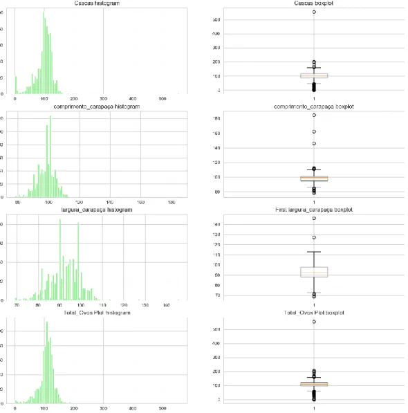
4.2.1 Outlier removal
Given I am running the data set though a set of algorithms that will look to learn interesting patterns in data, it is important to consider the existence of extreme or nonsense values that may exist in our data. Specifically, I am referring to values that could induce our algorithms into learning uninteresting patterns that lead to poor feature selection. Failure to do so, could have as a direct consequence the establishment of poor predictors and undermine the whole analysis. That being said, below are the histogram and boxplot graphical views for the variables where outliers were removed. The reasoning behind each selection is given after the graphics: