ABSTRACT: The variability within rows of cultivation may reduce the accuracy of experiments conducted in a complete randomized block design if the rows are considered as blocks, however, little is known about this variability in protected environments. Thus, our aim was to study the variability of the fresh mass in lettuce shoot, growing in protected environment, and to verify the border effect and size of the experimental unit in minimizing the productive variability. Data from two uniformity trials carried out in a greenhouse in autumn and spring growing seasons were used. In the statistical analyses, it was considered the existence of parallel cultivation rows the lateral openings of the greenhouse and of columns perpendicular to these openings. Different scenarios were simulated by excluding rows and columns to generate several borders arrangements and
BASIC AREAS -
Article
Variability, plot size and border effect in lettuce
trials in protected environment
Daniel Santos, Alessandro Dal’Col Lúcio*, Alberto Cargnelutti Filho, Sidinei José Lopes, Tiago Olivoto
Universidade Federal de Santa Maria – Departamento de Fitotecnia – Santa Maria (RS), Brazil.
*Corresponding author: adlucio@ufsm.br
Received: Mar. 15, 2017 – Accepted: Aug. 14, 2017
also to use different sizes of the experimental unit. For each scenario, homogeneity test of variances between remaining rows and columns was performed, and it was calculated the variance and coefficient of variation. There is variability among rows in trials with lettuce in plastic greenhouses and the border use does not bring benefits in terms of reduction of the coefficient of variation or minimizing the cases of heterogeneous variances among rows. In experiments with lettuce in a plastic greenhouse, the use of an experimental unit size greater than or equal to two plants provides homogeneity of variances among rows and columns and, therefore, allows the use of a completely randomized design.
INTRODUCTION
In 2013, the area planted with horticultural crops in Brazil achieved 800,1 thousand hectares, reaching a total production of ~18.8million tons (IBGE 2014). Among these crops, lettuce stands out as the most consumed leafy vegetables in Brazil, reaching more than 14 million plants cultivated in 2013, with a crescent increase each year (Santos 2015). Despite, there is still demand for growth of this crop in the country, since the consumption of vegetables in Brazil still does not correspond to that recommended by the World Health Organization.
Vegetable production has been oscillating over the years influenced, among other factors, by climatic adversities (Reetz et al. 2014). An efficient way of minimizing the effects of climatic adversities and obtaining stable lettuce production throughout the year is the use of protected environments (Goto 1997), a crescent alternative in Brazil.
Protected environments may be as, or more hetero- geneous as natural environments due to the variation in micrometeorological conditions that may occur within the protected environment, provided by its specific structural characteristics (Santos et al. 2010; Lúcio et al. 2011). In addition, characteristics inherent to horticultural crops such as the presence or absence of fruits suitable for harvesting, the multiple harvests that are carried out in some crops, and the more intensive cultural management in relation to other crops, are additional sources of variability (Lorentz et al. 2005; Lúcio et al. 2008). Thus, in this type of experiment, often strategies to reduce experimental error such as the use of concomitant observations, adequate experimental design, selection of the experimental unit size and shape, choice of sample size and number of replications cannot be used due to space limitations, or even when used, satisfactory results are not obtained. In these cases, the experiments do not present the necessary precision in order to adequately identify the differences between treatments.
Studies on reduction of experimental error in experiments with lettuce are restricted basically to the determination of sample size, experimental unit and definition of the experimental design (Marodin et al. 2000; Santos et al. 2007; Santos et al. 2010; Lúcio et al. 2011). Among their conclusions, these authors verified the existence of heterogeneity of variances cases between rows in several trials, but the existence of variability between columns, which would be important
because this variability would mean that the cultivation’s rows are not homogeneous, was not tested.
The existence of variability among cultivation rows has justified the use of a randomized block design in experiments with lettuce growing in protected environments, using the cultivation rows as the blocks (Segovia et al. 1997; Plese et al. 1998; Carvalho and Tessarioli Neto 2005; Lúcio et al. 2013). The use of this strategy would be efficient to minimize the effect of row variability on the variance of the error, however, if the hypothesis of variability among columns arranged in the opposite direction of the rows is true, variability within the blocks may be occurring, inflating the variance of experimental error. Thus, it is important to carry out a more detailed study of the variability in protected environments cultivated with vegetables in order to provide a higher accuracy of the experiments in this situation.
The use of border in the experimental units is widespread in field experiments with the aim of reducing the competition among plots (Storck et al. 2016). In this point of view, several studies have been carried out to test the efficiency of this technique in different crops (Fernandes and Silva 1994; Costa and Zimmermann 1998; Ribeiro et al. 2001; Cargnelutti Filho et al. 2003; Oliveira et al. 2005). For horticultural crops, however, similar studies were not found. The use of border in protected environments could also minimize the interaction of the plants of the side rows or the end of rows, near the openings of the structures, with the external environment, perhaps minimizing the variability in these environments. However, no studies testing the efficiency of borders use in minimizing the variability in protected environment cultivated with horticultural crops were found in the literature.
In this context, the aim of this research was to study the variability of the fresh mass of lettuce growing in protected environment and to verify the size of the experimental unit and border effect in minimizing this variability.
MATERIAL AND METHODS
the year and subtropical from the thermal’s point of view (Heldwein et al. 2009). The soil is classified in the Brazilian System of Classification of Soils (Santos et al. 2006) as Dystrophic Red Argisol.
The experiments were conducted in greenhouses, one in the autumn and other in the spring, with the cultivar Vera. The plants were arranged in crop rows spaced at 1.0 m, without the use of mulching, with plant spacing at 0.35 m. In both experiments, six cultivation rows were used, each containing 48 plants, arranged parallel to the lateral openings of the greenhouse. The assessed variable was the shoot’s fresh matter mass of all the plants of each experiment.
The greenhouse used has following dimensions: 2.0 m height lateral jamb stud, 3.5 m height central jamb stud, 20 m long and 10 m wide, oriented in a north-south direction. The greenhouse cover was made with low-density polyethylene (LDPE) film, with a thickness of 150 microns and anti-UV additive.
In order to carry out the statistical analyses, the plants were considered in the cultivation rows, parallel to the lateral openings of the greenhouse, and also the same plants arranged in columns, perpendicular to the lateral openings of the greenhouse. For each row and column, the mean, variance and coefficient of variation were calculated, simulating different experimental unit sizes, multiples of the number of plants per row. In each situation, the normality of the data was tested by the Lilliefors test (Campos 1983), afterward, the homogeneity of row and column variances were tested by the Bartlett test (Bartlett 1937).
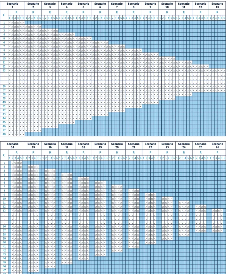
In order to verify the border effect on the variability, it was started from the original scenario (scenario 1) and new scenarios were created by the exclusion of rows (R) and columns (C) (Figure 1). To generate the new scenarios in all trials, a line was simultaneously excluded from each side end of the greenhouse. Columns were excluded one by one simultaneously at each end of the greenhouse up to 50% of the available columns has been excluded (Figure 1). The scenarios created were: 1) R0C0 – no border; 2) R0C1 – one column excluded; 3) R0C2 – two columns excluded; 4) R0C3 – three columns excluded; 5) R0C4 – four columns excluded; 6) R0C5 –five columns excluded; 7) R0C6 – six columns excluded; 8) R0C7 – seven columns excluded; 9) R0C8 – eight columns excluded; 10) R0C9 – nine columns
excluded; 11) R0C10 – ten columns excluded; 12) R0C11 – eleven columns excluded; 13) R0C12 – twelve columns excluded; 14) R1C0 – one row excluded; 15) R1C1 – one row and one column excluded; 16) R1C2 – one row and two columns excluded; 17) R1C3 – one row and three columns excluded; 18) R1C4 – one row and four columns excluded; 19) R1C5 – one row and five columns excluded; 20) R1C6 – one row and six columns excluded; 21) R1C7 – one row and seven columns excluded; 22) R1C8 – one row and eight columns excluded; 23) R1C9 – one row and nine columns excluded; 24) R1C10 – one row and ten columns excluded; 25) R1C11 – one row and eleven columns excluded; 26) R1C12 – one row and twelve columns excluded.
This procedure was performed at different experimental unit sizes, multiple of the number of plants per row. For each row or column exclusion or combination of row and column exclusion, and for each experimental unit size, a new variance was calculated per row and column, being the Lilliefors and Bartlett tests repeated. For each scenario, the variance and coefficient of variation of the experiment were calculated again. Statistical analyseswere performed in SAEG statistical software 9.1 and Microsoft Excel, with 5% error probability.
RESULTS AND DISCUSSION
By comparing the scenarios with exclusions of rows and/or columns (scenario 2 to 26) and the scenario with no
Figure 1. Scenarios created by the exclusion (highlighted in blue) of rows (R) and columns (C) in the greenhouse grown with lettuce.
Scenario 1 Scenario 2 Scenario 3 Scenario 4 Scenario 5 Scenario 6 Scenario 7 Scenario 8 Scenario 9 Scenario 10 Scenario 11 Scenario 12 Scenario 13
C R R R R R R R R R R R R R
1 2 3 4 5 6 1 2 3 4 5 6 1 2 3 4 5 6 1 2 3 4 5 6 1 2 3 4 5 6 1 2 3 4 5 6 1 2 3 4 5 6 1 2 3 4 5 6 1 2 3 4 5 6 1 2 3 4 5 6 1 2 3 4 5 6 1 2 3 4 5 6 1 2 3 4 5 6 1 × × × × × ×
2 × × × × × × × × × × × ×
3 × × × × × × × × × × × × × × × × × ×
4 × × × × × × × × × × × × × × × × × × × × × × × ×
5 × × × × × × × × × × × × × × × × × × × × × × × × × × × × × ×
6 × × × × × × × × × × × × × × × × × × × × × × × × × × × × × × × × × × × ×
7 × × × × × × × × × × × × × × × × × × × × × × × × × × × × × × × × × × × × × × × × × ×
8 × × × × × × × × × × × × × × × × × × × × × × × × × × × × × × × × × × × × × × × × × × × × × × × ×
9 × × × × × × × × × × × × × × × × × × × × × × × × × × × × × × × × × × × × × × × × × × × × × × × × × × × × × ×
10 × × × × × × × × × × × × × × × × × × × × × × × × × × × × × × × × × × × × × × × × × × × × × × × × × × × × × × × × × × × ×
11 × × × × × × × × × × × × × × × × × × × × × × × × × × × × × × × × × × × × × × × × × × × × × × × × × × × × × × × × × × × × × × × × × ×
12 × × × × × × × × × × × × × × × × × × × × × × × × × × × × × × × × × × × × × × × × × × × × × × × × × × × × × × × × × × × × × × × × × × × × × × × ×
13 × × × × × × × × × × × × × × × × × × × × × × × × × × × × × × × × × × × × × × × × × × × × × × × × × × × × × × × × × × × × × × × × × × × × × × × × × × × × × ×
. . . . . . . . . . . .
36 × × × × × × × × × × × × × × × × × × × × × × × × × × × × × × × × × × × × × × × × × × × × × × × × × × × × × × × × × × × × × × × × × × × × × × × × × × × × × ×
37 × × × × × × × × × × × × × × × × × × × × × × × × × × × × × × × × × × × × × × × × × × × × × × × × × × × × × × × × × × × × × × × × × × × × × × × × × × × × × ×
38 × × × × × × × × × × × × × × × × × × × × × × × × × × × × × × × × × × × × × × × × × × × × × × × × × × × × × × × × × × × × × × × × × ×
39 × × × × × × × × × × × × × × × × × × × × × × × × × × × × × × × × × × × × × × × × × × × × × × × × × × × × × × × × × × × ×
40 × × × × × × × × × × × × × × × × × × × × × × × × × × × × × × × × × × × × × × × × × × × × × × × × × × × × × ×
41 × × × × × × × × × × × × × × × × × × × × × × × × × × × × × × × × × × × × × × × × × × × × × × × ×
42 × × × × × × × × × × × × × × × × × × × × × × × × × × × × × × × × × × × × × × × × × ×
43 × × × × × × × × × × × × × × × × × × × × × × × × × × × × × × × × × × × ×
44 × × × × × × × × × × × × × × × × × × × × × × × × × × × × × ×
45 × × × × × × × × × × × × × × × × × × × × × × × ×
46 × × × × × × × × × × × × × × × × × ×
47 × × × × × × × × × × × ×
48 × × × × × ×
Scenario 14 Scenario 15 Scenario 16 Scenario 17 Scenario 18 Scenario 19 Scenario 20 Scenario 21 Scenario 22 Scenario 23 Scenario 24 Scenario 25 Scenario 26
C R R R R R R R R R R R R R
1 2 3 4 5 6 1 2 3 4 5 6 1 2 3 4 5 6 1 2 3 4 5 6 1 2 3 4 5 6 1 2 3 4 5 6 1 2 3 4 5 6 1 2 3 4 5 6 1 2 3 4 5 6 1 2 3 4 5 6 1 2 3 4 5 6 1 2 3 4 5 6 1 2 3 4 5 6 1 × × × ×
2 × × × × × × × ×
3 × × × × × × × × × × × ×
4 × × × × × × × × × × × × × × × ×
5 × × × × × × × × × × × × × × × × × × × ×
6 × × × × × × × × × × × × × × × × × × × × × × × ×
7 × × × × × × × × × × × × × × × × × × × × × × × × × × × ×
8 × × × × × × × × × × × × × × × × × × × × × × × × × × × × × × × ×
9 × × × × × × × × × × × × × × × × × × × × × × × × × × × × × × × × × × × ×
10 × × × × × × × × × × × × × × × × × × × × × × × × × × × × × × × × × × × × × × × ×
11 × × × × × × × × × × × × × × × × × × × × × × × × × × × × × × × × × × × × × × × × × × × ×
12 × × × × × × × × × × × × × × × × × × × × × × × × × × × × × × × × × × × × × × × × × × × × × × × ×
13 × × × × × × × × × × × × × × × × × × × × × × × × × × × × × × × × × × × × × × × × × × × × × × × × × × × ×
. . . . . . . . . . . .
36 × × × × × × × × × × × × × × × × × × × × × × × × × × × × × × × × × × × × × × × × × × × × × × × × × × × ×
37 × × × × × × × × × × × × × × × × × × × × × × × × × × × × × × × × × × × × × × × × × × × × × × × × × × × ×
38 × × × × × × × × × × × × × × × × × × × × × × × × × × × × × × × × × × × × × × × × × × × ×
39 × × × × × × × × × × × × × × × × × × × × × × × × × × × × × × × × × × × × × × × ×
40 × × × × × × × × × × × × × × × × × × × × × × × × × × × × × × × × × × × ×
41 × × × × × × × × × × × × × × × × × × × × × × × × × × × × × × × ×
42 × × × × × × × × × × × × × × × × × × × × × × × × × × × ×
43 × × × × × × × × × × × × × × × × × × × × × × × ×
44 × × × × × × × × × × × × × × × × × × × ×
45 × × × × × × × × × × × × × × × ×
46 × × × × × × × × × × × ×
47 × × × × × × × ×
48 × × × ×
allowed, in most cases, that the percentage of cases with variance heterogeneity between rows remained the same or increased (Table 1). In some situations of the spring experiment, the percentage of cases with heterogeneous variances between rows decreased, and in the scenarios 2, 3, 4, 5 and 6, the variances were homogeneous (Table 2). In some scenarios, however, the percentage of heterogeneous variance has increased.
As the results were not repeated between scenarios in the two growing seasons, it is not possible to make a
recommendation of the number of rows or columns to be excluded in order to provide homogeneous variances.
Regarding the number of plants per experimental unit, when there were no row or column exclusions (scenario 1), it was noticed that the increase in the size of the experimental unit was effective in reducing the cases of heterogeneity of variances between rows in both growing seasons (Tables 1 and 2). These results agree with Zhang et al. (1994), who verified that the increase of the size of the experimental unit provides a reduction of the variability. Thus, for
Scenario Size of experimental unit in plants
1 2 3 4 5 6 7 8 9 10
1 0.00 4.58 53.55 77.93 - 83.24 - 70.81 -
-2 0.00 23.95 - - -
-3 0.00 1.82 - 20.10 - - -
-4 0.00 5.74 14.38 - - 46.06 61.45 - -
-5 0.00 0.26 - 31.51 37.87 - - 68.16 - 73.38
6 0.00 7.34 - - -
-7 0.00 0.18 0.63 8.54 - 35.04 - - 38.02
-8 0.00 1.95 - - -
-9 0.00 0.09 - 22.67 - - - 21.58 -
-10 0.00 1.46 0.66 - 25.10 15.73 - - - 74.07
11 0.00 0.09 - 6.38 - - 62.36 - -
-12 0.00 8.75 - - -
-13 0.00 0.20 4.86 47.07 - 63.02 - 50.14 -
-14 0.00 4.51 40.36 60.67 - 58.07 - 53.05 -
-15 0.00 10.82 - - -
-16 0.00 0.80 - 14.13 - - -
-17 0.00 2.24 6.45 - - 21.05 35.25 - -
-18 0.00 0.06 - 16.00 17.17 - - 65.78 - 74.99
19 0.00 2.61 - - -
-20 0.00 0.04 0.35 3.03 - 71.59 - - 84.63
-21 0.00 1.19 - - -
-22 0.00 0.04 - 18.14 - - - 63.32 -
-23 0.00 0.72 0.35 - 11.22 6.53 - - - 97.19
24 0.00 0.03 - 2.06 - - 74.53 - -
-25 0.00 2.98 - - -
-26 0.00 0.18 1.47 21.69 - 75.80 - 41.73 -
-Table 1. Minimum level of significance of the Bartlett’s test (%) among lettuce rows in different scenarios created by the exclusion of rows and columns, in different experimental unit sizes for the experiment carried out in a greenhouse in autumn season.
lettuce crop, the use of an experimental unit constituted of a single plant is not recommended.
When no row or column deletions were made (scenario 1), the variances among columns, in opposite direction to the crop rows, were homogeneous in the two growing seasons (Tables 3 and 4). However, in some scenarios where exclusions were made, the variances among columns were heterogeneous. This result proves that column and/ or row deletion is not effective in the homogenization
of columns and, in some situations, it can make them heterogeneous.
The results found in this research allow us to verify that the use of borders composed of rows and/or columns is not effective in the homogenization of variances between rows or columns. This homogenization is achieved by increasing the size of the experimental unit. Thus, it is suggested that in these experiments it is possible to use the completely randomized design,
Scenario Size of experimental unit in plants
1 2 3 4 5 6 7 8 9 10
1 2.74 52.34 38.63 59.08 - 66.12 - 61.81 -
-2 7.76 24.65 - - -
-3 7.92 52.84 - 60.83 - - -
-4 15.66 32.35 54.77 - - 22.69 53.74 - -
-5 11.80 52.30 - 57.31 6.46 - - 36.31 - 44.79
6 13.89 32.89 - - -
-7 0.16 11.93 32.20 36.96 - 34.88 - - 49.58
-8 0.33 8.05 - - -
-9 0.47 19.05 - 43.97 - - - 39.39 -
-10 0.18 11.85 51.36 - 17.40 52.66 - - - 22.65
11 0.18 13.57 - 43.46 - - 74.22 - -
-12 0.39 14.84 - - -
-13 0.45 21.00 63.38 51.96 - 60.32 - 69.90 -
-14 18.20 38.22 30.09 36.62 - 68.81 - 70.35 -
-15 38.55 19.81 - - -
-16 42.36 45.27 - 82.54 - - -
-17 48.91 24.31 53.44 - - 26.10 37.74 - -
-18 46.03 58.44 - 49.81 43.07 - - 21.36 - 48.62
19 52.35 34.03 - - -
-20 0.19 6.98 26.03 36.72 - 50.49 - - 74.86
-21 0.36 3.79 - - -
-22 0.69 13.41 - 29.13 - - - 71.50 -
-23 0.49 6.85 37.10 - 49.74 46.85 - - - 53.35
24 0.77 13.08 - 51.57 - - 66.79 - -
-25 1.23 10.94 - - -
-26 1.60 19.50 50.80 37.00 - 65.70 - 44.95 -
-Table 2. Minimum level of significance of the Bartlett’s test (%) among lettuce rows in different scenarios created by the exclusion of rows and columns, in different experimental unit sizes for the experiment carried out in a greenhouse in spring season.
.
provided that a suitable experimental unit size be used.
In autumn and spring growing seasons, it was verified that the exclusion of only columns (scenarios 2 to 13) does not substantially changes the magnitude of the coefficient of variation (henceforth, CV). However, the exclusion of rows or rows jointly with columns (scenarios 14 to 26) reduces the CV, compared to the scenarios where these exclusions were not made (Tables 5 and 6). The reduction in CVs values, provided
by the exclusions, is related to the reduction of the means, since there are no significant changes in the magnitudes of variances. Lúcio et al. (2008) and Santos et al. (2012) point out that the lateral rows in protected environment are subjected to different conditions of air temperature and soil moisture. Possibly, the smallest CVs observed with the exclusion of lateral rows are due to the fact that these rows are in unfavorable conditions, with lower average production, and their exclusion has increased the average of the experiment, consequently reducing the CV.
Size of experimental unit in plants
Scenario 1 2 3 4 5 6 7 8 9 10
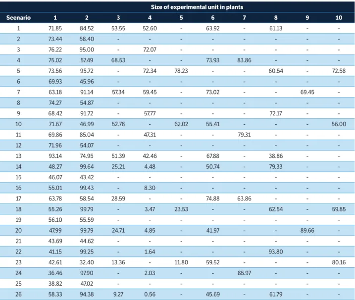
1 71.85 84.52 53.55 52.60 - 63.92 - 61.13 -
-2 73.44 58.40 - - -
-3 76.22 95.00 - 72.07 - - -
-4 75.02 57.49 68.53 - - 73.93 83.86 - -
-5 73.56 95.72 - 72.34 78.23 - - 60.54 - 72.58
6 69.93 45.96 - - -
-7 63.18 91.14 57.34 59.45 - 73.02 - - 69.45
-8 74.27 54.87 - - -
-9 68.42 91.72 - 57.77 - - - 72.17 -
-10 71.67 46.99 52.78 - 62.02 55.41 - - - 56.00
11 69.86 85.04 - 47.31 - - 79.31 - -
-12 71.96 54.07 - - -
-13 93.14 74.95 51.39 42.46 - 67.88 - 38.86 -
-14 48.27 99.64 25.21 4.48 - 50.74 - 79.33 -
-15 46.07 43.42 - - -
-16 55.01 99.43 - 8.30 - - -
-17 63.78 58.54 28.59 - - 74.88 63.86 - -
-18 55.26 99.79 - 3.47 23.53 - - 62.54 - 59.85
19 56.10 55.59 - - -
-20 47.99 99.79 24.71 4.85 - 41.97 - - 89.66
-21 43.69 44.62 - - -
-22 41.15 99.25 - 1.64 - - - 93.80 -
-23 42.61 32.40 13.36 - 11.80 59.52 - - - 80.16
24 36.46 97.90 - 2.03 - - 85.97 - -
-25 38.82 47.02 - - -
-26 58.33 94.38 9.27 0.56 - 45.69 - 61.79 -
-Table 3. Minimum level of significance of the Bartlett’s test (%) among lettuce columns in different scenarios created by the exclusion of rows and columns, in different experimental unit sizes for the experiment carried out in a greenhouse in autumn season.
The exclusion of lateral rows has reduced the CV, but in a discrete way and, as already discussed, this reduction was not reflected in the homogenization of rows or columns. Therefore, the exclusion of lateral rows in protected environments is not recommended, as it would also reduce the number of experimental units. The reduction of the number of experimental units would result in a reduction in the number of degrees of freedom of the error, impairing the accuracy of its estimation.
In scenario 1, the CV for the experimental unit composed of one plant was 42.14% in the autumn, while in the spring it was
33.72% (Table 5). These results show that the growing season influences the productive variability of horticultural crops and agrees with results found by Carpes et al. (2008; 2010), Lúcio et al. (2008; 2011), and Santos et al. (2010). This because the plants are exposed to different development conditions with the change of season, in addition, these different conditions can occur within the same season or vary in the same season from year to year. Thus, from the statistical-experimental point of view, it is not possible to indicate a seasonal season more suitable for experiments with lettuce in protected environment.
Scenario Size of experimental unit in plants
1 2 3 4 5 6 7 8 9 10
1 13.48 55.25 19.49 20.96 - 12.91 - 14.00 -
-2 11.40 51.30 - - -
-3 13.64 52.00 - 34.73 - - -
-4 22.50 94.07 35.13 - - 21.48 55.43 - -
-5 18.25 66.59 - 22.03 6.20 - - 29.92 - 46.83
6 18.39 94.11 - - -
-7 14.53 62.69 84.61 84.11 - 77.75 - - 78.44
-8 12.18 93.94 - - -
-9 19.44 71.00 - 71.64 - - - 57.72 -
-10 17.40 92.72 85.01 - 76.84 68.40 - - - 57.26
11 17.69 61.36 - 67.89 - - 66.31 - -
-12 18.82 87.39 - - -
-13 24.62 67.51 74.90 60.09 - 64.44 - 55.82 -
-14 1.20 48.45 34.73 36.94 - 18.27 - 13.97 -
-15 0.96 85.03 - - -
-16 1.46 39.69 - 56.79 - - -
-17 2.36 95.17 46.61 - - 36.71 32.32 - -
-18 1.48 37.35 - 26.96 7.09 - - 13.78 - 10.97
19 1.70 90.89 - - -
-20 1.89 39.08 69.35 70.65 - 40.59 - - 30.26
-21 1.19 85.91 - - -
-22 1.55 35.94 - 41.56 - - - 19.43 -
-23 1.10 78.35 57.64 - 45.94 51.34 - - - 47.20
24 1.19 31.98 - 56.24 - - 30.67 - -
-25 5.59 86.23 - - -
-26 5.86 46.59 66.00 50.86 - 38.67 - 50.84 -
-Table 4.Minimum level of significance of the Bartlett’s test (%) among lettuce columns in different scenarios created by the exclusion of rows and columns, in different experimental unit sizes for the experiment carried out in a greenhouse in spring season.
Table 5. Variance (S2, in g2.104) and coefficient of variation (CV, in percentage) for mass of fresh matter of aerial part of lettuce in the in different
scenarios created by the exclusion of columns, in different sizes of experimental unit for the experiment carried out in a greenhouse in
autumn season.
....continue
Scenario Size of experimental unit in plants
1 2 3 4 5 6 7 8 9 10
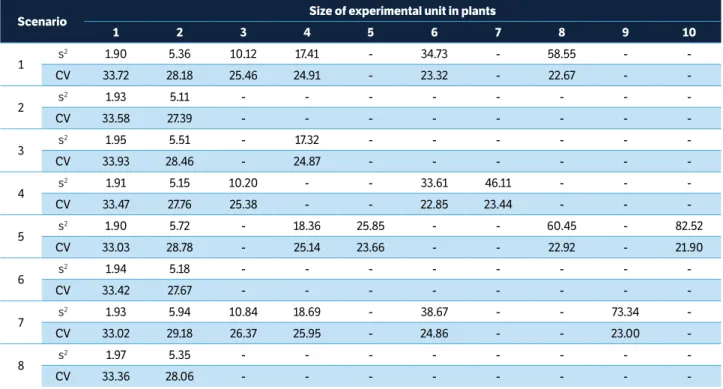
1 s
2 1.14 3.22 6.37 10.69 - 20.82 - 34.24 -
-CV 42.14 34.74 32.36 31.36 - 29.53 - 28.37 -
-2 s
2 1.10 3.15 - - - - - - -
-CV 41.03 34.10 - - -
-3 s
2 1.10 3.08 - 9.92 - - - - -
-CV 41.29 34.38 - 30.65 - - -
-4 s
2 1.08 3.09 5.97 - - 19.91 25.17 - -
-CV 40.97 34.06 31.66 - - 29.03 28.20 - -
-5 s
2 1.06 2.94 - 9.48 13.53 - - 33.16 - 48.07
CV 40.61 33.57 - 29.93 28.71 - - 28.01 - 27.32
6 s
2 1.07 3.05 - - - - - - -
-CV 40.63 33.62 - - -
-7 s
2 1.08 2.93 5.71 9.39 - 18.12 - - 37.61
-CV 40.75 33.45 30.83 29.65 - 27.95 - - 26.98
-8 s
2 1.04 2.93 - - - - - - -
-CV 40.39 33.25 - - -
-9 s
2 1.05 2.90 - 9.07 - - - 27.94 -
-CV 40.54 33.52 - 29.40 - - - 26.31 -
-10 s
2 1.09 3.07 5.80 - 13.40 19.31 - - - 44.62
CV 41.49 34.13 31.30 - 28.79 28.76 - - - 26.62
11 s
2 1.05 2.91 - 9.03 - - 21.23 - -
-CV 40.39 33.33 - 28.97 - - 26.18 - -
-12 s
2 0.99 2.67 - - - - - - -
-CV 39.57 31.62 - - -
-13 s
2 1.03 2.82 5.09 8.44 - 15.50 - 28.45 -
-CV 40.25 32.41 28.73 27.78 - 25.84 - 25.85 -
-14 s
2 0.98 2.49 4.56 7.42 - 13.21 - 21.64 -
-CV 35.25 27.54 23.54 21.80 - 20.69 - 20.20 -
-15 s
2 0.94 2.38 - - - - - - -
-CV 33.79 25.58 - - -
-16 s
2 0.97 2.51 - 7.66 - - - - -
-CV 34.62 27.59 - 22.84 - - -
-17 s
2 0.93 2.32 4.11 - - 13.06 15.54 - -
-CV 34.02 25.81 22.61 - - 20.69 19.26 - -
-18 s
2 0.93 2.28 - 6.39 8.90 - - 20.31 - 28.84
CV 33.70 26.38 - 19.96 19.59 - - 19.08 - 18.36
19 s
2 0.94 2.28 - - - - - - -
-Table 5. Continuation...
Scenarios: 1) R0C0 – no border; 2) R0C1 – one column excluded; 3) R0C2 – two columns excluded; 4) R0C3 – three columns excluded; 5) R0C4 – four columns excluded; 6) R0C5 – five columns excluded; 7) R0C6 – six columns excluded; 8) R0C7 – seven columns excluded; 9) R0C8 – eight columns excluded; 10) R0C9 – nine columns excluded; 11) R0C10 – ten columns excluded; 12) R0C11 – eleven columns excluded; 13) R0C12 – twelve columns excluded; 14) R1C0 – one row excluded; 15) R1C1 – one row and one column excluded; 16) R1C2 – one row and two columns excluded; 17) R1C3 – one row and three columns excluded; 18) R1C4 – one row and four columns excluded; 19) R1C5 – one row and five columns excluded; 20) R1C6 – one row and six columns excluded; 21) R1C7 – one row and seven columns excluded; 22) R1C8 – one row and eight columns excluded; 23) R1C9 – one row and nine columns excluded; 24) R1C10 – one row and ten columns excluded; 25) R1C11 – one row and eleven columns excluded; 26) R1C12 – one row and twelve columns excluded.
Scenario Size of experimental unit in plants
1 2 3 4 5 6 7 8 9 10
20 s
2 0.95 2.22 3.75 6.64 - 10.30 - - 20.53
-CV 33.94 25.90 21.02 20.61 - 17.79 - - 17.60
-21 s
2 0.92 2.20 - - - - - - -
-CV 33.77 24.72 - - -
-22 s
2 0.90 2.22 - 5.75 - - - 13.65 -
-CV 33.36 25.92 - 18.30 - - - 16.23 -
-23 s
2 0.94 2.25 3.79 - 8.25 11.58 - - - 22.52
CV 34.23 24.75 20.85 - 18.38 19.15 - - - 16.66
24 s
2 0.90 2.15 - 5.81 - - 9.30 - -
-CV 33.14 25.24 - 18.57 - - 15.07 - -
-25 s
2 0.85 1.77 - - - - - - -
-CV 32.79 22.33 - - -
-26 s
2 0.90 2.13 3.10 4.89 - 6.15 - 12.27 -
-CV 33.97 25.16 18.42 15.80 - 13.99 - 15.06 -
-Table 6. Variance (S2, in g2.104) and coefficient of variation (CV, in percentage) for mass of fresh matter of aerial part of lettuce in the in different scenarios created by the exclusion of columns, in different sizes of experimental unit for the experiment carried out in a greenhouse in spring season.
...continue
Scenario Size of experimental unit in plants
1 2 3 4 5 6 7 8 9 10
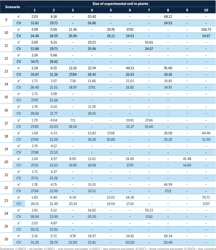
1 s
2 1.90 5.36 10.12 17.41 - 34.73 - 58.55 -
-CV 33.72 28.18 25.46 24.91 - 23.32 - 22.67 -
-2 s
2 1.93 5.11 - - - - - - -
-CV 33.58 27.39 - - -
-3 s
2 1.95 5.51 - 17.32 - - - - -
-CV 33.93 28.46 - 24.87 - - -
-4 s
2 1.91 5.15 10.20 - - 33.61 46.11 - -
-CV 33.47 27.76 25.38 - - 22.85 23.44 - -
-5 s
2 1.90 5.72 - 18.36 25.85 - - 60.45 - 82.52
CV 33.03 28.78 - 25.14 23.66 - - 22.92 - 21.90
6 s
2 1.94 5.18 - - - - - - -
-CV 33.42 27.67 - - -
-7 s
2 1.93 5.94 10.84 18.69 - 38.67 - - 73.34
-CV 33.02 29.18 26.37 25.95 - 24.86 - - 23.00
-8 s
2 1.97 5.35 - - - - - - -
-Table 6. Continuation...
Scenario Size of experimental unit in plants
1 2 3 4 5 6 7 8 9 10
9 s
2 2.03 6.18 - 20.42 - - - 68.12 -
-CV 33.81 29.73 - 26.86 - - - 24.53 -
-10 s
2 2.09 5.55 11.36 - 29.76 37.91 - - - 106.73
CV 34.46 28.55 26.96 - 26.13 24.53 - - - 24.67
11 s
2 2.05 6.21 - 19.23 - - 51.61 - -
-CV 33.88 29.73 - 25.96 - - 24.57 - -
-12 s
2 2.14 5.66 - - - - - - -
-CV 34.71 28.62 - - -
-13 s
2 2.24 6.72 12.16 22.74 - 44.13 - 76.40 -
-CV 35.87 31.26 27.84 28.42 - 26.53 - 26.18 -
-14 s
2 1.73 3.97 7.38 11.86 - 22.01 - 35.81 -
-CV 28.40 21.51 18.97 17.91 - 15.82 - 14.91 -
-15 s
2 1.73 3.98 - - - - - - -
-CV 27.97 21.66 - - -
-16 s
2 1.79 4.10 - 11.78 - - - - -
-CV 28.66 21.77 - 18.15 - - -
-17 s
2 1.70 4.04 7.11 - - 19.81 27.66 - -
-CV 27.80 22.03 18.50 - - 15.37 15.60 - -
-18 s
2 1.68 4.33 - 12.83 17.68 - - 38.08 - 44.46
CV 27.50 22.26 - 18.28 16.80 - - 15.35 - 13.30
19 s
2 1.74 4.12 - - - - - - -
-CV 27.98 22.10 - - -
-20 s
2 1.69 4.57 8.05 13.61 - 26.85 - - 41.48
-CV 27.10 22.63 19.95 19.58 - 17.74 - - 14.69
-21 s
2 1.73 4.27 - - - - - - -
-CV 27.31 22.26 - - -
-22 s
2 1.78 4.75 - 15.15 - - - 46.99 -
-CV 27.66 22.95 - 20.11 - - - 17.11 -
-23 s
2 1.83 4.40 8.39 - 22.01 24.38 - - - 70.71
CV 28.15 22.49 20.14 - 19.54 17.24 - - - 17.67
24 s
2 1.91 5.12 - 14.82 - - 35.23 - -
-CV 28.90 23.95 - 20.20 - - 17.62 - -
-25 s
2 2.03 4.87 - - - - - - -
-CV 30.21 23.91 - - -
-26 s
2 2.15 5.72 9.78 18.57 - 34.82 - 58.34 -
-CV 31.35 25.79 22.09 22.81 - 20.50 - 20.40 -
-.
CONCLUSION
The use of borders on the sides and ends of the rows inside the greenhouse does not bring benefits in terms of reducing the coefficient of variation or decreasing the cases of heterogeneity of variances among rows.
The use of an experimental unit size equal or greater than two plants in experiments with lettuce in greenhouses provides homogeneity of variances between rows and columns and, therefore, allows the use of completely randomized design.
ORCID IDs
D. Santos
https://orcid.org/0000-0003-3855-7480
A. D. Lúcio
https://orcid.org/0000-0003-0761-4200
A. Cargnelutti Filho
https://orcid.org/0000-0002-8608-9960
S. J. Lopes:
https://orcid.org/0000-0002-7117-541X
T. Olivoto
https://orcid.org/0000-0002-0241-9636
Bartlett, M. (1937). Properties of sufficiency and statistical tests. Proceeding of Royal Society of London. Ser. A, 160, 268-282. http:// dx.doi.org/10.1098/rspa.1937.0109.
Campos, H. (1983). Estatística experimental não-paramétrica. Piracicaba: ESALQ.
Cargnelutti Filho, A., Storck, L., Lúcio, A. D. C., Carvalho, M. P. and Santos, P. M. (2003). A precisão experimental relacionada ao uso de bordaduras nas extremidades das fileiras em ensaios de milho. Ciência Rural, 33, 607-614. http://dx.doi.org/10.1590/ S0103-84782003000400003.
Carpes, R. H., Lúcio, A. D. C., Lopes, S. J., Benz, V., Haesbaert, F. and Santos, D. (2010). Variabilidade produtiva e agrupamentos de colheitas de abobrinha italiana cultivada em ambiente protegido. Ciência Rural, 40, 264-271. http://dx.doi.org/10.1590/ S0103-84782010005000007.
Carpes, R. H., Lúcio, A. D. C., Storck, L., Lopes, S. J., Zanardo, B. and Paludo, A. L. (2008). Ausência de frutos colhidos e suas interferências na variabilidade da fitomassa de frutos de abobrinha italiana cultivada em diferentes sistemas de irrigação. Revista Ceres, 55, 590-595.
Carvalho, L. A. and Tessarioli Neto, J. (2005). Produtividade de tomate em ambiente protegido, em função do espaçamento e número de ramos por planta. Horticultura Brasileira, 23, 986-989. http://dx.doi.org/10.1590/S0102-05362005000400025. Costa, J. and Zimmermann, F. (1998). Efeitos de bordaduras laterais e de cabeceira no rendimento e altura de plantas de feijoeiro comum. Pesquisa Agropecuária Brasileira, 33, 297-304.
REFERENCES
Fernandes, A. and Silva, P. (1994). Efeito de bordadura nas extremidades de parcelas em experimentos com cultivares de milho. Caatinga, 8, 32-37.
Goto, R. (1997). Plasticultura nos trópicos: uma avaliação técnico-econômica. Horticultura Brasileira, 15, 163-165.
Heldwein, A., Buriol, G. and Streck, N. (2009). O clima de Santa Maria. Ciência & Ambiente, 38, 43-58.
Instituto Brasileiro de Geografia e Estatística. Levantamento sistemático da produção agrícola: pesquisa mensal de previsão de acompanhamento das safras agrícolas no ano civil. Rio de Janeiro: IBGE, 2014. Available at: ftp://ftp.ibge.gov.br/Producao_ Agricola/Levantamento_Sistematico_da_Producao_Agricola_ [mensal]/Fasciculo/2014/lspa_201401.pdf. Accessed on March 3, 2017.
Lorentz, L. H., Lúcio, A. D. C., Boligon, A. A., Lopes, S. J. and Storck, L. (2005). Variabilidade da produção de frutos de pimentão em estufa plástica. Ciência Rural, 35, 316-323. http://dx.doi.org/10.1590/ S0103-84782005000200011.
Lúcio, A. D. C., Carpes, R. H., Storck, L., Lopes, S. J., Lorentz, L. H. and Paludo, A.L. (2008). Variância e média da massa de frutos de abobrinha-italiana em múltiplas colheitas. Horticultura Brasileira, 26, 335-341. http://dx.doi.org/10.1590/ S0102-05362008000300009.
Lúcio, A. D. C, Schwertner, D. V, Santos, D., Haesbaert, F. M., Brunes, R. R. and Brackmann, A. (2013). Características produtivas e
morfológicas de frutos de tomateiro cultivado com bioproduto de
batata. Horticultura Brasileira, 31, 369-374. http://dx.doi.org/10.1590/ S0102-05362013000300005.
Marodim, V. S., Storck, L., Lopes, S. J., Santos, O. S. and Schimidt,
D. (2000). Delineamento experimental e tamanho de amostra para
alface cultivada em hidroponia. Ciência Rural, 30, 779-781. http:// dx.doi.org/10.1590/S0103-84782000000500006.
Oliveira, S. J. R., Feijó, S., Storck, L., Lopes, S. J., Martini, L. F. D. and
Damo, H.P. (2005). Substituindo o uso de bordaduras laterais por
repetições em experimentos com milho. Ciência Rural, 35, 10-15.
http://dx.doi.org/10.1590/S0103-84782005000100003. Plese, L. P. M., Tiritan, C. S., Yassuda, E. I., Prochnow, L. I., Corrente,
J. E. and Mello, S.C. (1998). Efeitos das aplicações de cálcio e de
boro na ocorrência de podridão apical e produção de tomate em
estufa. Scientia Agrícola, 55, 144-148. http://dx.doi.org/10.1590/ S0103-90161998000100023.
Reetz, E. R., Kist, B. B. and Santos, C. E. (2014). Anuário Brasileiro
de Hortaliças. Santa Cruz do Sul: Editora Gazeta.
Ribeiro, N. D., Storck, L. and Mello, R. M. (2001). Bordadura em
ensaios de competição de genótipos de feijoeiro relacionados
à precisão experimental. Ciência Rural, 31, 13-17. http://dx.doi. org/10.1590/S0103-84782001000100003.
Santos, C. E. (2015). Anuário Brasileiro de Hortaliças. Santa Cruz
do Sul: Editora Gazeta.
Santos, D., Haesbaert, F. M., Lúcio, A. D. C., Lopes, S. J., Cargnelutti Filho, A. and Benz, V., (2012). Aleatoriedade e variabilidade produtiva de feijão-de-vagem. Ciência Rural 42, 1147-1154. http://dx.doi. org/10.1590/S0103-84782012005000040.
Santos, D., Haesbaert, F. M., Puhl, O. J., Santos, J. R. A. and Lúcio, A. D. C. (2010). Suficiência amostral para alface cultivada em diferentes ambientes. Ciência Rural, 40, 800-805. http://dx.doi. org/10.1590/S0103-84782010000400009.
Santos, H. G., Jacomine, P. K. T., Anjos, L. H. C., Oliveira, V. A., Oliveira, J. B. Coelho, M. R., Lumbreras, J. F., and Cunha, T. J. F. (2006). Sistema Brasileiro de classificação de solos, Rio de Janeiro, EMBRAPA-SPI.
Santos, P. M. dos, Lopes, S. J., Lúcio, A. D. C., Santos, O. S., Santos, V. J. and Brum, B. (2007). Cronograma de amostragem de plantas de alface hidropônica para ajuste de curvas de crescimento. Ciência Rural, 37, 1601-1608. http://dx.doi.org/10.1590/ S0103-84782007000600015.
Segovia, J. F. O.,Andriolo, J. L., Buriol, G. A. and Schneider, F. M. (1997). Comparação do crescimento e desenvolvimento da alface (Lactucasativa L.) no interior e no exterior de uma estufa de polietilenoem Santa Maria, RS. Ciência Rural, 27, 37-41. http:// dx.doi.org/10.1590/S0103-84781997000100007.
Storck, L., Lopes, S., Estefanel, V. and Garcia, D. (2016). Experimentação Vegetal, 3.ed. Santa Maria: Editora UFSM.