AbstrAct: The objectives of this work were to determine the optimum plot size and number of repetitions to evaluate the fresh matter weight of vetch (Vicia sativa L.) in sowing densities. Forty-eight uniformity trials of 6 m × 6 m were conducted. Sixteen trials were evaluated in each sowing density (40, 60, and 80 kg∙ha−1). Each trial was divided into 36 basic experimental units (BEU) of 1 m × 1 m, totaling 1,728 BEU. In each BEU, the fresh matter was weighed. The optimum plot size was determined by the method of maximum curvature of the coefficient of variation model. The means were compared among sowing densities by the Scott-Knott’s test. The number of repetitions — for experiments with completely randomized and randomized block designs, in scenarios of i treatments
bAsic AreA -
Article
Plot size and number of repetitions in vetch
Alberto Cargnelutti Filho*, Bruna Mendonça Alves, Diego Nicolau Follmann, Cláudia Marques de Bem, Denison Esequiel Schabarum, Lucas da Silva Stefanelo, Cleiton Antonio Wartha, Jéssica Andiara Kleinpaul, Gabriela Görgen Chaves, Daniela Barbieri Uliana, Rafael Vieira Pezzini
Universidade Federal de Santa Maria - Departamento de Fitotecnia - Centro de Ciências Rurais - Santa Maria (RS), Brazil.
*Corresponding author: [email protected]
Received: Mar. 17, 2016 – Accepted: May 12, 2016
(i = 3, 4, …, 50) and d minimal differences between treatments means being detected as significant with 5% probability by Tukey’s test, expressed in percentage of the experiment average (d = 10%, 11%, …, 20%), was determined by iterative process until convergence. The optimum plot size to evaluate the fresh matter weight of vetch is 4.52 m2 at the 3 sowing densities. Four repetitions, to evaluate up to 50 treatments, in completely randomized and randomized block designs, are enough to identify as significant, at 5% probability by Tukey’s test, differences between treatment means of 29.15% of the experiment average.
iNtrODUctiON
The vetch (Vicia sativa L.) is an annual winter legume used as forage for animal feed and as cover crop (Santos et al. 2012). Researches with vetch, grown isolated or in mixture with other cover crops (Lithourgidis et al. 2006; Tuna and Orak 2007; Seidel et al. 2011; Ansar et al. 2013; Cherubin et al. 2014; Basbag et al. 2015; Desalegn and Hassen 2015), have demonstrated promising aspects of this crop. In isolated cultivation, in different environmental conditions, the fresh matter weights were 20.49 t∙ha−1
(Lithourgidis et al. 2006); 19.60 t∙ha−1 (Tuna and Orak
2007); 7.40 t∙ha−1 (Seidel et al. 2011); 11.13 t∙ha−1 (Ansar et
al. 2013); 25.94 t∙ha−1 (Cherubin et al. 2014); 18.32 t∙ha−1
(Basbag et al. 2015) and 14.833 t∙ha−1 (Desalegn and
Hassen 2015).
In studies with vetch, the experiments have presented variability in plot size, number of repetitions and sowing density. In vetch, oat and triticale cultivation in monoculture or in mixture, Lithourgidis et al. (2006) utilized plots of 100 m2 (20 × 5 m) and evaluated the
fresh matter weight in 30 m2 (10 × 3 m) of each plot.
Plots with 9 m2 (5 × 1.8 m) were used by Tuna and Orak
(2007) to evaluate the fresh matter weight of vetch and oat, grown isolated and in intercropping. In research of 3 cover crop species: black oat, turnip and vetch, besides a control treatment, Seidel et al. (2011) used 0.50 m2 per
plot (2 samples of 0.25 m2) in the determination of the
fresh matter weight. In pure and mixed cultivation with oat, wheat, vetch and barley, Ansar et al. (2013) used plots of 15 m2 and evaluated the fresh matter weight in
1 m2 of each plot.
Three samples of 0.25 m2 within each plot (0.75 m2)
were utilized to evaluate the fresh matter weight of vetch and other 6 cover crops (triticale, white oat, black oat, forage turnip, ryegrass and linseed), grown alone or in consortium (Cherubin et al. 2014). Nine species of vetch were studied in 7.2 m2 plots (6
× 1.2 m), being the
fresh matter weight evaluated in useful area of 3.0 m2
(5 × 0.6 m) (Basbag et al. 2015). In another experiment, the fresh matter weight of 4 vetch species was measured in plots of 6.0 m2 (6 × 1 m) (Desalegn and Hassen 2015).
These researches with vetch crop were performed in a randomized block design (RBD) with 3 (Tuna and Orak 2007; Ansar et al. 2013; Cherubin et al. 2014; Desalegn and Hassen 2015) and 4 repetitions (Lithourgidis
et al. 2006; Seidel et al. 2011; Basbag et al. 2015). Sowing densities of 170 kg∙ha−1 (Lithourgidis et al. 2006),
120 kg∙ha−1 (Tuna and Orak 2007), 45 kg∙ha−1 (Seidel
et al. 2011), 50 kg∙ha−1 (Ansar et al. 2013) and 30 kg∙ha−1
(Desalegn and Hassen 2015) were used. According to Santos et al. (2012), the vetch sowing density to be used varies from 40 to 60 kg∙ha−1.
In experiments with cover crops, such as vetch, it is important to quantify with precision the fresh matter weight in sowing densities. For this, sizing properly the plot size and the number of repetitions is essential to obtain reliable results of the treatments under evaluation. Based on data obtained in uniformity trials, it is possible to determine the optimum plot size by the method of maximum curvature of the coefficient of variation model (Paranaíba et al. 2009). In this method, it is necessary to estimate the first-order spatial autocorrelation coefficient, variance and mean as well as to calculate the optimum plot size based on these estimates. Then, based on the optimum plot size, it is possible to determine the number of repetitions in scenarios formed of combinations of treatments numbers, experimental precision and experimental designs. In this way, it is possible to establish the appropriate experimental design for the required precision, according to the experimental area, time, financial resources and labor availability.
Dimensioning the optimum plot size based on the method of maximum curvature of the coefficient of variation model (Paranaíba et al. 2009) and number of repetitions in combinations of treatments and precision levels have been carried out to measure fresh matter weight of cover crops, such as: black oat (Cargnelutti Filho et al. 2014a), jack bean (Cargnelutti Filho et al. 2014b), forage pea (Cargnelutti Filho et al. 2015a), canola (Cargnelutti Filho et al. 2015b), millet in evaluation times (Burin et al. 2015), millet in sowing and cut times (Burin et al. 2016) and pigeonpea (Santos et al. 2016). For these crops, the optimal plot size oscillated between 4.14 m2 for black oat
(Cargnelutti Filho et al. 2014a) and 8.39 m2 for pigeonpea
(Santos et al. 2016). In these studies, in addition to the plot size, it was dimensioned the number of repetitions in combinations of treatments and precision levels in completely randomized and randomized block designs, which are references for researches with these crops.
assess the fresh matter weight of vetch (Vicia sativa L.). Moreover, possible difference of plot size among sowing densities is unknown. These investigations can be carried out from uniformity trials data and can provide useful information to the appropriate experimental design. Thus, the objectives of this work were to determine the optimum plot size and number of repetitions and to evaluate the fresh matter weight of vetch (Vicia sativa L.) in sowing densities.
MAteriAL AND MetHODs
The uniformity trials (experiment without treatment, in which the crop and all procedures performed during the experiment are homogeneous throughout the experimental area) were carried out with vetch (Vicia sativa L.), common cultivar, in the experimental area located at lat 29°42′S, long 53°49′W and 95 m of altitude. According to Köppen, the climate is Cfa, humid subtropical, with hot summers and no dry season (Heldwein et al. 2009). The soil is classified as “Argissolo Vermelho distrófico arênico” Paleudalf (Santos et al. 2013). The sowing was broadcasted on May 13, 2015, within the indicated season to sow vetch, which extends from April to May (Santos et al. 2012), having been used the densities of 40, 60 and 80 kg∙ha−1 of seed. The following basic fertilization was
utilized: 20 kg∙ha−1 of N, 80 kg∙ha−1 of P
2O5 and 80 kg∙ha−1
of K2O. The cultural practices were conducted equally
throughout the experimental area, as recommended for uniformity trials (Storck et al. 2011; Ramalho et al. 2012). In the experimental area (75 × 40 m; 3,000 m2), 3 areas of
25 × 40 m (1,000 m2) were marked. The sowing densities
of 40, 60 and 80 kg∙ha−1 were held in the area 1, 2 and 3,
respectively. Sixteen uniformity trials with size of 6 m × 6 m (36 m2) were demarcated in each area (576 m2 of useful
area + 424 m2 of border area), totaling 48 uniformity trials
(3 areas × 16 uniformity trials per area). Each uniformity trial of size 6 m × 6 m (36 m2) was divided into 36 basic
experimental units (BEU) of 1 m × 1 m (1 m2), forming
a matrix with 6 rows and 6 columns. At 125 days after sowing, in the flowering vetch stage, the plants were cut close to the ground in each of the 1,728 BEU (3 areas × 16 uniformity trials per area × 36 BEU per uniformity trial) and the fresh matter weight (in g) was immediately weighed.
For each uniformity trial, the first-order spatial autocorrelation coefficient (ρ), the variance (s2), the mean (m), the coefficient of variation of the trial (CV, in %), the optimum plot size (Xo, in m2) and the coefficient
of variation in the optimum plot size (CVXo, in %) were
estimated with the fresh matter weight data of the 36 BEU. The ρ estimate was obtained in the rows, according to the methodology of Paranaíba et al. (2009) and application in Cargnelutti Filho et al. (2014a).
Based on the method of maximum curvature of the coefficient of variation model developed by Paranaíba et al. (2009), the optimum plot size
Xo = (103 √2(1-ρ2)s2m)/m
CVXo = (√(1-ρ2)s2/m2)/ √ Xo × 100
d = (qα(i;DFE)√MSE/r)/ m × 100
(1)
(2)
(3) and the coefficient of variation in the optimum plot size
were determined. The means comparisons of the statistics ρ, s2, m, CV, Xo and CVXo among the sowing densities were performed at 5% probability as follows: initially, the analysis of variance was performed (one-way, i.e. sowing density with 3 levels) via bootstrap with 10,000 resampling. Then, the 3 sowing densities were compared by Scott-Knott’s test via bootstrap with 10,000 resampling. In these analyzes, the trials were considered repetitions (independent samples, n = 16 trials at each sowing density). Analysis of variance and the Scott-Knott’s test via bootstrap were performed with Sisvar software (Ferreira 2014). According to Ferreira (2014), these statistical procedures are adequate to prevent possible impacts of non-compliance of the assumptions of normality of errors and homogeneity of residual variances.
In order to calculate the number of repetitions, it was initiated with the least significant difference (d) of the Tukey’s test, expressed as percentage of the experiment mean, which is estimated by the formula:
where: qα(i;DFE) is the critical value of the Tukey’s test at
RBD; MSE is the mean squared error; r is the number of repetitions; m is the experiment mean.
Thus, by replacing the expression of the coefficient of experimental variation
densities (large variability), allied with the appropriate plant development, it can be inferred that this database is suitable for the proposed study.
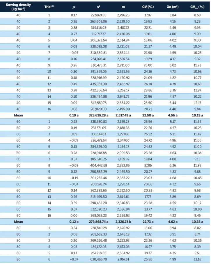
Regarding to the fresh matter weight of vetch, there was variability in the estimates of the first-order spatial autocorrelation coefficient (ρ), the variance (s2), the mean (m) and the coefficient of variation of the trial (CV), among 16 uniformity trials performed on each sowing density (40, 60 and 80 kg∙ha−1) (Table 1). In
this way, there was also variability in estimates of the optimum plot size (Xo) and the coefficient of variation in the optimum plot size (CVXo), whose estimates are
obtained based on ρ, s2 and m (Paranaíba et al. 2009). This wide variability scenario of ρ, s2, m, CV, Xo and CVXo statistics among 48 uniformity trials is important
for the properly dimensioning of plot size and number of repetitions. In field areas, this wide variability has also been observed in other cover crops, such as: black oat (Cargnelutti Filho et al. 2014a), jack bean (Cargnelutti Filho et al. 2014b), forage pea (Cargnelutti Filho et al. 2015a), canola (Cargnelutti Filho et al. 2015b), millet (Burin et al. 2015; Burin et al. 2016) and pigeonpea (Santos et al. 2016).
Among the 3 sowing densities, there was no significant difference between the means ρ, s2, CV, Xo and CVXo (Table 1). Wherefore, as Xo and CVXo did not differentiate
among sowing densities, the experimental design based on the overall average is an appropriate procedure to ensure the desired precision for these sowing densities. Thus, based on the average of 48 uniformity trials, it can be inferred that the optimum plot size to assess the fresh matter weight of vetch is 4.52 m² and the coefficient of variation in the optimum plot size was 10.10%, which is the base value to calculate the number of repetitions. Similar plot sizes to 4.52 m² were determined to evaluate the fresh matter weight of other cover crops. The determined sizes were: 4.14 m2 for black oat (Cargnelutti Filho et
al. 2014a), 5.85 m2 for jack bean (Cargnelutti Filho
et al. 2014b), 5.03 m2 for forage pea (Cargnelutti Filho et al.
2015a), 6.41 m2 for canola (Cargnelutti Filho et al. 2015b),
4.46 and 4.97 m2 for millet (Burin et al. 2015, Burin et al.
2016) and 8.39 m2 for pigeonpea (Santos et al. 2016).
In researches carried out by Lithourgidis et al. (2006), Tuna and Orak (2007) and Desalegn and Hassen (2015) to assess the fresh matter weight of vetch, the authors utilized plot sizes and useful area exceeding 4.52 m². CV = √MSE/m × 100
r = (qα(i; DFE) CV/d)2
(4)
(5) in percentage in the formula for the calculation of d and isolating r, it is obtained:
In the study, the CV is expressed as a percentage and corresponds to CVXo because this is the expected CV for the experiment with the determined optimum plot size (Xo).
From the average CVXo between the 3 sowing densities, the number of repetitions was determined (r) by iterative process until convergence, for experiments in completely randomized and randomized block designs, in scenarios formed by combinations of i (i = 3, 4, …, 50) and d [d = 10% (higher precision), 11%, …, 20% (lower precision)]. Statistical analyzes were performed using Microsoft®
Office Excel application and Sisvar software (Ferreira 2014).
resULts AND DiscUssiON
The fresh matter weight of vetch (Vicia sativa L.), common cultivar, oscillated between 22.11 and 27.96 t∙ha−1,
20.99 and 26.65 t∙ha−1, and 22.22 and 29.57 t∙ha−1,
respectively, for the sowing densities of 40, 60 and 80 kg∙ha−1 (Table 1). There was mean difference of fresh
matter weight of vetch between the 3 sowing densities. Detailed studies into the causes of these differences were not the focus of this research. The average of fresh matter weight of vetch among 48 uniformity trials (3 sowing densities × 16 uniformity trials per sowing density) was of 24.82 t∙ha−1 (Table 1). This average was greater than
that obtained by Seidel et al. (2011) (7.40 t∙ha−1), Ansar
et al. (2013) (11.13 t∙ha−1), Desalegn and Hassen (2015)
(14.833 t∙ha−1), Basbag et al. (2015) (18.32 t∙ha−1), Tuna and
Orak (2007) (19.60 t∙ha−1) and Lithourgidis et al. (2006)
(20.49 t∙ha−1). Also, it was smaller than that obtained by
Cherubin et al. (2014) (25.94 t∙ha−1). Therefore, in view
sowing density
(kg∙ha−1) trial
(1) ρ s2 m cV (%) Xo (m2) cV
Xo (%)
40 1 0.17 227,869.85 2,796.25 17.07 3.84 8.59
40 2 0.25 263,609.06 2,629.50 19.53 4.15 9.28
40 3 0.38 319,116.03 2,487.72 22.71 4.45 9.96
40 4 0.27 212,717.37 2,426.06 19.01 4.06 9.09
40 5 0.04 206,373.54 2,514.94 18.06 4.02 9.00
40 6 0.09 338,038.08 2,721.08 21.37 4.49 10.04
40 7 −0.05 310,380.81 2,534.14 21.98 4.59 10.25
40 8 0.16 234,076.41 2,507.64 19.29 4.17 9.32
40 9 0.25 330,475.31 2,211.00 26.00 5.02 11.23
40 10 0.30 391,869.05 2,591.56 24.16 4.73 10.58
40 11 0.18 338,916.99 2,420.92 24.05 4.82 10.77
40 12 0.49 435,981.00 2,465.97 26.78 4.78 10.69
40 13 0.28 422,356.54 2,252.17 28.86 5.35 11.97
40 14 0.10 336,454.88 2,641.75 21.96 4.57 10.22
40 15 0.09 542,589.78 2,584.22 28.50 5.44 12.17
40 16 0.08 267,020.00 2,495.00 20.71 4.40 9.84
Mean 0.19 a 323,615.29 a 2,517.49 a 22.50 a 4.56 a 10.19 a
60 1 0.22 338,930.83 2,159.28 26.96 5.17 11.56
60 2 0.19 237,371.09 2,188.36 22.26 4.57 10.23
60 3 0.09 333,147.83 2,227.06 25.92 5.11 11.42
60 4 −0.09 336,479.54 2,347.00 24.72 4.95 11.06
60 5 0.13 284,329.00 2,166.17 24.62 4.92 11.00
60 6 0.28 238,918.88 2,099.53 23.28 4.64 10.38
60 7 0.37 185,340.25 2,169.92 19.84 4.08 9.13
60 8 −0.09 404,442.58 2,283.86 27.85 5.36 11.98
60 9 0.12 250,585.29 2,469.50 20.27 4.33 9.68
60 10 −0.19 301,252.46 2,383.22 23.03 4.68 10.45
60 11 −0.04 200,178.24 2,228.14 20.08 4.32 9.66
60 12 0.14 262,892.66 2,522.50 20.33 4.33 9.68
60 13 0.26 215,495.50 2,614.61 17.75 3.89 8.69
60 14 0.39 298,482.20 2,316.83 23.58 4.55 10.17
60 15 0.07 322,020.23 2,386.94 23.77 4.83 10.80
60 16 0.00 268,033.23 2,665.53 19.42 4.23 9.45
Mean 0.12 a 279,868.74 a 2,326.78 b 22.73 a 4.62 a 10.33 a
80 1 0.34 238,849.28 2,626.92 18.60 3.94 8.82
80 2 0.08 209,582.33 2,643.19 17.32 3.91 8.74
80 3 0.30 269,556.48 2,222.92 23.36 4.63 10.35
80 4 0.03 189,122.03 2,673.03 16.27 3.75 8.39
80 5 0.13 257,218.65 2,564.92 19.77 4.25 9.51
80 6 −0.37 630,466.70 2,957.61 26.85 4.99 11.15
table 1. First-order spatial autocorrelation coefficient, variance, mean, coefficient of variation of the trial, optimum plot size, and coefficient of variation in the optimum plot size for fresh matter weight of vetch (Vicia sativa L.), common cultivar, in g∙m−2, in 48 uniformity trials (16 uniformity trials in each sowing density).
The plot sizes utilized by Ansar et al. (2013) (15 m2) and
by Basbag et al. (2015) (7.2 m2) were also higher than
4.52 m². However, the samples for evaluation of fresh matter weight of vetch were collected in areas smaller than 4.52 m². On the other hand, Seidel et al. (2011) and Cherubin et al. (2014) did not report the plot size. Although, the authors utilized 0.50 m2 (Seidel et al. 2011)
and 0.75 m2 per plot (Cherubin et al. 2014) to evaluate
the fresh matter weight, i.e. below the optimal plot size obtained in this study (4.52 m²).
The number of repetitions (r) of plots with 4.52 m2 for
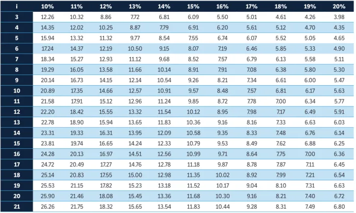
fixed number of treatments gradually increases with the decreasing of the least significant difference (d) (precision increase) in CRDs and RBDs (Tables 2,3). Smaller d estimates enable identifying minor differences between treatment means as significant and it signifies higher experimental precision (Lúcio et al. 1999; Storck et al. 2011). For least significant difference fixed percentage (d), the number of repetitions (r) of plots with 4.52 m2
increased with increasing number of treatments, regardless of the design (Tables 2,3). Wherefore, these results indicate that, for fixed plot size, the higher the required precision and the higher the number of treatments to be evaluated, the larger the number of repetitions.
For experiments in CRD, the number of repetitions (r) ranged from 3.98 for 3 treatments and precision of 20% (lower precision) to 32.66 repetitions for 50
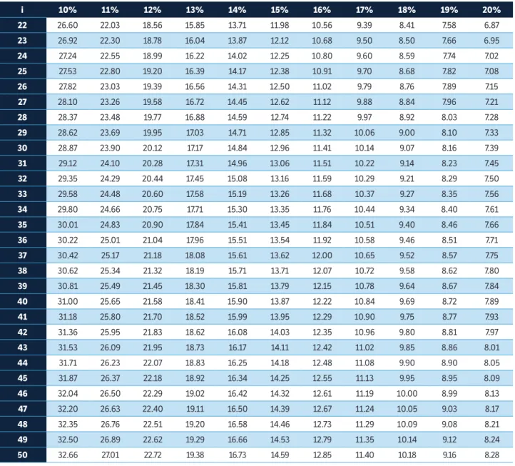
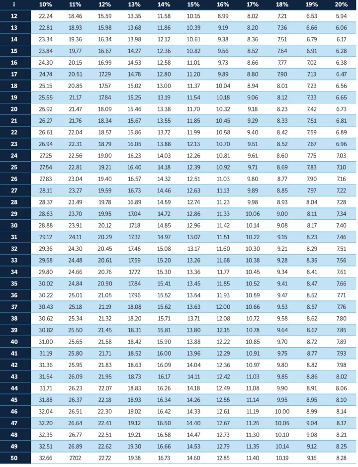
treatments and precision of 10% (higher precision) (Table 2). Moreover, for the experiments in RBDs, the number of repetitions oscillated from 4.42 (3 treatments and d = 20%) to 32.66 (50 treatments and d = 10%) (Table 3). Therefore, regardless of the experimental design, obtaining precision of 10% (higher precision) is impractical due to the elevated number of repetitions required. However, it is possible to establish the proper relations between i, d and the number of repetitions based on Xo = 4.52 m2.
In practice, to carry out the experiment, it is necessary to define the integer number of repetitions. Then, fixing r equal to 4 repetitions, as used in the experiments performed by Lithourgidis et al. (2006), Seidel et al. (2011) and Basbag et al. (2015), the least significant difference (d) of the Tukey’s test is estimated by the expression:
(1)Each uniformity trial of size 6 m × 6 m (36 m2) was divided into 36 basic experimental units of 1 m × 1 m (1 m2), forming a matrix with 6 rows and 6 columns; (2)For
each statistics (ρ, s2, m, CV, Xo, and CV
Xo), the means not followed by the same letter in column (comparison of means between sowing densities) differ at a 5%
probability by Scott-Knott’s test via bootstrap with 10,000 resampling. ρ = First-order spatial autocorrelation coefficient; s2 = Variance; m = Mean; CV = Coefficient
of variation of the trial; Xo = Optimum plot size; CVXo = Coefficient of variation in the optimum plot size. sowing density
(kg∙ha−1) trial
(1) ρ s2 m cV (%) Xo (m2) cV
Xo (%)
80 7 0.51 521,833.94 2,422.33 29.82 5.10 11.40
80 8 0.20 237,172.96 2,484.81 19.60 4.19 9.37
80 9 −0.19 235,899.26 2,681.33 18.11 3.98 8.91
80 10 −0.15 475,498.61 2,854.72 24.16 4.85 10.85
80 11 0.26 227,667.28 2,513.75 18.98 4.06 9.08
80 12 0.06 270,870.35 2,689.64 19.35 4.21 9.41
80 13 −0.41 312,779.69 2,568.17 21.78 4.29 9.60
80 14 0.00 458,435.45 2,590.92 26.13 5.15 11.52
80 15 −0.10 262,654.18 2,573.86 19.91 4.28 9.58
80 16 0.35 325,484.35 2,593.22 22.00 4.40 9.83
Mean 0.07 a 320,193.22 a 2,603.83 a 21.38 a 4.37 a 9.78 a
Overall mean 0.12 307,892.42 2,482.70 22.20 4.52 10.10
table 1. Continuation...
d = (qα(i;DFE)CV)/ √r
d = (q5%(20;60)× 10.10)/ √4 =
(5.2411998 × 10.10)/√4 = 26.47%
(6)
(7) expressed as percentage of the experiment average. Thus, with 20 treatments (number of usual treatments in experiments), for the CRD,
With 50 treatments (significant number of treatments), for the CRD,
d = (q5%(20;57)× 10.10)/ √4 =
(5.2533923 × 10.10)/√4 = 26.53%
d = (q5%(50;150)× 10.10)/ √4 =
(5.7710567 × 10.10)/√4 = 29.14%
d = (q5%(50;147)× 10.10)/ √4 = (5.7736023 × 10.10)/√4 = 29.15%
(8)
(9)
(10) and, for the RBD,
Then, it can be inferred that, to evaluate the fresh matter weight of vetch, in CRD and RBD with up to 50 treatments, 4 repetitions are enough to identify as significant, at 5% probability by Tukey’s test, differences between treatment means of 29.15% of the overall experiment average.
i 10% 11% 12% 13% 14% 15% 16% 17% 18% 19% 20%
3 12.26 10.32 8.86 7.72 6.81 6.09 5.50 5.01 4.61 4.26 3.98
4 14.35 12.02 10.25 8.87 7.79 6.91 6.20 5.61 5.12 4.70 4.35
5 15.94 13.32 11.32 9.77 8.54 7.55 6.74 6.07 5.52 5.05 4.65
6 17.24 14.37 12.19 10.50 9.15 8.07 7.19 6.46 5.85 5.33 4.90
7 18.34 15.27 12.93 11.12 9.68 8.52 7.57 6.79 6.13 5.58 5.11
8 19.29 16.05 13.58 11.66 10.14 8.91 7.91 7.08 6.38 5.80 5.30
9 20.14 16.73 14.15 12.14 10.54 9.26 8.21 7.34 6.61 6.00 5.47
10 20.89 17.35 14.66 12.57 10.91 9.57 8.48 7.57 6.81 6.17 5.63
11 21.58 17.91 15.12 12.96 11.24 9.85 8.72 7.78 7.00 6.34 5.77
12 22.20 18.42 15.55 13.32 11.54 10.12 8.95 7.98 7.17 6.49 5.91
13 22.78 18.90 15.94 13.65 11.83 10.36 9.16 8.16 7.33 6.63 6.03
14 23.31 19.33 16.31 13.95 12.09 10.58 9.35 8.33 7.48 6.76 6.14
15 23.81 19.74 16.65 14.24 12.33 10.79 9.53 8.49 7.62 6.88 6.25
16 24.28 20.13 16.97 14.51 12.56 10.99 9.71 8.64 7.75 7.00 6.36
17 24.72 20.49 17.27 14.76 12.78 11.18 9.87 8.78 7.87 7.11 6.45
18 25.14 20.83 17.55 15.00 12.98 11.35 10.02 8.92 7.99 7.21 6.54
19 25.53 21.15 17.82 15.23 13.18 11.52 10.17 9.04 8.10 7.31 6.63
20 25.90 21.46 18.08 15.45 13.36 11.68 10.30 9.16 8.21 7.40 6.72
21 26.26 21.75 18.32 15.65 13.54 11.83 10.44 9.28 8.31 7.49 6.80
In order to evaluate the fresh matter weight of other cover crops, in the same scenario, i.e. for experiments in CRD and RBD with 50 treatments and 4 repetitions, the least significant difference (d) varied among crops. Compared to d = 29.15% for vetch obtained in this study, lower values (higher precision) were obtained by Cargnelutti Filho et al. (2014a) for black oat (d = 26.7%), by Burin et al. (2016) for millet in sowing and cut times (d = 28.66%), and by Burin et al. (2015) for millet in evaluation times (d = 28.75%). On the other hand, higher values (lower precision) were obtained by Cargnelutti Filho et al. (2015a) for forage pea (d = 32.4%), by Cargnelutti Filho et al. (2014b) for jack bean (d = 37.78%), by Cargnelutti Filho et al. (2015b) for canola (d = 41.4%) and by Santos et al. (2016) for pigeonpea (d = 54.1%).
By definition, in any experiment which assesses fixed effect of treatments, the conclusions are valid for the conditions under which the experiment was carried out (Storck et al. 2011). Then, the experimental plan (plot size and number of repetitions) for a certain number of treatments, required precision, and experimental design
table 2. Number of repetitions, for experiments in completely randomized designs, in scenarios formed by combinations of i treatments (i = 3, 4,…, 50) and d minimal differences between treatments means being detected as significant with 5% probability by Tukey’s test, expressed in percentage of the experiment average (d = 10%, 11%, …, 20%), to evaluate the fresh matter weight of vetch (Vicia sativa L.), common cultivar, based on the optimum plot size (Xo = 4.52 m2) and coefficient of variation in the optimum plot size (CV
Xo = 10.10%).
i 10% 11% 12% 13% 14% 15% 16% 17% 18% 19% 20%
22 26.60 22.03 18.56 15.85 13.71 11.98 10.56 9.39 8.41 7.58 6.87
23 26.92 22.30 18.78 16.04 13.87 12.12 10.68 9.50 8.50 7.66 6.95
24 27.24 22.55 18.99 16.22 14.02 12.25 10.80 9.60 8.59 7.74 7.02
25 27.53 22.80 19.20 16.39 14.17 12.38 10.91 9.70 8.68 7.82 7.08
26 27.82 23.03 19.39 16.56 14.31 12.50 11.02 9.79 8.76 7.89 7.15
27 28.10 23.26 19.58 16.72 14.45 12.62 11.12 9.88 8.84 7.96 7.21
28 28.37 23.48 19.77 16.88 14.59 12.74 11.22 9.97 8.92 8.03 7.28
29 28.62 23.69 19.95 17.03 14.71 12.85 11.32 10.06 9.00 8.10 7.33
30 28.87 23.90 20.12 17.17 14.84 12.96 11.41 10.14 9.07 8.16 7.39
31 29.12 24.10 20.28 17.31 14.96 13.06 11.51 10.22 9.14 8.23 7.45
32 29.35 24.29 20.44 17.45 15.08 13.16 11.59 10.29 9.21 8.29 7.50
33 29.58 24.48 20.60 17.58 15.19 13.26 11.68 10.37 9.27 8.35 7.56
34 29.80 24.66 20.75 17.71 15.30 13.35 11.76 10.44 9.34 8.40 7.61
35 30.01 24.83 20.90 17.84 15.41 13.45 11.84 10.51 9.40 8.46 7.66
36 30.22 25.01 21.04 17.96 15.51 13.54 11.92 10.58 9.46 8.51 7.71
37 30.42 25.17 21.18 18.08 15.61 13.62 12.00 10.65 9.52 8.57 7.75
38 30.62 25.34 21.32 18.19 15.71 13.71 12.07 10.72 9.58 8.62 7.80
39 30.81 25.49 21.45 18.30 15.81 13.79 12.15 10.78 9.64 8.67 7.84
40 31.00 25.65 21.58 18.41 15.90 13.87 12.22 10.84 9.69 8.72 7.89
41 31.18 25.80 21.70 18.52 15.99 13.95 12.29 10.90 9.75 8.77 7.93
42 31.36 25.95 21.83 18.62 16.08 14.03 12.35 10.96 9.80 8.81 7.97
43 31.53 26.09 21.95 18.73 16.17 14.11 12.42 11.02 9.85 8.86 8.01
44 31.71 26.23 22.07 18.83 16.25 14.18 12.48 11.08 9.90 8.90 8.05
45 31.87 26.37 22.18 18.92 16.34 14.25 12.55 11.13 9.95 8.95 8.09
46 32.04 26.50 22.29 19.02 16.42 14.32 12.61 11.19 10.00 8.99 8.13
47 32.20 26.63 22.40 19.11 16.50 14.39 12.67 11.24 10.05 9.03 8.17
48 32.35 26.76 22.51 19.20 16.58 14.46 12.73 11.29 10.09 9.08 8.21
49 32.50 26.89 22.62 19.29 16.66 14.53 12.79 11.35 10.14 9.12 8.24
50 32.66 27.01 22.72 19.38 16.73 14.59 12.85 11.40 10.18 9.16 8.28
table 2. Continuation...
i 10% 11% 12% 13% 14% 15% 16% 17% 18% 19% 20%
3 12.75 10.82 9.34 8.20 7.30 6.58 5.99 5.48 5.09 4.72 4.42
4 14.63 12.30 10.53 9.16 8.07 7.20 6.48 5.89 5.39 4.98 4.62
5 16.13 13.50 11.50 9.95 8.72 7.73 6.93 6.26 5.70 5.23 4.83
6 17.38 14.51 12.32 10.63 9.29 8.21 7.32 6.59 5.98 5.47 5.03
7 18.44 15.37 13.03 11.22 9.78 8.62 7.67 6.89 6.23 5.68 5.21
8 19.37 16.12 13.66 11.74 10.21 8.99 7.99 7.16 6.46 5.88 5.38
9 20.20 16.80 14.21 12.20 10.60 9.32 8.27 7.40 6.67 6.06 5.54
10 20.94 17.40 14.71 12.62 10.96 9.62 8.53 7.62 6.87 6.23 5.68
11 21.62 17.95 15.17 13.00 11.28 9.90 8.77 7.83 7.04 6.38 5.82
table 3. Number of repetitions, for experiments in randomized block designs, in scenarios formed by combinations of i treatments (i = 3, 4, …, 50) and d minimal differences between treatments means being detected as significant with 5% probability by Tukey’s test, expressed in percentage of the experiment average (d = 10%, 11%, …, 20%), to evaluate the fresh matter weight of vetch (Vicia sativa L.), common cultivar, based on the optimum plot size (Xo = 4.52 m2) and coefficient of variation in the optimum plot size (CV
Xo = 10.10%).
table 3. Continuation...
i 10% 11% 12% 13% 14% 15% 16% 17% 18% 19% 20%
12 22.24 18.46 15.59 13.35 11.58 10.15 8.99 8.02 7.21 6.53 5.94
13 22.81 18.93 15.98 13.68 11.86 10.39 9.19 8.20 7.36 6.66 6.06
14 23.34 19.36 16.34 13.98 12.12 10.61 9.38 8.36 7.51 6.79 6.17
15 23.84 19.77 16.67 14.27 12.36 10.82 9.56 8.52 7.64 6.91 6.28
16 24.30 20.15 16.99 14.53 12.58 11.01 9.73 8.66 7.77 7.02 6.38
17 24.74 20.51 17.29 14.78 12.80 11.20 9.89 8.80 7.90 7.13 6.47
18 25.15 20.85 17.57 15.02 13.00 11.37 10.04 8.94 8.01 7.23 6.56
19 25.55 21.17 17.84 15.25 13.19 11.54 10.18 9.06 8.12 7.33 6.65
20 25.92 21.47 18.09 15.46 13.38 11.70 10.32 9.18 8.23 7.42 6.73
21 26.27 21.76 18.34 15.67 13.55 11.85 10.45 9.29 8.33 7.51 6.81
22 26.61 22.04 18.57 15.86 13.72 11.99 10.58 9.40 8.42 7.59 6.89
23 26.94 22.31 18.79 16.05 13.88 12.13 10.70 9.51 8.52 7.67 6.96
24 27.25 22.56 19.00 16.23 14.03 12.26 10.81 9.61 8.60 7.75 7.03
25 27.54 22.81 19.21 16.40 14.18 12.39 10.92 9.71 8.69 7.83 7.10
26 27.83 23.04 19.40 16.57 14.32 12.51 11.03 9.80 8.77 7.90 7.16
27 28.11 23.27 19.59 16.73 14.46 12.63 11.13 9.89 8.85 7.97 7.22
28 28.37 23.49 19.78 16.89 14.59 12.74 11.23 9.98 8.93 8.04 7.28
29 28.63 23.70 19.95 17.04 14.72 12.86 11.33 10.06 9.00 8.11 7.34
30 28.88 23.91 20.12 17.18 14.85 12.96 11.42 10.14 9.08 8.17 7.40
31 29.12 24.11 20.29 17.32 14.97 13.07 11.51 10.22 9.15 8.23 7.46
32 29.36 24.30 20.45 17.46 15.08 13.17 11.60 10.30 9.21 8.29 7.51
33 29.58 24.48 20.61 17.59 15.20 13.26 11.68 10.38 9.28 8.35 7.56
34 29.80 24.66 20.76 17.72 15.30 13.36 11.77 10.45 9.34 8.41 7.61
35 30.02 24.84 20.90 17.84 15.41 13.45 11.85 10.52 9.41 8.47 7.66
36 30.22 25.01 21.05 17.96 15.52 13.54 11.93 10.59 9.47 8.52 7.71
37 30.43 25.18 21.19 18.08 15.62 13.63 12.00 10.66 9.53 8.57 7.76
38 30.62 25.34 21.32 18.20 15.71 13.71 12.08 10.72 9.58 8.62 7.80
39 30.82 25.50 21.45 18.31 15.81 13.80 12.15 10.78 9.64 8.67 7.85
40 31.00 25.65 21.58 18.42 15.90 13.88 12.22 10.85 9.70 8.72 7.89
41 31.19 25.80 21.71 18.52 16.00 13.96 12.29 10.91 9.75 8.77 7.93
42 31.36 25.95 21.83 18.63 16.09 14.04 12.36 10.97 9.80 8.82 7.98
43 31.54 26.09 21.95 18.73 16.17 14.11 12.42 11.03 9.85 8.86 8.02
44 31.71 26.23 22.07 18.83 16.26 14.18 12.49 11.08 9.90 8.91 8.06
45 31.88 26.37 22.18 18.93 16.34 14.26 12.55 11.14 9.95 8.95 8.10
46 32.04 26.51 22.30 19.02 16.42 14.33 12.61 11.19 10.00 8.99 8.14
47 32.20 26.64 22.41 19.12 16.50 14.40 12.67 11.25 10.05 9.04 8.17
48 32.35 26.77 22.51 19.21 16.58 14.47 12.73 11.30 10.10 9.08 8.21
49 32.51 26.89 22.62 19.30 16.66 14.53 12.79 11.35 10.14 9.12 8.25
is valid for the location of the uniformity trial. However, considering the lack of research in this sense for the vetch crop, the information provided in this study is extremely important as a reference point for future experiments with vetch. Generalized conclusions for vetch crop may be performed from more uniformity trials with variation of other factors, such as: location, cultivar, species, sowing and harvest season.
cONcLUsiON
The optimum plot size to evaluate the fresh matter weight of vetch is 4.52 m2 at the 3 sowing densities.
Four repetitions, to evaluate up to 50 treatments, in completely randomized and randomized block designs, are enough to identify as significant, at 5% probability by Tukey’s test, differences between treatment means of 29.15% of the experiment average.
AcKNOWLeDGeMeNts
We thank the National Council for Scientific and Technological Development (CNPq), the Coordination for the Improvement of Higher Education Personnel (CAPES), and the Rio Grande do Sul Research Foundation (FAPERGS) for granting scholarships.
Ansar, M., Mukhtar, M. A., Sattar, R. S., Malik, M. A., Shabbir, G.,
Sher, A. and Irfan, M. (2013). Forage yield as affected by common
vetch in different seeding ratios with winter cereals in Pothohar
region of Pakistan. Pakistan Journal of Botany, 45, 401-408.
Basbag, M., Sayar, M. S., Aydin, A., Hosgoren, H. and Demirel, R.
(2015). Some agronomical and quality traits in nine vetch (Vicia
ssp.) species cultivated in Southeastern Anatolia, Turkey. Journal
of Agricultural and Natural Sciences, 2, 69-77.
Burin, C., Cargnelutti Filho, A., Alves, B. M., Toebe, M. and Kleinpaul,
J. A. (2016). Plot size and number of replicates in times of sowing
and cuts of millet. Revista Brasileira de Engenharia Agrícola
e Ambiental, 20, 119-127. http://dx.doi.org/10.1590/1807-1929/
agriambi.v20n2p119-127.
Burin, C., Cargnelutti Filho, A., Alves, B. M., Toebe, M., Kleinpaul,
J. A. and Neu, I. M. M. (2015). Plot size and number of repetitions
in evaluation times in millet crop. Bragantia, 74, 261-269. http://
dx.doi.org/10.1590/1678-4499.0465.
Cargnelutti Filho, A., Alves, B. M., Burin, C., Kleinpaul, J. A.,
Neu, I. M. M., Silveira, D. L., Simões, F. M., Spanholi, R. and
Medeiros, L. B. (2015a). Plot size and number of repetitions
in forage pea. Ciência Rural, 45, 1174-1182. http://dx.doi.
org/10.1590/0103-8478cr20141043.
Cargnelutti Filho, A., Alves, B. M., Burin, C., Kleinpaul, J. A.,
Silveira, D. L. and Simões, F. M. (2015b). Plot size and number
reFereNces
of repetitions in canola. Bragantia, 74, 176-183. http://dx.doi.
org/10.1590/1678-4499.0420.
Cargnelutti Filho, A., Alves, B. M., Toebe, M., Burin, C., Santos, G.
O., Facco, G., Neu, I. M. M. and Stefanello, R. B. (2014a). Plot size
and number of repetitions in black oat. Ciência Rural, 44,
1732-1739. http://dx.doi.org/10.1590/0103-8478cr20131466.
Cargnelutti Filho, A., Toebe, M., Burin, C., Alves, B. M., Neu, I. M.
M., Casarotto, G. and Facco, G. (2014b). Plot size and number
of replicates in jack bean. Ciência Rural, 44, 2142-2150. http://
dx.doi.org/10.1590/0103-8478cr20140317.
Cherubin, M. R., Fabris, C., Weirich, S. W., Rocha, E. M. T., Basso,
C. J., Santi, A. L. and Lamego, F. P. (2014). Agronomic performance
of maize in succession to cover crop species under no-tillage
system in Southern Brazil. Global Science and Technology, 7, 76-85.
Desalegn, K. and Hassen, W. (2015). Evaluation of biomass yield
and nutritional value of different species of vetch (Vicia). Academic
Journal of Nutrition, 4, 99-105.http://dx.doi.org/10.5829/idosi.
ajn.2015.4.3.96130.
Ferreira, D. F. (2014). Sisvar: a guide for its bootstrap procedures
in multiple comparisons. Ciência e Agrotecnologia, 38, 109-112.
http://dx.doi.org/10.1590/S1413-70542014000200001.
Heldwein, A. B., Buriol, G. A. and Streck, N. A. (2009). O clima de
Lithourgidis, A. S., Vasilakoglou, I. B., Dhima, K. V., Dordas, C. A.
and Yiakoulaki, M. D. (2006). Forage yield and quality of common
vetch mixtures with oat and triticale in two seeding ratios.
Field Crops Research, 99, 106-113. http://dx.doi.org/10.1016/j.
fcr.2006.03.008.
Lúcio, A. D., Storck, L. and Banzatto, D. A. (1999). Quality control
of cultivar competition experiments through the analysis of the
statistics employed. Pesquisa Agropecuária Gaúcha, 5, 99-103.
Paranaíba, P. F., Ferreira, D. F. and Morais, A. R. (2009). Optimum
experimental plot size: Proposition of estimation methods. Revista
Brasileira de Biometria, 27, 255-268.
Ramalho, M. A. P., Ferreira, D. F. and Oliveira, A. C. (2012).
Experimentação em genética e melhoramento de plantas.
Lavras: UFLA.
Santos, G. O., Cargnelutti Filho, A., Alves, B. M., Burin, C., Facco,
G., Toebe, M., Kleinpaul, J. A., Neu, I. M. M. and Stefanello, R. B.
(2016). Plot size and number of repetitions in pigeonpea. Ciência
Rural, 46, 44-52. http://dx.doi.org/10.1590/0103-8478cr20150124.
Santos, H. G., Jacomine, P. K. T., Anjos, L. H. C., Oliveira, V. A.,
Oliveira, J. B., Coelho, M. R., Lumbreras, J. F. and Cunha, T. J.
F. (2013). Sistema brasileiro de classificação de solos. 3. ed.
Brasília: Embrapa.
Santos, H. P., Fontaneli, R. S., Fontaneli, R. S. and Tomm, G.
O. (2012). Leguminosas forrageiras anuais de inverno. In R. S.
Fontaneli, H. P. Santos and R. S. Fontaneli (Eds.), Forrageiras para
integração lavoura-pecuária-floresta na região sul-brasileira (p.
305-320). Brasília: Embrapa.
Seidel, E. P., Spaki, A. P., Silva, S. C., Silva, L. P. E. and Costa, N. V.
(2011). Effect of cover crops in beans crop and weed management.
Varia Scientia Agrárias, 2, 107-118.
Storck, L., Garcia, D. C., Lopes, S. J. and Estefanel, V. (2011).
Experimentação vegetal. 3. ed. Santa Maria: UFSM.
Tuna, C. and Orak, A. (2007). The role of intercropping on yield
potential of common vetch (Vicia sativa L.)/oat (Avena sativaL.)
cultivated in pure stand and mixtures. Journal of Agricultural and