Pesq. agropec. bras., Brasília, v.48, n.2, p.132-140, fev. 2013 DOI: 10.1590/S0100-204X2013000200002
Simulating maize yield in sub‑tropical conditions
of southern Brazil using Glam model
Homero Bergamaschi(1), Simone Marilene Sievert da Costa(2), Timothy Robert Wheeler(3)
and Andrew Juan Challinor(4)
(1)Universidade Federal do Rio Grande do Sul, Caixa Postal 15100, CEP 91501‑970 Porto Alegre, RS, Brazil. E‑mail: homerobe@ufrgs.br (2)Instituto Nacional de Pesquisas Espaciais, Centro de Previsão de Tempo e Estudos Climáticos, CEP 12630‑000 Cachoeira Paulista, SP, Brazil. E‑mail: simone@cptec.inpe.br (3)University of Reading, PO Box 217, Reading RG6 6AH, UK. E‑mail: t.r.wheeler@reading.ac.uk (4)University of Leeds, Leeds LS2 9JT, UK. E‑mail: challinor@leeds.ac.uk
Abstract – The objective of this work was to evaluate the feasibility of simulating maize yield in a sub‑tropical region of southern Brazil using the general large area model (Glam). A 16‑year time series of daily weather data were used. The model was adjusted and tested as an alternative for simulating maize yield at small and large spatial scales. Simulated and observed grain yields were highly correlated (r above 0.8; p<0.01) at large scales (greater than 100,000 km2), with variable and mostly lower correlations (r from 0.65 to 0.87; p<0.1) at small
spatial scales (lower than 10,000 km2). Large area models can contribute to monitoring or forecasting regional
patterns of variability in maize production in the region, providing a basis for agricultural decision making, and Glam‑Maize is one of the alternatives.
Index terms: Zea mays, crop modeling, crop parameters, crop‑weather relationships.
Simulação do rendimento de milho em condições subtropicais
do Sul do Brasil por meio do modelo Glam
Resumo – O objetivo deste trabalho foi avaliar a viabilidade de se estimar a produção de milho numa região subtropical do Sul do Brasil por meio do “general large area model” (Glam). Foi utilizada uma série de 16 anos de dados meteorológicos diários. O modelo foi ajustado e testado como alternativa para simular rendimentos de milho em pequena e grande escala espacial. Os rendimentos de milho simulados e observados estiveram altamente correlacionados (R acima de 0,8; p<0,01) em grande escala (mais de 100.000 km2), e apresentaram
correlações variáveis e geralmente inferiores (R de 0,65 a 0,87; p<0,1) em pequena escala (menos de 10.000 km2). Modelos de grande escala podem contribuir para monitorar ou predizer padrões de variabilidade
na produção de milho na região, o que fornece uma base para tomadas de decisão, e o Glam‑Maize é uma alternativa.
Termos para indexação: Zea mays, modelagem, parâmetros de cultivo, relações clima‑cultivo.
Introduction
The sub‑tropical region of South America is responsible for the majority of soybean, wheat, maize, rice, coffee, and sugarcane production in Latin America. With the exception of rice, these crops are generally conducted in rainfed conditions, and the oscillation of productivity is usually intense due to irregular rainfall distribution. Therefore, simulation can be a useful tool for predicting crop productivity a season or more ahead (Coelho & Costa, 2010) and to investigate options for crop management (Challinor et al., 2005).
Many simulation studies of grain crop yield have been done in different sub‑tropical regions of South
Sentelhas, 2009). Several observational studies on soil‑plant‑atmosphere relations have also been done in recent decades in southern Brazil (Müller et al., 2005; Bergamaschi et al., 2006). These modeling and observational researches have focused on spatial scales ranging from field (smaller than 10,000 km2) to larger areas (greater than 100,000 km2).
The general large area model (Glam) is a large area process‑based crop model used for simulating yield of annual crops (Challinor et al., 2004). It has a low input data requirement for large‑scale applications and can directly accept large‑scale climate information from global and regional climate models. The model has been previously used to simulate groundnut (Challinor et al., 2004; Osborne et al., 2007) and wheat production (Sanai et al., 2007) The main hypothesis of this study is that the Glam model is robust enough to simulate grain yields at large areas, for different crops and climate conditions.
The objective of this work was to evaluate the feasibility of simulating maize yields in a sub‑tropical region of Southern Brazil using Glam with a 16‑year time series of daily weather data.
Materials and Methods
The study was carried out in the South of Brazil, in the state of Rio Grande do Sul (27.2° to 29.8°S and 51.2° to 56.0°W, at an altitude range of 0–1,380 m) (Figure 1). The state is one of the main maize producers in the country. During the study period (1998–2005), it was ranked as the third main producer, but changed to the sixth position in 2004–2006 (Companhia Nacional de Abastecimento, 2006). Maize (Zea mays L.) yield was simulated at three spatial scales: the main producer region (northern‑northwestern zone of the state), which accounted for 83% of the state maize production during the studied period (Instituto Brasileiro de Geografia e Estatística, 2006); 11 micro‑regions within the producer region; and one municipality within each micro‑region (Figure 1; Table 1).
Maize yield production data from 1990 to 2005 (16 years) were collected from the Brazilian Institute of Geography and Statistics (Instituto Brasileiro de Geografia e Estatística, IBGE). Most maize crops in the state of Rio Grande do Sul are sown from September to the beginning of November and harvested from January to the beginning of March. The average sowing date for each municipality, obtained from
the data of the official extension service in the state (Emater, RS), represents the average date by which at least 50% of the maize crops were sown between 2002 and 2005. Once the sowing data was known, the mean date of tasseling, milky and physiological maturity was obtained from a set of experimental data (Matzenauer et al., 1995; Müller et al., 2005; Bergamaschi et al., 2006) for short season maize hybrids (Table 1).
Daily rainfall, global solar radiation, relative humidity, minimum and maximum air temperatures were taken in each of the 11 municipalities from 1990 to 2005. The same database was used for the municipality and the respective micro‑region (Figure 1). Weather data for the main producer region was the mean value of the 11 weather data stations. Weather stations belonged to the following official networks: Fundação Estadual de Pesquisa Agropecuária, Fepagro (in the municipalities of Cruz Alta, Erechim, Ijuí, Júlio de Castilhos, Santa Rosa, São Borja, Taquari, and Veranópolis) and Instituto Nacional de Meteorologia, Inmet (in the municipalities of Iraí, Passo Fundo, and São Luiz Gonzaga). Water retention data were taken from soil surveys (Dedececk, 197; Beltrame et al., 1979) of spatial units normally larger than one municipality. The prevailing soil type was used as the representative soil for each micro‑region. Average values of the 11 soil coefficients were calculated in order to provide a mean soil water condition of the whole producer region for: saturation, field capacity, and permanent wilting point.
Pesq. agropec. bras., Brasília, v.48, n.2, p.132‑140, fev. 2013
DOI: 10.1590/S0100‑204X2013000200002
The Glam processes and methodology were kept similar to the original framework, described by Challinor et al. (2004). A field experimental dataset
for maize was used to define new parameter values for Glam‑Maize in the region (Table 2). Great part of the data was obtained from field experiments carried
Table 1. Area of maize cultivation, average dates of sowing and phenological stages for each municipality, micro‑region, and main producer region.
Municipality Area (km2) Sowing date(1) Dates of the phenological stages(2) Period (days) from sowing to
Municipality Micro‑region Tasseling Milky maturity
Physiological maturity
Tasseling Physiological maturity
São Borja 3,627 12,986 12 Sep. 30 Nov. 30 Dec. 30 Jan. 79 140
São Luiz Gonzaga 1,292 7,860 12 Sep. 30 Nov. 30 Dec. 30 Jan. 79 140
Santa Rosa 489 3,336 22 Sep. 3 Dec. 2 Jan. 31Jan. 72 131
Ijuí 635 4,058 30 Sep. 9 Dec. 8 Jan. 8 Feb. 70 131
Iraí 200 1,393 20 Sep. 1 Dec. 31 Dec. 28 Jan. 72 130
Júlio de Castilhos 1,857 8,274 5 Oct. 10 Dec. 9 Jan. 10 Feb. 66 138
Cruz Alta 1,358 8,045 5 Oct. 10 Dec. 9 Jan. 10 Feb. 66 138
Passo Fundo 758 3,663 10 Oct. 17 Dec. 16 Jan. 7 Mar. 68 148
Erechim 426 2,349 10 Oct. 19 Dec. 18 Jan. 7 Mar. 70 148
Taquari 346 2,868 15 Oct. 22 Dec. 21 Jan. 22 Feb. 68 130
Veranópolis 276 1,469 21 Oct. 30 Dec. 29 Jan. 10 Mar. 70 140
Region 109,210 109,210 01 Oct. 14 Dec. 12 Jan. 12 Feb. 75 135
(1)Of at least 50% of the maize crops, according to the official extension service in the state(Emater, RS). (2)Mean date of tasseling, milky and physiological
maturity for short season maize hybrids (Matzenauer et al., 1995; Müller et al., 2005; Bergamaschi et al., 2006).
Table 2. Parameters and specific values used in the Glam model for simulating maize growth and yield in sub‑tropical conditions of southern Brazil.
Parameters Values Source
Growth and development Days from sowing to plant emergence 8 days Müller et al. (2005) Cardinal temperatures
Base, optimum(1), and maximum 8ºC, 32ºC (28–34), and 40ºC Kiniry (1991), Birch et al. (2003), Streck et al. (2009, 2012)
Thermal requirement
Stages 0, 1, 2, and 3 510, 580, 390, and 510 ºC‑day Müller et al. (2005) Leaf area index (L) rate (dL/dt)
Stages 0, 1, 2, and 3 0.025, 0.173, ‑0.017, and ‑0.050 per day Müller et al. (2005), Bergamaschi et al. (2006) Root growth (dLv/dL) 1.0 km cm‑1 m‑2 Adapted from Qin et al. (2006)
Root length density 0.38 cm cm‑3 Qin et al. (2006)
Harvest index (dH/dt) 0.0071 per day Müller (2001), Müller & Bergamaschi (2005) Soil water fraction threshold for L reduction 0.7 Bergamaschi et al (2006)
Evaporation and transpiration
Critical L for radiation interception 2.7 Bergamaschi et al. (2001), Radin et al. (2003) Maximum transpiration 0.63 cm per day Bergamaschi et al. (2001), Radin et al.(2003)
Transpiration efficiency 3.33 Pa Bergamaschi et al. (2001), Radin et al. (2003), Müller &
Bergamaschi (2005)
Maximum transpiration efficiency 4.7 Pa Bergamaschi et al. (2001), Radin et al. (2003), Müller &
Bergamaschi (2005)
Light extinction coefficient 0.46 Birch et al. (2003), Müller & Bergamaschi (2005)
Soil parameters and miscellaneous Field capacity(2)
Permanent wilting point Saturation
0.45 (0.25–0.51) 0.30 (0.17–0.36) 0.51 (0.33–0.59)
Dedececk (1974), Beltrame et al. (1979)
Soil water extraction front velocity 1.66 cm per day Müller (2001)
Soil water fraction for damage to anthesis 0.30 Bergamaschi et al. (2006)
Yield gap parameter 0.4–1.0 (varies spatially) Estimated by minimizing RMSE after yield calculation
(1)Data in parenthesis represent the range among authors. The parameter used in modeling was 32°C. (2)Field capacity at matrix potential of ‑0.006MPa (72
out in the state of Rio Grande do Sul in the 1980s and 1990s. Other parameters were obtained from the literature, with a preference for the most suitable to the regional cropping system (Table 2). All parameter values were kept constant across the study region, except for sowing dates, yield gap parameter, and soil water storage capacities. Sowing dates are given in Table 1. The yield gap parameter (YGP) accounts for the impacts on yield due to factors other than weather (i.e., pests, diseases, and management factors, which reduce yield by an amount referred to as the yield gap). The YGP was calculated by minimizing the root mean square error found between simulation and observation dataset, as proposed by Challinor et al. (2004).
The maize crop cycle was divided into four stages (Table 2): stage 0, juvenile stage, from sowing to four fully expanded leaves; stage 1, rapid vegetative growth, from the end of stage 0 to tasseling; stage 2, flowering, from tasseling to the beginning of grain‑filling; and stage 3, grain‑filling, from the end of stage 2 to physiological maturity. Plant emergence was assumed as occurring eight days from sowing. The duration of all other stages was determined using thermal time (degree‑days), calculated from the mean air temperature and cardinal temperatures (base, maximum, and optimum temperatures, Table 2). The thermal time chosen for each crop stage was in accordance with the experimental results for short season maize hybrids in the state. Those hybrids were assumed as photoperiod insensitive in the region.
The leaf area index growth rate (dL/dt) was based on a segmented linear model and varied for each stage (Table 2). The rate dL/dt increases from plant emergence to tasseling (stages 0 and 1) and decreases during stages 2 and 3. Those values were also taken from field experiments for short season maize hybrids, according to Müller et al. (2005).
Grain yield was calculated in Glam considering the above‑ground biomass and the harvest index (HI). The latter was simulated using a mean rate of change in the harvest index (dHI/dt) during the reproductive period, from tasseling to physiological maturity (stages 2 and 3), and it was based on a six‑year series of field experiments. Crop transpiration efficiency (TE) was calculated from the mean value of maximum evapotranspiration (ETm), measured in a weighing lysimeter, in five crop cycles (Bergamaschi et al., 2001; Radin et al., 2003). The partitioning of ETm to
transpiration and soil evaporation was obtained around the maximum leaf area index by measuring plant transpiration through sap flow using a heat pulse tracer (Santos et al., 2000).
Regression analysis of simulated yield against observations was done after any technology trend was removed, in order to test Glam‑Maize performance in simulating grain yield at the scale of municipalities, micro‑regions, and main producer region.
Results and Discussion
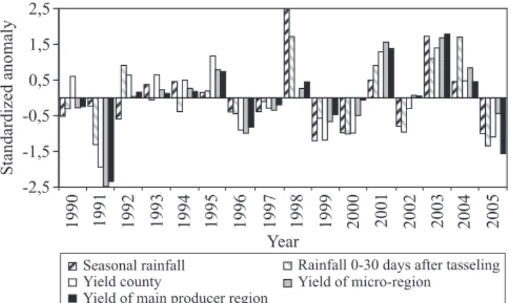
Variability indices of both grain yield and rainfall were calculated by dividing their anomalies (with respect to the historical mean) by the respective standard deviations (Figure 2). This normalized grain yield standardized anomaly tended to be larger for municipalities and micro‑regions than for the main producer region (Table 2). Rainfall during crop cycle explained (R2) more than one‑half of the detrended yield variance, whereas the rainfall during the 0–30 days after tasseling explained around 70% of the yield variance.
The effect of severe drought on grain yield is clearly shown in the 2004/2005 crop season, which was very dry; consequently, the harvest was less than half of that of the previous crop season (1,250 against 2,700 kg ha‑1 for 2003/2004). Soil water availability is particularly important for maize crops during the tasseling and silking stages, when the leaf area index
Pesq. agropec. bras., Brasília, v.48, n.2, p.132‑140, fev. 2013
DOI: 10.1590/S0100‑204X2013000200002
and the atmospheric evaporative demand are high (Bergamaschi et al., 2001, 2006; Radin et al., 2003). Tasseling occurred between December and January (Table 1). Therefore, short dry spells or isolated rainfall events during this period can cause high yield variability in maize crops in the region (Bergamaschi et al., 2006; Andriolli & Sentelhas, 2009). For example, the 1990/1991 season had a small rainfall anomaly for the entire crop cycle (i.e., standardized anomaly of ‑0.5, Figure 2), but a dry spell in the critical period of maize crops caused a strong negative effect in the 1990/1991 season (i.e., standardized anomaly of ‑1.25 for 0–30 days from tasseling). Since this short dry spell occurred in the critical period (tasseling to silking stages), a strong grain yield reduction was observed.
Some simulated and observed phenological events, as well as the leaf area index, are shown in Figure 3. The simulated data correspond to the municipality of Santa Rosa, whereas the observed data were measured at the Experimental Station of the Universidade Federal do Rio Grande do Sul (UFRGS), in the municipality of Eldorado do Sul, just outside of the main producer region, close to the Taquari micro‑region (Figure 1). Those two places have similar thermal conditions and a difference of about two degrees in latitude. However, limitations caused by water deficits in maize crops are higher in Eldorado do Sul than in Santa Rosa.
Glam‑Maize simulations of the time of the developmental stages were in good agreement with the observed data. Glam‑Maize estimated maximum leaf area index at 74 days after sowing, which was two days earlier than the observed data. The occurrence of milky maturity (102 days) and physiological maturity (132 days) was predicted five and one day later, respectively, than the observed. The agreement in timing (days after sowing) between estimated and observed phenological stages can be explained by the high dependence of maize phenology on the degree‑days accumulation, as observed by Streck et al. (2008). However, leaf area expansion showed a consistent lag between the simulated and observed data, which may be attributed to other factors. Since observed data were obtained from irrigated experiments, it is possible that water limitations in Santa Rosa (in rainfed conditions) promoted some delay in leaf area expansion. Because of the importance of the leaf area for solar radiation interception in crop modeling and of the complexity of the genotype x environment interactions on maize development in subtropical conditions (Streck et al., 2012), this aspect must be considered with extreme caution in adjusting and testing maize crops models.
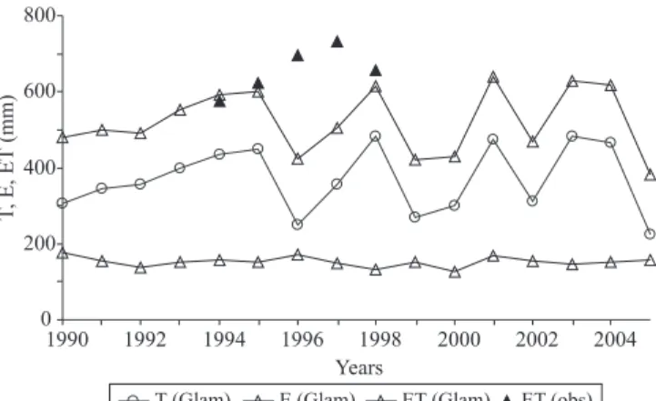
Glam‑Maize simulations of soil evaporation (E), crop evapotranspiration (ET) and transpiration (T) for the entire main producer region are presented in Figure 4. The total observed ET of irrigated maize measured with a weighing lysimeter, during five years,
Figure 3. Maize leaf area index averaged over six cropping seasons (1993/1994 to 1998/1999) from experimental data in Eldorado do Sul (solid lines) and simulated by the Glam model for the municipality of Santa Rosa (dashed lines), in the state of Rio Grande do Sul, Brazil. Vertical lines show the observed (solid lines) and simulated (dashed lines) dates of maximum leaf area index, milk maturity, and physiological maturity.
is also shown (Bergamaschi et al., 2001; Radin et al., 2003). Estimated ET was in good agreement with the experimental results during the three rainiest seasons (1994, 1995, and 1998). In contrast, the observed crop ET was higher than the ones simulated for the two years with substantial dry periods (1996 and 1997). This difference between observed and simulated ET can be mainly associated to the irrigation supply, which was not considered in the simulation.
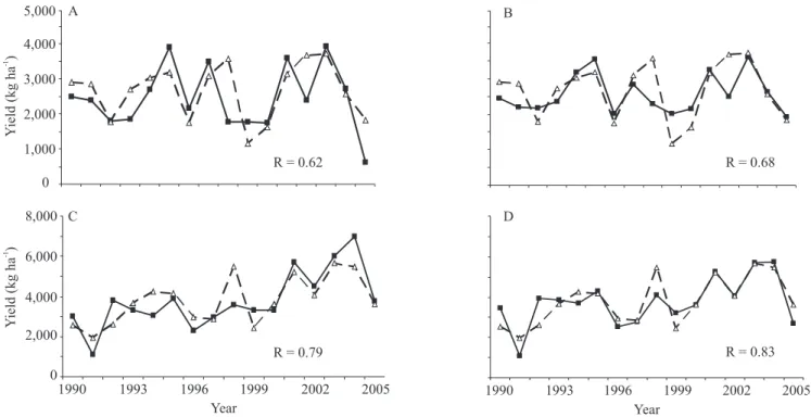
Simulated and observed maize yield time‑series for the municipalities of Santa Rosa and Passo Fundo and their respective micro‑regions are shown in Figure 5. These two micro‑regions showed different correlations between observed yield and rainfall (Figure 3). Time‑ series of observed and simulated crop yield for the main maize producer region are presented in Figure 6. Glam‑Maize simulated well the inter‑annual variability in maize yield for these time‑series, including those
Figure 5. Observed (■) and simulated (Δ) maize grain yields for the municipalities of Santa Rosa (A) and Passo Fundo (C) and their respective micro‑regions (B, D), in the state of Rio Grande do Sul, Brazil, from 1990 to 2005.
Pesq. agropec. bras., Brasília, v.48, n.2, p.132‑140, fev. 2013
DOI: 10.1590/S0100‑204X2013000200002
years with long drought periods, such as 2004/2005. The agreement between simulated and observed yields tended to increase from municipality to micro‑region, even though correlations between observed yield and rainfall did not show significant differences (Figure 2, Table 3). Glam‑Maize performance in simulating yield varied when the sowing date was changed, but these differences were not statistically significant (Table 4). Glam performance was analyzed under different spatial scales, technological levels, soil types, and sowing dates. The parameterizations in Glam are relatively simple, but complex enough to capture the climatic component of yield variability. The non‑climatic components include new plant genotypes, improvements in soil management and fertilization, and plant density (Berlato et al., 2005). Although possible variations in these factors were neglected (e.g., plant genotypes), Glam‑Maize simulated grain yield variability to a good degree of accuracy.
The comparison between observed and simulated yields is subject to constraints from both data and modeling. First, because a discrepancy (around 10%) between the two observed data sources (Conab and IBGE) for the same period (for the entire state) indicates a possible imprecision in the yield estimation methods of those official Brazilian agencies (Companhia Nacional de Abastecimento, 2006; Instituto Brasileiro de Geografia e Estatística, 2006). It is reasonable to expect that Glam‑Maize performance could be better analyzed with more accurate yield observations. Second, the wide range of sowing dates adopted by farmers (Table 2) is problematic for large‑area modeling. In the warmest zones, high thermal availability may sometimes permit two maize cycles in a single cropping season using very‑short season hybrids. Similarly, maize is sometimes sown on small farms just after the harvest of other spring crops, such as dry beans and tobacco, that delay the sowing of maize and reduce its potentiality. However, neither of these processes has been simulated in the present study. Third, regional variability in soil and topography may influence the spatial variability of hydrological conditions, and some regions have higher spatial variability in soils than others. For instance, the Santa Rosa micro‑region (site 5, Figure 1) has predominantly small farms and a mostly irregular pattern of soils and topography. In contrast, the Passo Fundo micro‑region (site 6, Figure 1), located in the northern plateau of the state, consists of medium to large farms with more uniform soils, topography, and technological levels. In this context, improvements in simulating water dynamics in the soil‑plant‑atmosphere system can be performed by matching the soil‑water storage to the observed conditions for each particular prevailing soil type.
Modeling maize yields in southern Brazil, even at large spatial scales, presents a great challenge, but can be very important for several applications, such as evaluating impacts of climatic changes on crops or estimating grain yield, taking seasonal climatic information as inputs. In this sense, Coelho & Costa (2010) observed a good performance of the Glam‑Maize model (parametrized in the present study) in simulating maize yields in southern Brazil by using seasonal climate forecasts. This study also shows that a process‑based model can simulate maize crop yield variability. A well‑designed model Table 3. Correlation coefficients between rainfall and
maize grain yields at three spatial scales: municipality, micro‑region, and main producer region, in the state of Rio Grande do Sul, Brazil.
Spatial scale Rainfall
Crop cycle (130–140 days)
0–30 days after tasseling
Municipality 0.52 0.67
Micro‑region 0.53 0.69
Main production region 0.56 0.72
Table 4. Correlation coefficients between simulated and observed yields of maize, for small and large spatial scales, with different sowing dates around the basic sowing date (BSD), from the 1989/1990 to the 2004/2005 cropping season, in the state of Rio Grande do Sul, Brazil.
Spatial scale Correlation coefficient(1)
BSD 10 days before BSD
10 days after BSD Small spatial scale
Santa Rosa municipality 0.69 0.65 0.73 Santa Rosa micro‑region 0.77 0.77 0.78 Passo Fundo municipality 0.71 0.71 0.72 Passo Fundo micro‑region 0.81 0.87 0.87
Large spatial scale
Main producer region 0.77 0.69 0.85
may produce accurate results when fitted and parametrized to regional cropping systems. For this purpose, a well‑established experimental basis seems to be indispensable, considering the complexity of the interactions among environmental factors on maize crops, in particular under sub‑tropical conditions (Streck et al., 2012), and the specificity in cropping systems. Further development of the Glam‑Maize model may improve its performance by introducing new adjustments that take into account short‑term water stresses around flowering time, when the number of grains is established (e.g., Ceres‑Maize model).
Conclusions
1. The general large area model for annual crops (Glam) captures the high inter‑annual variability of maize yield in the sub‑tropical conditions of the state of Rio Grande do Sul, Brazil, when parametrized for regional conditions and cropping systems.
2. Simulations of grain yields by the Glam‑Maize model are highly correlated with observed yields at large spatial scales, with variable correlations at smaller spatial scales.
3. Large area crop simulations by processed‑based models can contribute to monitoring or forecasting regional patterns of variability in maize yield in sub‑tropical conditions, providing a basis for agricultural decision making, and the Glam model is one of the alternatives.
Acknowledgements
To Conselho Nacional de Desenvolvimento Científico e Tecnológico (CNPq), for financial support; and to Fundação Estadual de Pesquisa Agropecuária (Fepagro), Instituto Nacional de Meteorologia (Inmet), Instituto Brasileiro de Geografia e Estatística (IBGE), Companhia Nacional de Abastecimento (Conab), Empresa de Assistência Técnica e Extensão Rural (Emater, RS), and Embrapa Trigo, for data on weather, maize production, phenology, and soil water.
References
ANDRIOLLI, K.G.; SENTELHAS, P.C. Brazilian maize genotypes
sensitivity to water deficit estimated through a simple crop yield
model. Pesquisa Agropecuária Brasileira, v.44, p.653‑660, 2009. DOI: 10.1590/S0100‑204X2009000700001.
BELTRAME, L.F.S.; TAYLOR, J.C.; CAUDURO, F.A. Probabilidade de ocorrência de déficits e excessos hídricos em
solos do Rio Grande do Sul. Porto Alegre: UFRGS, 1979. 79p.
BERGAMASCHI, H.; DALMAGO, G.A.; COMIRAN, F.; BERGONCI, J.I.; MÜLLER, A.G.; FRANÇA, S.; SANTOS, A.O.;
RADIN, B.; BIANCHI, C.A.M.; PEREIRA. P.G. Deficit hídrico
e produtividade na cultura do milho. Pesquisa Agropecuária
Brasileira, v.41, p.243‑249, 2006. DOI: 10.1590/S0100‑
204X2006000200008.
BERGAMASCHI, H.; RADIN, B.; ROSA, L.M.G.; BERGONCI, J.I.; ARAGONÉS, R.S.; SANTOS, A.O.; FRANÇA, S.; LANGENSIEPEN, M. Estimating maize water requirements using agrometeorological data. Revista Argentina de Agrometeorologia, v.1, p.23‑27, 2001.
BERLATO, M.A.; FARENZENA, H.; FONTANA, D.C. Associação entre El Niño Oscilação Sul e a produtividade do milho no Estado do Rio Grande do Sul. Pesquisa Agropecuária Brasileira, v.40, p.423‑432, 2005. DOI: 10.1590/S0100‑204X2005000500001.
BIRCH, C.J.; VOS, J.; VAN DER PUTTEN, P.E.L. Plant development and leaf area production in contrasting cultivars
of maize grown in a cool temperature environment in the field.
European Journal of Agronomy, v.19, p.173‑188, 2003. DOI:
10.1016/S1161‑0301(02)00034‑5.
CARDOSO, C.O.; FARIA, R.T. de; FOLEGATTI, M.V. Analysis of irrigation strategies for corn out season in Londrina with the Ceres maize model. Engenharia Agrícola, v.24, p.37‑45, 2004. DOI: 10.1590/S0100‑69162004000100005.
CHALLINOR, A.J.; WHEELER, T.R.; CRAUFURD, P.Q.; SLINGO, J.M.; GRIMES, D.I.F. Design and optimisation of a large area process based model for annual crops. Agricultural and Forest Meteorology, v.124, p.99‑120, 2004. DOI: 10.1016/j. agrformet.2004.01.002.
COELHO, C.A.S.; COSTA, S.M.S. Challenges for integrating seasonal climate forecasts in user applications. Current Opinion in Environmental Sustainability, v.2, p.317‑325, 2010. DOI: 10.1016/j.cosust.2010.09.002.
COMPANHIA NACIONAL DE ABASTECIMENTO. Companhia Nacional de Abastecimento [home page]. 2006. Disponível em:
<http://www.conab.gov.br>. Acesso em: 4 mar. 2013.
DEDECECK, R. Características físicas e fator de erodibilidade em oxissolos do Rio Grande do Sul. 1974. 132p. Dissertação (Mestrado) – Universidade Federal do Rio Grande do Sul, Porto Alegre.
DOORENBOS, J.; KASSAM, A.H. Yield response to water. Rome: FAO, 1979. 212p. (FAO. Irrigation and drainage paper, 33).
INSTITUTO BRASILEIRO DE GEOGRAFIA E ESTATÍSTICA.
Sistema IBGE de recuperação automática - SIDRA. 2006.
Disponível em: <http://www.sidra.ibge.gov.br>. Acesso em: 4 mar.
2013.
JENSEN, M.E. Water consumption by agricultural plants. In: KOZLOWSKY, T.T. (Ed.). Water deficits and plant growth. New York: Academic Press, 1968. v.2, p.1‑22.
Pesq. agropec. bras., Brasília, v.48, n.2, p.132‑140, fev. 2013
DOI: 10.1590/S0100‑204X2013000200002
MATZENAUER, R.; BERGAMASCHI, H.; BERLATO, M.A.; RIBOLDI, J. Modelos agrometeorológicos para estimativa do
rendimento de milho em função da disponibilidade hídrica no
Estado do Rio Grande do Sul. Pesquisa Agropecuária Gaúcha, v.1, p.225‑241, 1995.
MELLO, R.W. de; FONTANA, D.C.; BERLATO, M.A. Modelo agrometeorológico espectral de estimativa de rendimento da soja para o Estado do Rio Grande do Sul. In: SIMPÓSIO BRASILEIRO DE SENSORIAMENTO REMOTO, 11., 2003, Belo Horizonte.
Anais. Belo Horizonte: Inpe, 2003. p.172‑179.
MERCAU, J.L.; DARDANELLI, J.L.; COLLINO, D.J.; ADRIANI, J.M.; IRIGOYEN, A.; SATORRE, E.H. Predicting on farm soybean yields in pampas using CROPGRO soybean.
Field Crops Research, v.100, p.200‑209, 2007. DOI: 10.1016/j. fcr.2006.07.006.
MÜLLER, A.G. Modelagem da matéria seca e do rendimento
de grãos de milho em relação à disponibilidade hídrica. 2001. 120p. Tese (Doutorado) ‑ Universidade Federal do Rio Grande do Sul, Porto Alegre.
MÜLLER, A.G.; BERGAMASCHI, H. Eficiências de
interceptação, absorção e uso da radiação fotossinteticamente ativa pelo milho (Zea mays L.) em diferentes disponibilidades hídricas e verificação do modelo energético de estimativa da massa seca
acumulada. Revista Brasileira de Agrometeorologia, v.13, p.27‑ 33, 2005.
MÜLLER, A.G.; BERGAMASCHI, H.; BERGONCI, J.I.; RADIN,
B.; FRANÇA, S.; SILVA, M.I.G. Estimativa do índice de área
foliar do milho a partir da soma de graus dia. Revista Brasileira de Agrometeorologia, v.13, p.65‑71, 2005.
OSBORNE, T.M.; LAWRENCE, D.M.; CHALLINOR, A.J.; SLINGO, J.M.; WHEELER, T.R. Development and assessment of a coupled crop climate model. Global Change Biology, v.13, p.169‑183, 2007. DOI: 10.1111/j.1365‑2486.2006.01274.x.
QIN, R.J.; STAMP, P.; RICHNER, W. Impact of tillage on maize rooting in a Cambisol and Luvisol in Switzerland. Soil and Tillage Research, v.85, p.50‑61, 2006. DOI: 10.1016/j. still.2004.12.003.
RADIN, B.; BERGAMASCHI, H.; SANTOS, A.O.; BERGONCI, J.I.; FRANCA, S. Evapotranspiração da cultura do milho em função da demanda evaporativa atmosférica e do crescimento das plantas. Pesquisa Agropecuária Gaúcha, v.9, p.7‑16, 2003.
SANAI, L.; WHEELER, T.R.; CHALLINOR, A.J. Development of large area wheat crop model for studying climate change impacts in China. The Journal of Agricultural Science, v.145, p.647, 2007. DOI: 10.1017/S0021859607007459.
SANTOS, A.O.; BERGAMASCHI, H.; ROSA, L.M.G.; BERGONCI, J.I. Calibrated heat pulse method for the assessment of maize water uptake. Scientia Agricola, v.57, p.27‑31, 2000. DOI: 10.1590/S0103‑90162000000100006.
STRECK, N.A.; LAGO, I.; GABRIEL, L.F.; SAMBORANHA, F.K. Simulating maize phenology as a function of air temperature with a linear and a nonlinear model. Pesquisa Agropecuária
Brasileira, v.43, p.449‑455, 2008. DOI: 10.1590/S0100‑
204X2008000400002.
STRECK, N.A.; LAGO, I.; SAMBORANHA, F.K.; GABRIEL, L.F.; SCHWANTES, A.P.; SCHONS, A. Temperatura base para
aparecimento de folhas e filocrono da variedade de milho BRS
Missões. Ciência Rural, v.39, p.224‑227, 2009. DOI: 10.1590/ S0103‑84782009000100035.
STRECK, N.A.; SILVA, S.D. da; LANGNER, J.A. Assessing the response of maize phenology under elevated temperature scenarios.
Revista Brasileira de Meteorologia, v.27, p.1‑12, 2012. DOI: 10.1590/S0102‑77862012000100001.
TOJO SOLER, C.M.; SENTELHAS, P.C.; HOOGENBOOM, G. Application of the CSM Ceres Maize model for planting date evaluation and yield forecasting for maize grown off‑season in a subtropical environment. European Journal of Agronomy, v.27, p.165‑177, 2007. DOI: 10.1016/j.eja.2007.03.002.
TRAVASSO, M.I.; MAGRIN, G.O.; BAETHGEN, W.E.; CASTAÑO, J.P.; RODRIGUEZ, G.R.; PIRES, J.L.; GIMENEZ, A.; CUNHA, G.; FERNANDES, M. Adaptation measures for maize and soybean in southeastern South America. Washington: AIACC, 2006. (AIACC. Working paper, 28).
WANG, E.; ENGEL, T. Simulation of phenological development of wheat crops. Agricultural Systems, v.58, p.1‑24. 1998.