Cover article
allows inferences about the behavior of different phenomena of nature to be taken with known degree of uncertainty and margin of error.
R e s e a r c h e r n e e d s k n o w i n g experimental methods to properly plan, implement and evaluate experiments, and also to analyze and interpret experimental results. Technicians, the users of research results, on their turn, must know the experimentation to understand the experiment, probabilistic statistics and studies
the planning, implementation, data gathering, analysis and interpretation of experimental results (Cochran & Cox, 1986; Pimentel Gomes, 1990; Steel et al., 1997; Banzatto & Kronka,
2006, Storck et al., 2016). To be
familiar with the experimentation is important to every professional, researcher and/or user of research results. The experimentation offers probabilistic support to researchers and
T
here is a great demand for information and recommendations regarding the methods that should be used in experiment implementation in scientific research. At the beginning of the work, researchers question the effects of treatments to later, through setting experiments, produce the expected answers.The Experimentation is the field of science dedicated to study experiments. Experimentation is in the domain of
LUCIO, AD; SARI, BG. 2017. Planning and implementing experiments and analyzing experimental data in vegetable crops: problems and solutions. Horticultura Brasileira 35: 316-327. DOI - http://dx.doi.org/10.1590/S0102-053620170302
Planning and implementing experiments and analyzing experimental data
in vegetable crops: problems and solutions
Alessandro Dal’Col Lúcio; Bruno Giacomini Sari
Universidade Federal de Santa Maria (UFSM), Santa Maria-RS, Brasil; [email protected]; [email protected]
ABSTRACT
The statistical interpretation of experimental results is inherent to the research process. Therefore, every researcher is expected to have basic understanding on the subject. In vegetable crops, the planning, implementing and data gathering is more complex due to specific aspects related to this group of plants, such as intensive management and high labor requirement to carry out the experiments, uneven fruit maturation and heterogeneity of the experimental area. Since all these factors are sources of variability within the experiment, circumventing them in the experiment planning and implementing phases is fundamental to reduce the experimental error. Furthermore, the knowledge of statistical tests and the assumptions for their use is equally critical to make the research statistically valid. The present work presents the problems of unwanted variability within an experiment with vegetables and the possibilities to reduce and manage it. We discuss alternatives to reduce the variability due to uncontrolled effects within an experiment; the most common experimental designs; recommendation of appropriate statistical tests for each type of treatment; and techniques for the diagnosis of residues. We expect to contribute with researchers dealing with vegetable crops, offering subsidies to aid researchers in the planning and implementation of experiments and in the analysis and interpretation of experimental results.
Keywords: agricultural experimentation, experimental precision,
experimental error, experimental designs, applied statistics, analysis of variance, horticulture.
RESUMO
Planejamento e condução de experimentos e análise de dados experimentais em hortaliças: problemas e soluções
A interpretação estatística de resultados de um experimento é uma atividade inerente ao processo de pesquisa e, por isso, todo o pesquisador deve ter um conhecimento básico sobre o assunto. Em hortaliças, o planejamento, condução e análise de dados são dificul-tados por aspectos característicos desse grupo de plantas como, por exemplo, manejo intensivo e alta demanda por mão-de-obra para a condução dos experimentos, maturação desuniforme dos frutos e variabilidade da área experimental. Tudo isso é fonte de variabili-dade dentro do experimento e contornar estes problemas na fase de planejamento e condução dos experimentos é fundamental para que o erro experimental não seja elevado. Além disso, o conhecimento dos testes estatísticos e dos pressupostos para a sua aplicação é fun-damental para que a pesquisa seja estatisticamente válida. O presente trabalho teve como objetivo apresentar os problemas de variabilidade indesejáveis dentro de um experimento com hortaliças e apresentar possibilidades de sua redução. Foram apresentadas alternativas para redução da variabilidade devido a efeitos não controlados dentro de um experimento; os delineamentos experimentais mais utilizados; a recomendação dos testes estatísticos adequados para cada tipo de tratamento e técnicas de diagnóstico dos resíduos. Com isso, espera-se contribuir com os pesquisadores da horticultura oferecendo subsídios que os auxiliem no planejamento e condução dos experimentos e na análise e interpretação dos resultados.
Palavras-chave: experimentação agrícola, precisão experimental,
erro experimental, delineamentos experimentais, estatística aplicada, análise de variância, horticultura.
interpret its results and evaluate its reliability, allowing for exchanging ideas with researchers through an adequate technical language. Thus, the experimentation is important for all professionals involved directly or indirectly with research.
Several factors related to crop management interfere with the volume and quality of the final product. The experimentation is used to demonstrate in practice a hypothesis about the superiority of a given production factor. The experimentation is “a procedure planned from a hypothesis to trigger the occurrence of phenomena under controlled conditions with the aim of observing and analyzing their results and/or effects” (Cochran & Cox, 1986; Pimentel Gomes, 1990; Steel et al.,
1997; Banzatto & Kronka, 2006; Storck et al., 2016). Thus, a new crop
management technique should be transferred to farmers only after being submitted to experimental testing, when answers to the hypotheses raised will have scientific basis and reliability.
The steps to plan, install and implement experiments, as well as the statistical analysis of experimental data, must be carried out with technical-scientific rigor to minimize the interference of uncontrolled external effects. This way, such effects will originate and contribute solely to the residual variance or experimental error. The experimental error is the variation attributed to random effects. The higher the experimental error (random variation), the greater the difference between treatments needs to be to discriminate them (Cochran & Cox, 1986; Pimentel Gomes, 1990, Steel et al., 1997; Banzatto & Kronka,
2006; Storck et al., 2016). Frequently
the experimental error is inflated due to problems in experiment planning and implementation. In such cases, experiments have low precision and experimental results, little reliability. Therefore, result reliability is directly associated to experimental precision.
The purpose of this work was to discuss the aspects researcher must carefully observe throughout the process of carrying out agricultural experiments, with special focus on experiments with
vegetable crops.
Planning the experiment
At this stage, researchers must identify the research object, propose solutions, plan the experiment and describe in detail the statistical procedure to be used. Researchers should present solutions (treatments) as hypotheses (H0: ti=0 ∀ i – treatments do not differ from each other / H1: ti≠0
∀ i – treatments differ from each other, in case of treatments with fixed effect, for example); be aware of the different factors influencing the experimental results (sources of variation); and be acquainted with the statistical procedure used to address the hypotheses, taking into account the chosen experimental design and the defined level of significance (α – probability of rejecting H0 when the hypothesis is true).
The experiment must be controlled, i.e., while treatments vary, the other factors that can influence experimental results should remain as constant as possible. In experiments with vegetables, in addition to the experimental area, some other factors that can produce heterogeneity are:
a) In protected cultivation, the overlapping of covering and shading material by structures used in the experimental area;
b) Plantlet heterogeneity, in cases of studies with transplanted vegetables;
c) Plant morphology, since tall plants can favor a more significant competition among plots;
d) Intensive labor, which can lead to heterogeneous crop management and/or injuries in plants during the implementation and harvesting of experiments;
e) Insects, pathogens and weeds; f) Variation within and between plant rows, especially when planting ridges or beds are used;
g) Proximity to other crops in the same experimental area, and;
h) Non-uniform maturation and subjective harvest point, which leads to variability between plants and harvests and to an excess of zeros in the database,
in the case of vegetables with multiple harvests.
Gross errors are avoided when the above mentioned factors are considered. Thus, experiment implementation must be strict; management practices, homogeneous; and workers, qualified and well-trained. In addition, the experimental design should effectively minimize the natural variability within the experimental area. The control of these factors leads to the reduction of the experimental error and gives confidence to researchers to conclude that the variability observed among treatments was not due to chance.
Basic concepts
The experimental unit (EU) or experimental plot is the smallest unit of an experiment in which a treatment is applied and its effects are evaluated. Defining type, number, size and shape of the experimental plot is extremely important, as it directly interferes with experiment implementation. Experimental plots may consist of field areas, pots with soil, seedbeds, plant beds, Petri dishes, test tubes, a plant, a plant leaf, a machine, etc. Plot type depends directly on the type of treatment under evaluation in the experiment.
The number of plots (P) in an experiment depends on the number of both treatments (I) and replications (J) (P = I x J for balanced experiments). When defining the number of plots, it is also essential to consider the experimental error, which corresponds to the variance due to non-controlled effects. To obtain an accurate estimate of the mean square error (MSE), Pimentel Gomes (1990) points out that it is necessary to have a reasonable number of degrees of freedom in the error (minimum of 10). He also advises that experiments should have at least 20 plots, to guarantee a reasonable accuracy.
precision is determined. When the experimental area is not a limiting factor, it is preferable to increase the number of replications than the plot size. The increase in the number of replications results in an increase in the degrees of freedom of the error and, consequently, reduction in the residue mean square or mean square error (MSE). A lower MSE results in higher FCalculated values, increasing the probability of rejecting the H0 hypothesis in the analysis of variance. In addition, when the MSE is low, the minimum significant difference (MSD) needed to discriminate treatments falls as experimental accuracy increases. Consequently, even small differences between treatments could be declared significant by complementary tests.
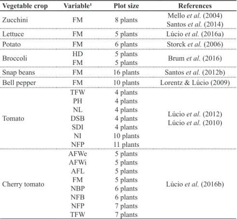
Plot size depends on the experimental material and objectives, number of treatments, seeds/seedlings availability, need for mechanization, total area, cost, time and labor available for implementing the experiment. Plot shape is also associated with experimental precision. In general, experimental precision increases with relatively long and narrow plots, since this shape allows for more plots in homogeneous conditions in the experimental area. Briefly, one can state that the most appropriate plot shape and size will be those that result in the least variation among plots of the same set. Plot size is estimated by uniformity tests, experiments without treatments and with homogeneous management. In vegetable crops, plot size has already been estimated for several species (Table 1). Therefore, when planning experiments, researchers must use this information, so that plot size in their experiments has technical-scientific basis.
The experimental material, i.e., any material employed in the experimental unit (pots, plants, seeds, substrates, etc.), must be carefully selected to be as homogeneous as possible. The experimental material should be related to the target population where conclusions and recommendations are drawn from. By using homogeneous experimental material, plots also tend to be more homogeneous, opening space
for using less complex experimental designs, such as the completely randomized design. The more basic the experimental design can be, the more degrees of freedom left for the experimental error and, consequently, the highest the experimental precision.
In experiments, we usually work with observation units, that is, the smallest part of the experimental material in which the observed variable is measured and recorded. It is common to researchers to evaluate only part of the experimental plot, called working area, or to perform samplings within the plot. There is a clear difference between these two approaches. When using the sample area, all individuals within the area are assessed and the value of the observed variable corresponds to the average of the values recorded individually. With the samplings, some individuals randomly and representatively taken are assessed, with the value of the
observed variable also being obtained by the average of the individual records. Besides these, a promising alternative is the covariance analysis, since there is interaction (border effect) between adjacent plants within the row. Santos
et al. (2014) showed that the use of
the mean of residues of two adjacent plots in the row as covariate (Papadakis method) reduces the experimental error, the optimal plot size and the minimum significant difference necessary to discriminate treatments in experiments with vegetables.
The use of sampling in plots adds a new source of variation (error) to experiments, defined as sample error. The sample error in the analysis of variance corresponds to the variability existing within the plot (since we are representing the plot by means of a sample), unlike the experimental error, which corresponds to the variability among plots. Generally speaking,
Table 1. Optimum plot size for different variables in vegetables. Santa Maria, UFSM, 2017. Vegetable crop Variable¹ Plot size References
Zucchini FM 8 plants Mello et al. (2004)
Santos et al. (2014)
Lettuce FM 5 plants Lúcio et al. (2016a)
Potato FM 6 plants Storck et al. (2006)
Broccoli HD
FM
5 plants
5 plants Brum et al. (2016)
Snap beans FM 16 plants Santos et al. (2012b)
Bell pepper FM 10 plants Lorentz & Lúcio (2009)
Tomato
TFW PH NL DSB
SDI NI NFP
4 plants 4 plants 4 plants 4 plants 4 plants 10 plants 11 plants
Lúcio et al. (2012) Lúcio et al. (2010)
Cherry tomato
AFWe AFWi AFL
FM NBP NFB NFP TFW
5 plants 5 plants 5 plants 5 plants 6 plants 6 plants 7 plants 7 plants
Lúcio et al. (2016b)
researchers neglect the sample error in the analysis of variance and do not consider it as an additional source of variation. Thus, the sample error ends up being added to the experimental error, inflating the MSE estimate. To circumvent it, the analysis of variance must consider experimental and sample errors as isolated sources of variation. Ideally, the sampling variation in the plot (sampling error) and among plots with the same treatment (experimental error) should be the same and the lowest possible. Thus, an experimental error with no significant effect indicates that sample variability within the plot and among plots of the same treatment is the same. When this effect is significant, the variability among plots is higher than the sample variability within the plot. Therefore, in addition to the plot size, the sample size should also be very well defined and described in the experimental plan, to prevent problems in collecting and, later, in the statistical analysis of the data. Fortunately, several studies on the adequate size of plot samples, for different vegetable crops, are available (Souza et al., 2002; Lúcio et al., 2003, 2012; Lorentz et al., 2004; Santos et al., 2010; Haesbaert et al.,
2011).
The characteristic assessed in the experimental unit that expresses the effect of the randomized treatment is called the observed variable, response variable or dependent variable. Such random variable can be random discrete or continuous and therefore must be very well determined and described in the experimental plan (What variable will be assessed? When? In which part of the EU - experimental unit – or of the individual the assessment will take place? Which equipment will be used? Which unit of measure will be used?). The definition of the random variable observed as random discrete or continuous when planning the experiment also informs researchers on the need to transform the experimental data, since, by definition of the statistical model, experimental errors should have a normal distribution of probability,
2
~ (0, ) ij
e N σ , which is read as: “all ɛij (i = 1,2, ..., I treatments, j = 1,2,
..., J replications) is identically and independently distributed in a normal way, with average zero and common variance σ2“.
The data collected in experiments, when meeting the assumptions of the statistical model, are prone to be analyzed, and the analysis of variance is the most frequent. Barbin (2003) elaborated in the relevance of knowing the nature of treatments, since treatments are the only controlled sources of variation, unlike others, such as the experimental error. This is another reason why the good choice and definition of treatments in the experimental plan is so important.
The number of treatments in an experiment should always be the minimum possible to meet the study’s objectives. If treatments are of fixed effect, the analysis of variance will estimate the individual effects of each one, comparing them to each other. If the treatments are of random effect, the analysis will estimate the components of variance, which are very important to plant breeding (Cochran & Cox, 1986; Pimentel Gomes, 1990; Barbin, 2003; Banzatto & Kronka, 2006; Storck et al., 2016).
Tests of Significance for a Group of Ranked Means are used to compare the estimates of treatments of fixed-effect when these treatments or factors have qualitative characteristics (shapes, features, methods, types, species, cultivars, etc.). On the other hand, Regression Analysis (RA) for different models is applied when treatments are quantitative (fertilizer or agrochemical doses, planting or sowing densities, evaluation time, etc.) (Cochran & Cox, 1986; Pimentel Gomes, 1990; Banzatto & Kronka, 2006; Storck et al., 2016).
According to Cardellino & Siewerdt (1992), these statistical procedures are often used indiscriminately, undermining the conclusions drawn from results, since information about intermediate treatments, such as economically significant contrasts and points of maximum technical and economic efficiency, are not produced.
Experiments can evaluate different numbers of factors. Experiments that evaluate single factors are denominated monofactorial and have their range of inference limited to uniform or constant conditions of all other controlled sources of variation. To increase the range of inference of an experiment, one can use factorial treatments, in which two or more factors, each one with two or more levels, are studied simultaneously. In this case, treatments consist of the combination of different levels of each factor and each factor can be of fixed or random effect.
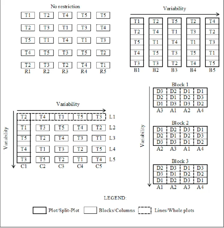
A particular case of factorial experiments is the split-plot design, in which the experiment has main plots in which one of the factors is randomized. Main plots are split in subplots, in which a second factor is randomized (Figure 1). Experiments in split-plot have two errors: one derived from the variation among main plots and, another, from the variation among subplots, which is the experimental error. These changes also impact the analysis of variance, more specifically on how to estimate the F test statistic.
analyze, interpret and present the results. Therefore, it is neither common, nor advisable to plan experiments with more than three factors.
Replication, Randomization and Local Control
To compare treatments and t o c o n c l u d e a b o u t t h e i r r e s u l t s
with known margin of confidence, every experiment should attend the following basic principles: Replication and Randomization (Zimmermann, 2004; Storck et al., 2016). The way
randomization is performed leads to a third principle, the Local Control (Pimentel Gomes, 1990; Banzatto & Kronka, 2006). Thus, there will only be a statistically valid experiment if
treatments are replicated and randomly distributed on the experimental units.
Replication refers to the application of the same treatment to two or more plots. The objective of replication is to confirm the individual’s response to a given treatment, to obtain an estimate of the experimental error (residual variance) and to obtain an estimate of the treatment average. Randomization,
Figure 1. Illustration of the completely randomized (upper left), complete blocks at random (upper right), Latin Square (lower left) and
in its turn, is the random assignment of treatments to the experimental plots, i.e., the distribution by chance of each treatment in each replication, contributing to the independence of residues.
Not only treatment assignment to plots, but also the order any cultural practice is carried out or any experimental evaluation is performed also requires randomization. Randomization objectives are to provide all treatments with the same probability of being assigned to any plot, to eliminate the involuntary tendency to protect a given treatment (s), to avoid treatments to be systematically favored or impaired in the replications and to build the independence of errors and other parameters of the statistical model. This is also one of the assumptions of the statistical model and guarantees that in the probabilistic interpretation of the experimental results, differences attributable to other factors do not bias the responses of applied different treatments.
The local control is how treatments are randomly assigned to the plots and prevents the variation among groups of plots from inflating the experimental error. The heterogeneous experimental area is divided into smaller and more homogeneous subareas, making the experimental design more efficient (Cochran & Cox, 1986; Pimentel Gomes, 1990; Banzatto & Kronka, 2006; Storck et al., 2016). Local control reduces the influence of the experimental area heterogeneity over the experimental precision.
The number of constraints to be used in treatment randomization is defined according to the sources of heterogeneity in the experimental area. In a homogeneous area, with truly homogeneous experimental units, there are no constraints to randomization and, thus, the completely randomized design is adopted. When the experimental area is heterogeneous due to a single source of variation, the experimental area is divided into homogeneous subareas, forming blocks of homogeneous experimental units, as in the design known as complete blocks at random. The only restriction of this design is
the need to randomize all treatments within each block. If the conditions of the experimental area are heterogeneous due to two sources of variation, then a double blocking of the experimental units is needed, and so the use of two restrictions when randomizing treatments. In these cases, the Latin Square design is used. In the Latin Square, treatments are randomized once inside each block that controls the first source of heterogeneity (line) and again inside each “block” that controls the second source of heterogeneity (column) (Figure 1).
In general, the higher the number of restrictions in the treatment randomization, the lower the number of degrees of freedom associated with the experimental error. Therefore, if restrictions are not efficient in reducing the variance of the experimental error, the experiment will lose efficiency due to the increase in the estimate of the mean square error. Therefore, local control should only be used when effectively needed.
The existing variability among planting rows is another issue that should be taken into consideration when planning experiments with vegetables. Variance heterogeneity among rows has two important consequences: the optimal plot size (the one that provides the lowest variance among plots) should be determined for each row and the experimental design should consider the variation among rows (Schwertner
et al., 2015 a,b). The plot size to be used
in the whole experiment is that estimated in the line of highest variability (Lúcio
et al., 2016b).
To confirm that the experiment is properly planned, researchers should answer “yes” to the following questions:
a) Is the experimental unit well defined and is it representative of the population inferences are meant to?;
b) Are the treatments under evaluation properly selected and do they reflect the purpose of the experiment?;
c) Is the process of assigning treatments to experimental plots designed in agreement with the heterogeneity of the experimental area?;
d) Does the number of replications
ensure adequate experimental accuracy? e) Are the descriptions of the observed variable clear and the process of measuring it understood?
f) All actions and activities inherent to implementation of the experiment are well defined and detailed?, and;
g) Is the statistical analysis of the experimental data being performed according to characteristics of the treatments and the experimental design?
Once these requirements are met, the experimental planning is complete. However, remember that there is always a probability of occurring heterogeneity among experimental plots, even in small parts of the area. Good judgment, good planning, and knowledge about the research object and the experimental material are fundamental in such cases. It is advisable to always try to reconcile variants, since drops in the experimental precision are inevitable. It is important to mitigate their effects and to be aware of where statistical problems are likely to arise and how severely they can interfere.
Implementing the experiment
Any process, action or activity carried out during experiment implementation should be performed as homogeneously as possible, so as not to inflate the experimental error. In addition, previous knowledge of existing specificities related to the management of vegetable crops should be taken into account already in the planning phase, as discussed earlier, to preserve the experimental precision.
sources of heterogeneity, which must be controlled, are introduced: labor force and the time required to carry out all crop practices. Whenever a crop practice involves a large number of people it becomes a great source of heterogeneity. Therefore, it is essential to level the team involved in the work to assure that crop management is carried out as homogeneously as possible throughout the experiment.
In addition, many practices cannot be completed on the same day due to the intensive management. In completely randomized designs, all activities must be finished on the same day (or less) and evenly carried out across all experimental plots, which requires training, efficiency and work team performance. In complete blocks at random or in the Latin square, crop practices can be carried out in one block and/or row at a time and not necessarily in all blocks and/or rows at the same day. If feasible, each block should be preferably managed and assessed by the same person. It contributes to the homogeneity within blocks and/ or rows. The heterogeneity that might arise among blocks and/or rows does not affect the experimental precision, since in these experimental designs its effects and variance are predicted in the model and evaluated separately.
Mechanized crop practices are generally more homogeneous than those carried out manually, provided that the equipment is properly calibrated and operators are well trained. The use of the same operator is an alternative to keep the procedure homogeneous, not forgetting fatigue as a possible source of variation.
Finally, manual harvesting is another important practice researchers should observe carefully. Any plant handling during the experiment can become a source of heterogeneity, especially in crops of multiple harvests. Training the harvesting team, especially to homogeneously recognize the harvesting point, may be fundamental for reducing the variability among harvests and plants. At harvest, the recommendation is the same as for crop management, each person should be responsible for harvesting a block and/or row in the case
of complete blocks at random block and Latin Square, and if possible, only one person should carry out the harvest in completely randomized designs.
Therefore, crop practices and harvests may become sources of heterogeneity that will significantly affect the experimental precision. To avoid it, researchers should train the work team; carry out crop practices in agreement with the experimental design; use plot sizes compatible with the crop and the variable; and describe clearly the harvesting point and the need for grouping harvests, as well as define the intervals between subsequent harvests.
The statistical analysis of the data
Once the planning and implementing phases are completed, then the statistical analysis of the experimental data comes to the spot. The procedure most commonly adopted by researchers is to perform the analysis of variance, followed by complementary tests (tests of significance for a group of ranked means or regression analysis) whenever significant differences among means are detected. However, some aspects must be observed, mainly in relation to the statistical assumptions, before carrying out the analysis of variance. These assumptions, regardless of the experimental design adopted, are:
- Additivity of the statistical model, i.e., parameters must be additive and independent;
- The ɛij are jointly independent, random, identically and normally distributed, with means equal to zero and common variance,εij~N
(
0; ²σ)
. All these assumptions are required for the hypothesis tests to be valid.The analysis of variance
In experiments with more than two means, the analysis of variance (ANOVA) is the procedure adopted to check if treatments are equal or not. Basically, ANOVA verifies, using the F test, if the variance among treatment effects is due or not to chance. F
calculated value corresponds to the ratio between the mean square of treatments, which represents the variance among treatment effects, and the means square error (MSE), which represents the random variation (variation inherent to any experiment + experimental error). It is thus understood that, if variation among treatments is due to chance, F value will be equal to 1. High calculated F values are an indication that the variation among treatments is greater than variations due to chance, so treatments do differ from each other. The
p-value can also be used as a decision
criterion. When p-value is lower than
the level of significance, the hypothesis H0 is rejected and it is concluded that treatments differ from each other.
When one carries out an analysis of variance, two questions should be answered: if the experimental design was efficient and if there is significant difference between the effects of treatments. The aspects related to reducing the variability in experiments with vegetables, previously discussed, have direct effect over the analysis of variance. Failures in experiment planning and implementation inflate the experimental error and, consequently, raise the value of the square mean error (SME). High SME values decrease the F-calculated value and make the differentiation between treatments more difficult, increasing the probability of accepting H0, even when it is false.
Residual analysis
be employed.
Here we present three graphical tools commonly used for residual analysis and their interpretations (Figure 2):
a) Frequency histogram: when values are concentrated at the graph edges, the distribution is not normal, but asymmetric. If the asymmetry is negative, values are concentrated to the right (Figure 2a); if the asymmetry is positive, values are concentrated to the left (Figure 2b). Kurtosis, on its turn, is related to curve flattening. The curve is called leptokurtic when it is “pointed” (Figure 2d), and platikurtic, when it is “flattened” (Figure 2e). Both conditions indicate that the distribution is not normal (Figure 2);
b) QQ-plot: when observed values assume an “arc” shape (Figures 2a and 2b) the distribution is asymmetric. When observed values are under the line, the distribution is normal, i.e., symmetrical and mesokurtic (Figure 2c). S-shaped values indicate that the curve is leptokurtic or platikurtic (Figures 2d and 2e);
c) Box-plot: when the box is displaced to the graph top, there is negative asymmetry (Figure 2a); if displaced to the graph bottom, the asymmetry is positive (Figure 2b); whilst when it is centralized, the distribution is normal (Figure 2c). Narrow boxes point to leptokurtic curves (Figure 2d), while long boxes indicate platikurtic curves (Figure 2e).
The statistical tests most commonly used to study the normality and homogeneity of experimental errors are:
a) Normality: Anderson Darling, Shapiro-Wilk, Kolmogorov-Smirnov;
b) Homogeneity: Bartlett and Levene. Bartlett test is used only when the assumption of normality of experimental errors is met.
Both ways of studying experimental e r r o r s h a v e a d v a n t a g e s a n d disadvantages. Graphical analysis tends to be more subjective, but it makes it possible to identify why assumptions are not met (asymmetry, outliers presence, kurtosis, mix of distributions). On the other hand, statistical tests are handier and less subjective, since the interpretation is based on the p-value:
the higher the p-value, the greater the
adherence to the normal distribution and the greater the experimental error homogeneity.
Meeting these assumptions is a basic condition for performing ANOVA and tests of significance for a group of ranked means (Barry, 1987). If the assumptions are not met, researchers can transform the data and carry out the diagnosis again. The most common data transformations are square root, logarithmic, Arcsin and Box-Cox (Yamamura, 1999; Couto
et al., 2009; Lúcio et al., 2011). If
even after transformation errors do not assume a normal distribution or become heterogeneous, then a non-parametric analysis must be used, such as Wilcoxon, Mann-Whitney-Wilcoxon, Friedman and Kruskal-Wallis (Conover, 1971; Campos, 1983).
The use of ANOVA is directly related to the assumption of normal distribution, homoscedasticity and independence of errors. Often these assumptions are violated because of heteroscedasticity, database inflation with zeros, and the very nature (distribution) of the variable (counting data, for example) (McCullagh & Nelder, 1989). In this sense, the use of generalized linear models (GLM) can be an alternative to ANOVA in experiments with vegetable crops. These models consist of a random component (which establishes the random variable distribution), a systematic component (which establishes the relation between the explanatory variables – factors – and the dependent variable) and a linking function that relates the systematic component to the random
component. An ANOVA statistical model is compared using the deviance analysis (ANODEV). In addition, in GLM mix models can be used to analyze the data (models inflated with zeros) (Zeileis et al., 2008; Zuur et al., 2009).
Complementary tests
When significant differences among treatments, with a given significance level, are detected, statistical tests are applied to complement the analysis of variance and discriminate the effects of treatments. The definition of which complementary statistical analysis will be applied depends on the nature of treatments: for qualitative treatments, tests of significance for a group of ranked means are used; for quantitative treatments, regression models. The most common complementary tests are:
a) tests of significance for a group of ranked means: t (LSD), Tukey, Duncan, Dunnett (two-way means comparison tests), Scheffé, orthogonal contrasts (tests for comparison among groups of means) and Scott & Knott (means clustering test).
b) Regression analysis: polynomial regression of Y (response variable) as function of X (levels of the quantitative treatment).
In factorial experiments, the complementary analysis should be carried out according to the ANOVA results. For significant interactions, factor levels must be statistically analyzed one within the other. When interactions are not significant, the average of the factors is used. The
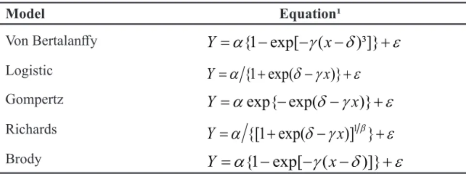
Table 2. Growth model examples. Santa Maria, UFSM, 2017.
Model Equation¹
Von Bertalanffy
Y
=
α
{1 exp[ (
−
−
γ
x
−
δ
)³]}
+
ε
Logistic Y=
α
{1 exp(+δ γ
− x)}+ε
Gompertz
Y
=
α
exp{ exp(
−
δ γ
−
x
)}
+
ε
Richards
{[1 exp(
)] }
1Y
=
α
+
δ γ
−
x
β+
ε
Brody
Y
=
α
{1 exp[ (
−
−
γ
x
−
δ
)]}
+
ε
¹ Y = dependent variable; x = independent variable; α = asymptote; γ = growth rate; δ = scale
E
D
Figure 2. Graphical representation of residues with negative asymmetry (A), positive asymmetry (B), normally distributed (C), leptokurtic
function (D) and platikurtic function (E). Santa Maria, UFSM, 2017.
C
A B
D group of ranked means to discriminate the levels of Factor D within each level of Factor A + tests of significance for a group of ranked means to discriminate the levels of Factor A within each level of Factor D;
ANOVA + tests of significance for a group of ranked means to discriminate levels of Factors A and D;
b) Factor A (qualitative) and Factor D (qualitative), significant interaction: ANOVA + tests of significance for a procedures to be adopted in a
two-factorial experiment for each of the possible situations are (Banzatto & Kronka, 2006; Storck et al., 2016):
c) Factor A (qualitative) and Factor D (quantitative), non-significant interaction: ANOVA + tests of significance for a group of ranked means to discriminate the levels of Factor A + regression adjustment for Factor D;
d) Factor A (qualitative) and Factor D (quantitative), significant interaction: ANOVA + tests of significance for a group of ranked means to discriminate the levels of Factor A within each level of Factor D + regression adjustment for Factor D within each level of Factor A;
e) Factor A (quantitative) and Factor D (quantitative), non-significant interaction: ANOVA + regression adjustment for Factors A and D;
f) Factor A (quantitative) and Factor D (quantitative), significant interaction: ANOVA + multiple regression adjustment with graphical representation by surface response.
Nonlinear regression
In multi-harvest vegetables, the adjustment of non-linear regression models is very interesting as an alternative to make inferences about production (Lúcio et al., 2015, 2016d,e).
As harvests accumulate, production grows exponentially at the beginning of the cycle, reach a point of maximum growth (inflection point) and, at the end, assume an asymptotic value (maximum production). These aspects can be quantified by means of parameters of the nonlinear models known as growth models (Table 2). Growth models have parameters with biological interpretation (
α
, which represents the asymptote andγ
, which represents the production rate), converting them into important tools to help describing the production behavior over time (Draper & Smith, 1981; Bates & Watts, 2007).The adjustment of growth models also requires the observation of some assumptions: error normality, homogeneity and independence. The diagnosis of error normality and homogeneity discussed previously can be thoroughly used in non-linear models. Regarding the error independence, the Durbin-Watson test, which checks the
presence of error autocorrelation, is the most commonly used. Tests to quantify the model nonlinearity must also be carried out, as they are important for verifying the quality of parameter adjustment. The lower the non-linearity, the higher the quality of the adjusted parameters (Draper & Smith, 1981; Bates & Watts, 2007).
Finally, unlike what was advised elsewhere, data transformation is not recommended in non-linear models, since it changes the value of the parameters, making them useless for biological interpretation. In case the assumptions of error homogeneity and independence are not met, two procedures are suggested: adjustment of the model by the weighted least square method, when the error variance is heterogeneous; and the generalized least square method, when errors are self-correlated (Draper & Smith, 1981; Bates & Watts, 2007).
Thus, the last step of an experiment, the analysis of the data, depends directly on the planning stage and is strongly influenced by how the experiment was implemented. With due planning and proper implementation of the experiment, the data collected will not be subject to large random variations, allowing for an adequate statistical analysis, consistent with the experiment purposes.
Reducing the variability in vegetable crops
The great variability influencing the growth of both plants and fruits, as well as the definition of maturity and of the harvest point, is caused by variations in environmental conditions, such as air temperature, total solar radiation, cloudiness and relative humidity. Vegetable crops are considerably affected by these. Regardless of the vegetable under evaluation, fruits do not appear simultaneously in different plants. On the contrary, as fruit setting depends on the development of new shoots throughout plant growth, fruit development is almost always uneven among plants. Thus, the occurrence of variance heterogeneity within each
harvest and between harvests is mainly due to the early or late maturation of some fruits, resulting from changes in the plant physiology or from adverse environmental conditions.
An option to identify data overdispersion and its causes may be to check the adjustment of the values obtained for the observed variables under multiple harvest conditions to the probability distribution these data possess, as well as the degree of independence among observations obtained on multiple consecutive harvests. This identification makes it possible to characterize the behavior of such databases, providing information on the most appropriate way to generate the values of the observed variables in the experimental plots, and thus avoiding problems inherent to overdispersion in the database. Another strategy, already mentioned here, is the accumulation of values of the production variables in each plant. The accumulation produces and increasing behavior in the values observed in the evaluated plants, thus enabling the use of regression analysis in the estimation of the variable values.
The definition of the ideal harvesting point in experiments with vegetables is still very subjective, as the harvest point is based on the size and/or color of the commercial plant part and varies according to each crop. In addition, some vegetables have the production staggered in the time, allowing for multiple harvests during its productive cycle.
Much work has already been carried out to develop strategies and to identify the most appropriate procedures so that data variability is minimized in experiments with vegetable crops. The most effective and also most used strategies to improve the quality of experiments with vegetables with multiple harvests are, namely, identification of crop-specific plot (Table 1) and sample sizes; determining the variability behavior between rows and between harvests, and; the study of data transformation and the use of Papadakis method to minimize the effects of excess zeros causing overdispersion in the database (Lúcio et al., 2011, 2016 a,c; Santos et al., 2012
a,b, 2014; Benz et al., 2015; Lúcio &
Benz, 2017).
Two procedures are efficient in reducing the variability in vegetables with multiple harvests: the clustering of harvests and plants. Studies in several vegetables have shown that harvest clustering reduces the variability between plants, decreasing data dispersion, and mitigating the negative effect of excess zeros in the database (Carpes et al.,
2008, 2010; Lúcio et al., 2011, 2016 b,
c; Santos et al., 2012 a,b, 2014; Benz et al., 2015; Lúcio & Benz, 2017).
However, even with harvest clustering, variability may go on increasing, as the cumulative value of harvest “n” remains the same as that observed in harvest “n-1”, when there are no products to be harvested in a plant, while in another, in which there are harvestable products, the value increases. This behavior is typical and common in vegetables with multiple harvests due to the uneven plant maturity and to the subjectivity of the harvest point.
A consequence of the high variability observed among plants when harvests are analyzed individually is the need of using larger plots, with several plants (Lorentz & Lúcio, 2009; Lúcio et al.,
2010, 2012, 2016 a,b; Santos et al.,
2012b, 2014). It results in underutilizing the experimental area, with likely reduction in the number of treatments and/or of experiments in the same area. It is emphasized that if researchers choose to use smaller plots, the experimental error increases and, consequently, the
experimental precision falls. High values for experimental errors lead to difficulty in detecting significant differences among treatments in the analysis of variance, poorer ability to discriminate treatments by means comparison tests (qualitative treatments) and reduced quality of regression adjustments (quantitative treatments).
Final remarks
To carry out experiments is an arduous task, which demands time, resources and labor to confirm or reject a previously defined hypothesis, drawn from the agricultural challenges in a given zone. Based on the statistical c o n c l u s i o n s o b t a i n e d a f t e r a l l stages of the experiment, practical recommendations, to be disseminated to farmers, are defined. Therefore, the experimentation process should be comprehensively carried out with the aim of best representing the population recommendations are meant to.
F o r c o n c l u s i o n s a n d recommendations to have high experimental precision and the highest degree of reliability, researchers must do their best to keep the residual variance (experimental error) as small as possible. To achieve this, experiments must be very well planned and implemented, targeting at homogeneity, so that the type II error rate is also the smallest possible. Knowledge about the experimental subject and material, as well as about experimentation techniques is fundamental, is key to success.
REFERENCES
BANZATTO, DA; KRONKA, SN. 2006. 4ed. Experimentação agrícola. Jaboticabal: FUNEP. 237p.
BARBIN, D. 2003. Planejamento e análise estatística de experimentos agronômicos. Arapongas: Midas. 194p.
BATES, DM; WATTS, DG. 2007. Nonlinear Regression Analysis and Its Applications. New York: John Wiley & Sons. 392p.
BENZ, V; LÚCIO, AD; LOPES, SJ. 2015. The spatial and temporal independence of Italian Zucchini production. Acta Scientiarum. Agronomy 37: 257-263.
BERRY, DA. 1987. Logarithmic transformations
in ANOVA. Biometrics 43: 439-456. BOX, GEP; COX, DR. 1964. An analysis of transformations. Journal of the Royal Society 26: 211–252.
BRUM, B; BRANDELERO, FD; VARGAS, TO; STORCK, L; ZANINI, PRG. 2016. Tamanho ótimo de parcela para avaliação da massa e diâmetro de cabeças de brócolis. Ciência Rural 46:447-463.
CAMPOS, H. 1983. Estatística experimental não-paramétrica. 4ed. Piracicaba: Departamento de Matemática e Estatística - ESALQ. 349p. CARDELLINO, RA; SIEWERDT, F. 1992.
Utilização adequada e inadequada dos testes de comparação de médias. Revista da Sociedade Brasileira de Zootecnia 21: 985-995. CARPES, RH; LÚCIO, AD; STORCK, L;
LOPES, SJ; ZANARDO, B; PALUDO, AL. 2008. Ausência de frutos colhidos e suas interferências na variabilidade da fitomassa de frutos de abobrinha italiana cultivada em diferentes sistemas de irrigação. Revista Ceres 55: 590-595.
COCHRAN, WG; COX, GM. 1986.Experimental design. 2ed. New York: John Wiley. 611p. CONOVER, WJ. 1971. Practical nonparametric
statistics. London: John Wiley. 462p. COUTO, MRM; LÚCIO, AD; LOPES, SJ;
CARPES, RH. 2009. Transformações de dados em experimentos com abobrinha italiana em ambiente protegido. Ciência Rural 39: 1701-1707.
DRAPER, N; SMITH, H. 1981. Applied regression analysis. 2ed. New York: John Wiley & Sons. 709p.
HAESBAERT, FM; SANTOS, D; LÚCIO, AD; BENZ, V; ANTONELLO, BI. 2011. Tamanho de amostra para experimentos com feijão-de-vagem em diferentes ambientes. Ciência Rural 41: 38-44.
LORENTZ, LH; LÚCIO, AD. 2009. Tamanho e forma de parcela para pimentão em estufa plástica. Ciência Rural 39: 2380-2387. LORENTZ, LH; LÚCIO, AD; BOLIGON, AA;
LOPES, SJ; STORCK, L. 2005. Variabilidade da produção de frutos de pimentão em estufa plástica. Ciência Rural 35: 316-323. LORENTZ, LH; LÚCIO, AD; STORCK, L;
LOPES, SJ; BOLIGON, AA; CARPES RH. 2004. Variação temporal do tamanho de amostra para experimentos em estufa plástica. Ciência Rural 34: 1043-1049.
LÚCIO, AD; BENZ, V. 2017. Accuracy in the estimates of zucchini production related to the plot size and number of harvests. Ciência Rural 47: e20160078.
LÚCIO, AD; SANTOS, D.; CARGNELUTTI FILHO, A.; SCHABARUM, DE. 2016a. Método de Papadakis e tamanho de parcela em experimentos com a cultura da alface. Horticultura Brasileira 34: 066-073. LÚCIO, AD; SARI, BG; PEZZINI, RV;
LIBERALESSO, V; DELATORRE, F; FAÉ, M. 2016b. Heterocedasticidade entre fileiras e colheitas de caracteres produtivos de tomate cereja e estimativa do tamanho de parcela. Horticultura Brasileira 34: 223-230. LÚCIO, AD; NUNES, LF; REGO, F; PASINI,
variables in trials with horticultural crops. Spanish Journal of Agricultural Research 14: 1-14.
LÚCIO, AD; SARI, BG; RODRIGUES, M; BEVILAQUA, LM; VOSS, HMG; COPETTI, D; FAÉ, M. 2016d. Modelos não-lineares para a estimativa da produção de tomate do tipo cereja. Ciência Rural 46: 233-241. LÚCIO, AD; NUNES, LF; REGO, F. 2016e.
Nonlinear regression and plot size to estimate green beans production. Horticultura Brasileira 34: 507-513.
LÚCIO, AD; NUNES, LF; REGO, F. 2015. Nonlinear models to describe production of
fruit in Cucurbita pepo and Capiscum annuum. Scientia Horticulturae 193: 286-293. LÚCIO, AD; HAESBAERT, FM; SANTOS,
D; SCHWERTNER, DV; BRUNES, RR. 2012. Tamanhos de amostra e de parcela para variáveis de crescimento e produtivas de tomateiro. Horticultura Brasileira 30: 660-668.
LÚCIO, AD; COUTO, MRM; LOPES, SJ; STORCK, L. 2011.Transformação box-cox em experimentos com pimentão em ambiente protegido. Horticultura Brasileira 29: 38 42. LÚCIO, AD; CARPES, RH; STORCK, L;
ZANARDO, B; TOEBE, M; PUHL, OJ; SANTOS, JRA. 2010. Agrupamento de colheitas de tomate e estimativas do tamanho de parcela em cultivo protegido. Horticultura Brasileira 28: 190-196.
LÚCIO, AD; CARPES, RH; STORCK, L; LOPES, SJ; LORENTZ, LH; PALUDO, AL. 2008. Variância e média da massa de frutos de abobrinha-italiana em múltiplas colheitas. Horticultura Brasileira 26: 335-341. LÚCIO, AD; LORENTZ, LH; BOLIGON,
AA; LOPES, SJ; STORCK, L; CARPES, RH. 2006. Variação temporal da produção de pimentão influenciada pela posição e características morfológicas das plantas em
ambiente protegido. Horticultura Brasileira 24: 31-35.
LÚCIO, AD; SOUZA, MF; HELDWEIN, AB; LIEBERKNECHT, D; CARPES, RH; CARVALHO, MP. 2003. Tamanho da amostra e método de amostragem para avaliação de características do pimentão em estufa plástica. Horticultura Brasileira 21: 180-184. McCULLAGH, P; NELDER, JA. 1989.
Generalized linear models. London: Chapman and Hall. 511 p.
MELLO, RM; LÚCIO, AD; STORCK, L; LORENTZ, LH; CARPES, RH; BOLIGON, AA. 2004. Size and form of plots for the culture of the Italian pumpkin in plastic greenhouse. Scientia Agricola 61: 457- 461. PIMENTEL GOMES, F. 1990. Curso de estatística
experimental. 13ed. Piracicaba: Nobel. 468p. SANTOS, D; LÚCIO, AD; STORCK,L;
CARGNELUTTI FILHO, A.; STORCK, L.; LORENTZ, LH; SCHABARUM, DE. 2014. Efeito de vizinhança e tamanho de parcela em experimentos com culturas olerícolas de múltiplas colheitas. Pesquisa Agropecuária Brasileira 49: 257-264.
SANTOS, D; HAESBAERT, FM; LÚCIO, AD; LOPES, SJ; CARGNELUTTI FILHO, A.; BENZ, V. 2012a. Aleatoriedade e variabilidade produtiva de feijão-de-vagem. Ciência Rural 42:1147-1154.
SANTOS, D; HAESBAERT, FM; LÚCIO, AD; STORCK, L; CARGNELUTTI FILHO, A. 2012b. Tamanho ótimo de parcela para a cultura do feijão-vagem. Revista Ciência Agronômica 43: 119-128.
SANTOS, D; HAESBAERT, FM; PUHL, OJ; SANTOS, JRA; LÚCIO, AD. 2010. Suficiência amostral para alface cultivada em diferentes ambientes. Ciência Rural 40: 800-805.
S C H W E RT N E R , D V; L Ú C I O , A D ;
CARGNELUTTI FILHO, A. 2015a. Size of uniformity trials for estimating the optimum plot size for vegetables. Horticultura Brasileira 33: 388-393.
S C H W E RT N E R , D V; L Ú C I O , A D ; CARGNELUTTI FILHO, A. 2015b. Uniformity trial size in estimates of plot size in restrict areas. Revista Ciência Agronômica 46: 597-606.
SOUZA, MF; LÚCIO, AD; STORCK, L; CARPES, RH; SANTOS, PM; SIQUEIRA, LF. 2002. Tamanho da amostra para peso da massa de frutos, na cultura da abóbora italiana em estufa plástica. Revista Brasileira de Agrociência 8: 123-128.
STEEL, RGD; TORRIE, JH; DICKEY, DA. 1997. Principles and procedures of statistics: a biometrical approach. 3ed. New York: McGraw-Hill. 666p.
STORCK, L; LOPES, SJ; ESTEFANEL, V; GARCIA, DC. 2016. Experimentação Vegetal.3Ed. Santa Maria: Editora UFSM. 198p.
STORCK, L; BISOGNIN, DA; OLIVEIRA, SJR. 2006. Dimensões dos ensaios e estimativas do tamanho ótimo de parcela em batata. Pesquisa Agropecuária Brasileira 41: 903-909. YAMAMURA, K. 1999. Transformation using (x
+ 0.5) to stabilize the variance of populations. Journal Researches on Population Ecology 42: 229–234.
ZEILEIS, A; KLEIBER, C; JACKMAN, S. 2008. Regression Models for Count Data in R. Journal of Statistical Software 27:1-25, 2008. ZIMMERMANN, FJP. 2004. Estatística aplicada à pesquisa agrícola. Santo Antônio de Goiás: Embrapa. 402p.