Three-way multivariate methods in the evaluation of patterns of stability and change in the eurozone countries

Texto

(1)UNIVERSITY OF THE ALGARVE FACULTY OF ECONOMICS. THREE-WAY MULTIVARIATE METHODS IN THE EVALUATION OF PATTERNS OF STABILITY AND CHANGE IN THE EUROZONE COUNTRIES Nelson Tavares da Silva THIS THESIS IS SUBMITTED IN PARTIAL FULFILMENT OF THE REQUIREMENTS FOR THE PHD IN QUANTITATIVE METHODS APPLIED TO ECONOMICS AND MANAGEMENT. Work elaborated under the supervision of: Professora Doutora Maria Purificación Galindo Villardón Universidad de Salamanca - Departamento de Estadística Professor Doutor Guilherme José Fresca Mirador de Andrade Castela Universidade do Algarve - Faculdade de Economia Professora Doutora Eugénia Maria Dores Maia Ferreira Castela Universidade do Algarve - Faculdade de Economia. Faro 2014.

(2) THREE-WAY MULTIVARIATE METHODS IN THE EVALUATION OF PATTERNS OF STABILITY AND CHANGE IN THE EUROZONE COUNTRIES. Statement of authorship. I hereby declare to be the author of this work, which is original and unpublished. Authors and studies reviewed are properly cited in the text and listed in the included bibliography listing.. Nelson Tavares da Silva. Copyright The University of Algarve has the perpetual right and without geographical boundaries, to archive and publicize this work through printed copies reproduced on paper or digital form, or by any other means known or to be invented, to release it through repositories scientific and admit their copying and distribution for educational purposes or for research, non-commercial, as long as credit is given to the author and editor.. ii.

(3) ACKNOWLEDGEMENTS. I would like to express my special appreciation and thanks to my supervisors Professor Guilherme Castela, Professor Eugénia Castela, and Professor Purificación Galindo, for supervising the research subjacent to this thesis and for having placed me challenges and helped me to achieve them. Your support and advices have been priceless. I would also like to thank my colleagues Ana Marreiros, Iris Lopes, João Vidal, and Daniela Patrício, for all their help and encouragement. A special thanks to my family. Words cannot express how grateful I am to my mother and father for all they’ve done for me. Angela, I thank you from the bottom of my heart for your patience in my absences and for your support during my presence.. iii.

(4) ABSTRACT In Multivariate Data Analysis it is usual to have several quantitative data tables, which are obtained in different occasions or conditions and standard two-way methods often fail to find the underlying structures in multiway arrays. With increasing number of application areas, multiway data analysis has become popular as an exploratory analysis tool, particularly in using methods such as STATIS (Structuration de Tableaux A Trois Indices de la Statistique) and MFA (Multiple Factor Analysis). The goal of these asymmetric methods is to compare multiple data tables, as well as investigate if there is a common structure between them. On the other hand, within the symmetrical methods, the TUCKER3 model is a three-mode method and permits a visualization of the structural relationships within three-way data tables, allowing a confirmatory analysis of the changes observed. They are similar according to the representation of individuals, variables, conditions and trajectories of individuals throughout conditions. The advantage of MFA compared to STATIS is that no group influences preponderantly the first axis of the compromise euclidean image allowing further interpretation of the axes. In turn, TUCKER3 has advantages over the MFA as the generation of additional trends and the measure of not only the relationships between components but also the interrelations among individuals, variables and conditions, which favor more interpretations. Nonetheless the STATIS and MFA vocation to study common data structures with the use of TUCKER3, by contrast, we intend to expand this information. However, the major aim of applying three-way data analysis is to reveal complex patterns of dependencies between the observations. In fact, the identification of benefits by the three methods is the feature which suggests consider them as complementary between themselves. This investigation intends to clarify the process that articulates growth with economic development in a context of comparable economies, and on a timeline that would not only allow evaluating periods of stability but also of change. In this sense, a set of disaggregated data on economic growth and development in twelve countries of the Eurozone, during the period 2005-2010 – the re-launch of the Lisbon Strategy – is analyzed. The aim is to describe and to compare the countries in their economic dynamics in periods of stability and change, during the three years prior to the 2008 economic and financial crisis and two years later. This theme outline led to the construction of three-dimensional data structures that require multivariate three-way analysis. This is done either in an exploratory perspective, where patterns among grouped variables to be measured from the observed variables are analyzed, or in a confirmatory aspect, starting from theoretical premises that confirm the degree of fit of observed data through constructs. The main findings of the research were that in the three methods there are countries that are similarly characterized and R&D is associated with economic growth. The STATIS method, only analyzed economic growth. Nonetheless it was still possible to analyze the main influences on economic growth as well the similarities in the type of growth in the twelve Eurozone countries. The MFA method distinguishes economic growth of economic development and includes the possibility of evaluating the twelve Eurozone countries, particularizing the role of development in the similarities and in the main influences of the economic identities. The TUCKER3 method examines with more detail the changes and influences of the economic identities, which become more realistic for the twelve Eurozone countries. TUCKER3 was able to identify the 2008 financial crisis, and the main interactions in the Eurozone, where the Benelux countries with Austria, Finland and Ireland revealed positive synergistic effects mostly on economic growth which also produced influence on economic development through Human Development Index (HDI) and, were negatively affected on Number of Patents (NP). The southern countries benefited from a positive synergistic effect from Germany and France on NP. On the other hand, they were negatively affected mostly on economic growth by the same two countries. These levels of dependency also influenced negatively the economic development through HDI. The three-way methods allowed not only to point out useful details for designing a more realistic economic and social diagnosis of the Eurozone for the period 2005-2010, but also to demonstrate the advantage of using information derived from the three-way methods, as a complement to the traditional methods of analysis. Keywords: Eurozone, economic growth, economic development, STATIS, MFA, TUCKER3. iv.

(5) RESUMO Embora na análise multivariada seja comum existirem várias tabelas de dados quantitativos, obtidas em diferentes ocasiões ou condições, os tradicionais métodos de duas vias não se revelam adequados para encontrar as estruturas comuns subjacentes. Com o crescente número de áreas de aplicação, a análise de dados de vias múltiplas tem-se tornado atrativa como ferramenta de análise exploratória, particularmente pela utilização de métodos como o STATIS (Structuration de Tableaux A Trois Indices de la Statistique) e a AFM (Análise Fatorial Múltipla). O objetivo destes métodos assimétricos é comparar várias tabelas de dados e investigar se existe uma estrutura comum entre elas. Embora semelhantes em termos da representação dos indivíduos, das variáveis, das condições e trajetórias de indivíduos através das várias condições, a AFM comparativamente ao STATIS tem a vantagem de nenhum grupo influenciar de forma preponderante o primeiro eixo da imagem euclidiana compromisso permitindo uma maior interpretabilidade dos eixos. Dentro dos métodos simétricos, o modelo TUCKER3 é um método de três modos que possibilita a visualização das relações estruturais dentro de quadros de dados de três vias, permitindo uma análise confirmatória das mudanças e das interações observadas. Por outro lado o método TUCKER3 apresenta algumas vantagens sobre a AFM como seja a geração de tendências e a medição não só das relações entre os eixos fatoriais, mas também das inter-relações entre indivíduos, variáveis e condições, o que possibilita mais interpretações. Não obstante a vocação dos métodos STATIS e AFM para o estudo de estruturas comuns, pretende-se aumentar essa informação por contraste com os resultados obtidos via TUCKER3. O principal objetivo de aplicar métodos para analisar dados de três vias é o de revelar padrões complexos de dependências entre as observações. Na verdade, a identificação dos benefícios de cada um dos três métodos sugerem considerá-los como complementares entre si. Efetivamente, um dos objetivos desta investigação é mostrar como os dados económicos podem ser interpretados a partir de uma matriz de dados multivariada complexa que, por sua vez, pode ser significativamente melhorada através da aplicação dos métodos de três vias. Deste modo, pretende-se clarificar o processo que articula o crescimento com desenvolvimento económico, num contexto de economias comparáveis, onde as dinâmicas económicas envolvem períodos de estabilidade e de mudança. Tradicionalmente, a análise económica faz uso de um conjunto de ferramentas estatísticas para reproduzir e simular os principais mecanismos de sistemas económicos regionais, nacionais ou internacionais. Assim, a fim de compreender a relação entre as variáveis económicas, aplicam-se modelos matemáticos para ajudar, em consonância com a teoria económica, o processo de tomada de decisão. A maioria destes modelos, que geralmente contêm variáveis macroeconómicas ou agregados, são designados por "econométricos" e, geralmente são definidos por estimações mediante uma variedade de métodos de cálculo. No entanto, a teoria macroeconómica não é um campo particularmente consensual de investigação, contendo muitas teorias diversas e conflituantes. Neste contexto, temas relacionados com o crescimento económico ou como o desenvolvimento económico podem, nalguns aspetos, ilustrar esta realidade. Questões quantitativas relativas ao Produto Interno Bruto, à Inovação e as questões sociais, tais como o Bem-Estar, o Índice de Desenvolvimento Humano e a Qualidade de Vida, entre outros, podem produzir interações que não são facilmente capturadas através dos modelos econométricos. De facto, o processo de desenvolvimento económico é geralmente associado à ideia de que uma variação positiva nas variáveis associadas ao crescimento é geralmente acompanhada de mudanças positivas em indicadores sociais como o Índice de Desenvolvimento Humano, resultando em melhoria dos padrões de vida. Porém, isto nem sempre se materializa. A ocorrência destes factos representa, em nossa opinião, uma oportunidade para a utilização de ferramentas de estatística multivariada, tais como os modelos de três-vias, para promover outras abordagens. Na verdade, tem havido pouca convergência científica para ultrapassar as barreiras operacionais e estas abordagens podem contribuir significativamente para melhorar a compreensão das ligações entre várias metodologias de análise. Esta falta de complementaridade deve-se principalmente às diferentes origens disciplinares dos investigadores, aos diferentes métodos utilizados e, no seio da análise multivariada de três-vias, às dificuldades de compatibilidade nalguns dos conceitos utilizados pelas escolas francesa e anglo-saxónica. Este trabalho também representa uma tentativa de reduzir esta lacuna na investigação através da combinação dos três métodos de três-vias, dois da escola. v.

(6) francesa e um da escola anglo-saxónica. O objetivo não é apresentar uma equivalência matemática ou uma notação similar entre as técnicas, mas sim evidenciar a complementaridade da interpretação dos três métodos a qual pode revelar-se extremamente útil para apoiar outras técnicas de análise. Assim, o recurso a um conjunto de dados desagregados sobre os países da Zona Euro, durante o período 2005-2010, coincidente com o relançamento da estratégia de Lisboa, possibilitou a construção de estruturas tridimensionais de dados propícios a uma análise multivariada de três-vias. Seja numa perspetiva exploratória, onde padrões entre condições económicas são analisados ou, num contexto confirmatório mediante premissas teóricas que confirmam a confiança dos dados observados, os métodos propostos possibilitam, em nosso entender, não apenas detalhar a realidade económica e social da Zona Euro, como também destacar informação útil ao processo de decisão em matéria de política económica europeia. As principais conclusões são de que nos três métodos existem países caracterizados de forma similar e que o investimento em Investigação e Desenvolvimento está associado ao crescimento económico. (i) O método STATIS analisa somente o crescimento económico. No entanto foi possível analisar as principais influências no crescimento económico bem como as similaridades no tipo de crescimento para os doze países da Zona Euro. (ii) A AFM distinguiu crescimento económico de desenvolvimento económico e incluiu a possibilidade de avaliá-los para os doze países da Zona Euro, particularizando o papel do desenvolvimento nas similaridades e principais influências das entidades económicas. (iii)O método TUCKER3 analisou com maior detalhe as mudanças e as influências das entidades económicas, que se tornam mais realistas para os doze países da Zona Euro. Com este método foi possível identificar a crise financeira de 2008, e as principais interações da Zona Euro, onde os países Benelux associados com a Áustria, Finlândia e Irlanda revelaram efeitos sinergéticos positivos, predominantemente no crescimento económico, que produziram influências no desenvolvimento económico através do Índice de Desenvolvimento Humano (HDI) e, por outro lado, foram afetados negativamente no Número de Patentes (NP). Os países do sul sofreram um efeito sinergético positivo da Alemanha e França no NP. No entanto foram afetados negativamente, essencialmente no crescimento económico, pelos mesmos dois países. Estes níveis de dependência influenciaram também negativamente o desenvolvimento económico através do HDI. Pensamos que um diagnóstico socioeconómico mais pormenorizado da Zona Euro para o período em causa, resultante da informação dos métodos de três-vias, será vantajoso, sobretudo como complemento aos métodos tradicionais de análise económica. Esta abordagem metodológica descreve, compara e analisa 12 países no que concerne às suas dinâmicas de crescimento e de desenvolvimento durante os 3 anos anteriores à crise económico-financeira de 2008 e nos 2 anos seguintes, recriando assim cenários de estabilidade e de mudança na Zona Euro.. Palavras-chave: zona euro, crescimento económico, desenvolvimento económico, STATIS, AFM, TUCKER3. vi.

(7) GENERAL INDEX AKNOWLEDGMENTS…….…….…………………………….………...…………………...……………iii ABSTRACT………………………………………………………………………...…………....……...…..iv RESUME…………………….…………….…………………………………………………………………v GENERAL INDEX………….……………………………………………………………...………………vii FIGURE INDEX……………..……………….………………………………………………………...…....x TABLE INDEX………………………………………………………………………………...........……..xiii LIST OF ABBREVIATIONS....……………………………………………….....……………………....…xv. 1. CHAPTER 1 – INTRODUCTION ............................................................................................. 1 1.1 Overview ................................................................................................................................. 2 1.2 The Eurozone .......................................................................................................................... 5 1.3 Technology and innovation as drivers for economic growth ................................................. 6 1.4 The 2008 global crisis as a turning point of stability and change ........................................... 9 1.5 Challenges for economic growth and development of the EU ............................................. 11 1.6 Problematic of mechanisms and methods for economic development and growth analysis 12 1.7 A three-way multivariate approach ....................................................................................... 14 1.8 The aims of the research ....................................................................................................... 16 1.9 The relevance of the research ............................................................................................... 18 1.10 The research structure .......................................................................................................... 19. 2. CHAPTER 2 – LITERATURE REVIEW ................................................................................ 20 2.1 Introduction ........................................................................................................................... 21 2.2 The European Union context with focus on the Eurozone ................................................... 22 2.3 Discrepancies of economic growth and development on the EU ......................................... 27 2.4 The influence of the 2008 global crisis on stability and change in Eurozone countries ....... 33 2.5 Economic Growth, Patents, Research and Development and Human Development ........... 37 2.5.1 Gross Domestic Product as a measure of Economic Growth .......................................... 39 2.5.2 R&D expenditure as a measure of countries’ research and development intensity ........ 41 2.5.3 Patents as a measure for knowledge transfer to technology ............................................ 42 2.5.4 HDI as a measure of human development achievements ................................................ 44 2.6 Traditional methods for economic development and growth analysis ................................. 45 2.7 The three-way tables and techniques .................................................................................... 50 2.7.1 Asymmetric methods ....................................................................................................... 53 2.7.1.1 STATIS ..................................................................................................................... 54 2.7.1.2 Multiple factor analysis ............................................................................................ 55 2.7.2 Symmetric methods ......................................................................................................... 56 2.7.2.1 TUCKER3 ................................................................................................................ 57 vii.

(8) 2.7.2.2 PARAFAC and CANDECOMP ............................................................................... 58 2.7.3 Comparison of Methods .................................................................................................. 58 3. CHAPTER 3 – METHODOLOGY .......................................................................................... 60 3.1 Introduction ........................................................................................................................... 61 3.2 Principal Component Analysis ............................................................................................. 61 3.2.1 Main features ................................................................................................................... 61 3.2.2 Individuals ....................................................................................................................... 64 3.2.3 Variables .......................................................................................................................... 68 3.2.4 Projection of individuals in a subspace ........................................................................... 70 3.2.5 Projection of the variables in a subspace ......................................................................... 76 3.2.6 Duality and transition relations ....................................................................................... 78 3.2.7 Quality and interpretation of results ................................................................................ 81 3.2.7.1 Reconstitution formulas ............................................................................................ 81 3.2.7.2 Quality measures....................................................................................................... 83 3.2.7.3 Circle of correlations ................................................................................................ 87 3.2.7.4 Number of axes to consider ...................................................................................... 89 3.3 STATIS ................................................................................................................................. 90 3.3.1 The procedure .................................................................................................................. 91 3.3.2 The interstructure............................................................................................................. 92 3.3.3 The compromise .............................................................................................................. 97 3.3.4 The intrastructure........................................................................................................... 102 3.4 MFA ................................................................................................................................. 105 3.4.1 The intrastructure........................................................................................................... 106 3.4.2 Representation of Individuals ........................................................................................ 107 3.4.3 Simultaneous representation of the T clouds................................................................. 108 3.4.4 Representation of variables ........................................................................................... 110 3.4.5 The interstructure........................................................................................................... 111 3.4.5.1 Representation of groups of variables .................................................................... 111 3.4.5.2 Interpretation of the scalar product between two groups ........................................ 112 3.5 TUCKER3 .......................................................................................................................... 118 3.5.1 Unfolding the original data array .................................................................................. 118 3.5.2 Data preprocessing ........................................................................................................ 122 3.5.3 Estimation of model parameters .................................................................................... 124 3.5.4 Analysis of model fit ..................................................................................................... 126 3.5.4.1 Timmerman-Kiers DifFit procedure ....................................................................... 126 3.5.4.2 Deviance analysis ................................................................................................... 128 3.5.4.3 Ceulemans-Kiers st-criterion or numerical convex-hull ......................................... 129 viii.

(9) 3.5.5 Representation and interpretation of the solution .......................................................... 131 3.6 Comparison of methods ...................................................................................................... 132 4. CHAPTER 4 – RESULTS...................................................................................................... 135 4.1 Methodological procedure .................................................................................................. 136 4.2 Data Description ................................................................................................................. 137 4.3 Preliminary analysis of the data .......................................................................................... 137 4.4 Preprocessing and construction of three-way data structures ............................................. 142 4.5 Application of three-way methods: STATIS, MFA and TUCKER3 .................................. 157 4.5.1 The 12 countries of the Eurozone from a three-way analysis perspective .................... 158 4.5.2 The period 2005-2010 from a three-way analysis point of view................................... 164 4.5.3 A three-way analysis of growth and economic development ........................................ 170 4.5.4 Trends of the 12 countries of the Eurozone................................................................... 175 4.5.5 2005-2010 interactions in Eurozone countries .............................................................. 225 4.6 Discussion ........................................................................................................................... 238 4.6.1 Economic growth and development in the Eurozone .................................................... 238 4.6.2 Stability and change effects on trends over 2005-2010................................................. 242 4.6.3 2005-2010 interactions in Eurozone countries .............................................................. 246 4.6.4 A comparison between the results of STATIS, MFA, and TUCKER3......................... 248. 5. CHAPTER 5 – CONCLUSIONS, LIMITATIONS AND SUGGESTIONS FOR FURTHER RESEARCH ........................................................................................................................... 250 5.1 Conclusions ......................................................................................................................... 251 5.1.1 In the context of economic growth and development in the Eurozone ......................... 251 5.1.2 A perspective of stability and change over 2005-2010 and its effects on the countries’ trends .......................................................................................................................... 252 5.1.3 2005-2010 main interactions in Eurozone countries ..................................................... 253 5.1.4 Relevance in the use of the three-way methods ............................................................ 254 5.2 Research limitations ............................................................................................................ 255 5.3 Suggestions for further research ......................................................................................... 255. BIBLIOGRAPHIC REFERENCES .............................................................................................. 256 6. APPENDIX ............................................................................................................................ 274. ix.

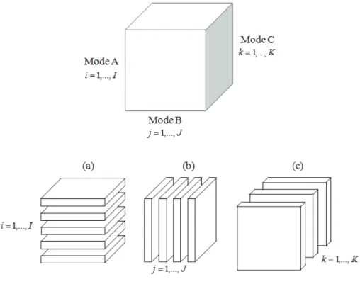
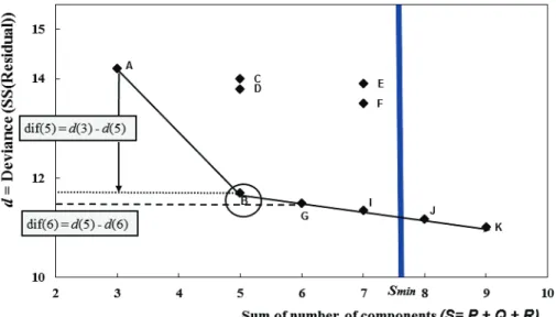
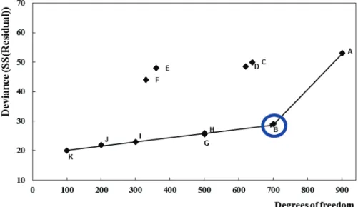
(10) FIGURE INDEX Figure 2.1 – R&D expenditure % of GDP per country 2005-2009 ....................................................................... 31 Figure 2.2 – HDI Dimensions ............................................................................................................................... 45 Figure 3.1 – Cloud of individuals in F space ......................................................................................................... 64 Figure 3.2 – Cloud of variables in space E ............................................................................................................ 69 Figure 3.3 – Projection of the individual xi on the uk axis ..................................................................................... 70 Figure 3.4 – Projection of xk in vk axis .................................................................................................................. 77 Figure 3.5 – Duality relations between principal axes and principal components ................................................. 79 Figure 3.6 – Duality scheme of PCA ..................................................................................................................... 80 Figure 3.7 – Projection of the individual xi in the uk,ul plane ............................................................................... 84 Figure 3.8 – Projection of the variable xj in the vk,vl plane ................................................................................... 85 Figure 3.9 – Coordinates of the variable xj in the correlations circle .................................................................... 88 Figure 3.10 –Correlations circle interpretation ...................................................................................................... 88 Figure 3.11 – Scree plot......................................................................................................................................... 89 Figure 3.12 – T data tables .................................................................................................................................... 91 Figure 3.13 – Representation of objects in the main plane .................................................................................... 96 Figure 3.14 – Representation and interpretation of objects in the main plane ....................................................... 99 Figure 3.15 – Juxtaposition of the STATIS tables............................................................................................... 101 Figure 3.16 – Table of data ܺത t ............................................................................................................................. 107 మ Figure 3.17 – Representation of variable groups in Թ௡ and Թ௡ ......................................................................... 115 Figure 3.18 – Three-way array, cut into (a) horizontal, (b) lateral, and (c) frontal slices .................................... 119 Figure 3.19 – Three-way array, cut into (a) horizontal, (b) vertical and (c) depth fibers .................................... 122 Figure 3.20 – Multiway scree plot: Deviance versus sum of components .......................................................... 127 Figure 3.21 – Deviance plot: Deviance versus degrees of freedom..................................................................... 128 Figure 3.22 – Celeumans-Kiers heuristic for selecting a model in the deviance plot .......................................... 131 Figure 3.22 – Decision diagram for STATIS, MFA and TUCKER3 .................................................................. 134 Figure 4.1 – Methodological procedure............................................................................................................... 136 Figure 4.2 – Profile comparison of GDP per capita, R&D expenditure, NP, and HDI ....................................... 138 Figure 4.3 – Construction of three-way data structure ........................................................................................ 143 Figure 4.4 – Construction of the initial array for STATIS .................................................................................. 143 Figure 4.5 – Construction of the concatenated supermatrix for MFA ................................................................. 144 Figure 4.6 – TUCKER3: Mode A (12x48 matrix)............................................................................................... 144 Figure 4.7 – TUCKER3: Mode B (6x96 matrix) ................................................................................................. 144 Figure 4.8 – TUCKER3: Mode C (8x72 matrix) ................................................................................................. 145 Figure 4.9 – Three-mode deviance plot ............................................................................................................... 149 Figure 4.10 – Three-mode scree plot ................................................................................................................... 150 Figure 4.11 – PCA representation for Mode A – axes 1-2, 1-3 and 2-3 .............................................................. 153 Figure 4.12 – PCA representation for Mode B – axes 1-2 .................................................................................. 155 Figure 4.13 – PCA representation for Mode C – axes 1-2, 1-3 and 2-3 .............................................................. 156 Figure 4.14 – Results presentation structure........................................................................................................ 157 Figure 4.15 – Comparison of STATIS Compromise, MFA Consensus with TUCKER3 Mode A ..................... 162 Figure 4.16 – Correlation circles: a comparison of STATIS, MFA and TUCKER3 (Mode A) .......................... 168 Figure 4.17 – Comparison of STATIS and MFA Interstructures with TUCKER3 Mode C ............................... 173 Figure 4.18 – Comparison of STATIS and MFA: Projection of economic growth and development on Luxembourg’s factorial representation ................................................................................................................ 177 Figure 4.19 –TUCKER3 Mode C and Mode B: Projection of economic growth and development on Luxembourg’s factorial representation ................................................................................................................ 179 Figure 4.20 – Comparison of STATIS and MFA: Projection of economic growth and development on Ireland’s factorial representation ........................................................................................................................................ 181. x.

(11) Figure 4.21 –TUCKER3 Mode C and Mode B: Projection of economic growth and development on Ireland’s factorial representation ........................................................................................................................................ 183 Figure 4.22 – Comparison of STATIS and MFA: Projection of economic growth and development on the Netherlands’ factorial representation ................................................................................................................... 185 Figure 4.23 – TUCKER3 Mode C and Mode B: Projection of economic growth and development on the Netherlands’ factorial representation ................................................................................................................... 187 Figure 4.24 – Comparison of STATIS and MFA: Projection of economic growth and development on Finland’s factorial representation ........................................................................................................................................ 189 Figure 4.25 – TUCKER3 Mode C and Mode B: Projection of economic growth and development on Finland’s factorial representation ........................................................................................................................................ 191 Figure 4.26 – Comparison of STATIS and MFA: Projection of economic growth and development on Austria’s factorial representation ........................................................................................................................................ 193 Figure 4.27 – TUCKER3 Mode C and Mode B: Projection of economic growth and development on Austria’s factorial representation ........................................................................................................................................ 195 Figure 4.28 – Comparison of STATIS and MFA: Projection of economic growth and development on Belgian’s factorial representation ........................................................................................................................................ 197 Figure 4.29 – TUCKER3 Mode C and Mode B: Projection of economic growth and development on Belgian’s factorial representation ........................................................................................................................................ 199 Figure 4.30 – Comparison of STATIS and MFA: Projection of economic growth and development on Germany’s factorial representation ........................................................................................................................................ 201 Figure 4.31 – TUCKER3 Mode C and Mode B: Projection of economic growth and development on Germany’s factorial representation ........................................................................................................................................ 203 Figure 4.32 – Comparison of STATIS and MFA: Projection of economic growth and development on France’s factorial representation ........................................................................................................................................ 205 Figure 4.33 – TUCKER3 Mode C and Mode B: Projection of economic growth and development on France’s factorial representation ........................................................................................................................................ 207 Figure 4.34 – Comparison of STATIS and MFA: Projection of economic growth and development on Italy’s factorial representation ........................................................................................................................................ 209 Figure 4.35 – TUCKER3 Mode C and Mode B: Projection of economic growth and development on Italy’s factorial representation ........................................................................................................................................ 211 Figure 4.36 – Comparison of STATIS and MFA: Projection of economic growth and development on Spain’s factorial representation ........................................................................................................................................ 213 Figure 4.37 – TUCKER3 Mode C and Mode B: Projection of economic growth and development on Spain’s factorial representation ........................................................................................................................................ 215 Figure 4.38 – Comparison of STATIS and MFA: Projection of economic growth and development on Greece’s factorial representation ........................................................................................................................................ 217 Figure 4.39 – TUCKER3 Mode C and Mode B: Projection of economic growth and development on Greece’s factorial representation ........................................................................................................................................ 219 Figure 4.40 – Comparison of STATIS and MFA: Projection of economic growth and development on Portugal’s factorial representation ........................................................................................................................................ 221 Figure 4.41 – TUCKER3 Mode C and Mode B: Projection of economic growth and development on Portugal’s factorial representation ........................................................................................................................................ 223 Figure 4.42 – TUCKER3 Mode A axes 1-2 for the 1st element of the Core matrix ........................................... 226 Figure 4.43 – TUCKER3 Mode B axes 1-2 for the 1st element of the Core matrix............................................ 227 Figure 4.44 – TUCKER3 Mode C axes 1-2 for the 1st element of the Core matrix............................................ 227 Figure 4.45 – BIPLOT: countries and economic conditions in the 1st element of the Core matrix .................... 229 Figure 4.46 – TUCKER3 Mode A axes 2-3 for the 2nd element of the Core matrix .......................................... 230 Figure 4.47 – TUCKER3 Mode B axes 1-2 for the 2nd element of the Core matrix .......................................... 231 Figure 4.48 – TUCKER3 Mode C axes 2-3 for the 2nd element of the Core matrix .......................................... 231 Figure 4.49 – BIPLOT: countries and economic conditions in the 2nd element of the Core matrix ................... 233 Figure 4.50 – TUCKER3 Mode A axes 1-3 for the 3rd element of the Core matrix ........................................... 234 Figure 4.51 – TUCKER3 Mode B axes 1-2 for the 3rd element of the Core matrix ........................................... 235 Figure 4.52 – TUCKER3 Mode C axes 1-3 for the 3rd element of the Core matrix ........................................... 235. xi.

(12) Figure 4.53 – BIPLOT: countries and economic conditions in the 3rd element of the Core matrix ................... 237 Figure 4.54 – STATIS: interstructure, compromise and original variables correlation ....................................... 238 Figure 4.55 – MFA: interstructure, consensus and original variables correlation ............................................... 239 Figure 4.56 – TUCKER3: Mode C and original variables correlation with Mode A .......................................... 240. xii.

(13) TABLE INDEX Table 2.1 – Eurozone member states by date of admission until December 31st 2014 ......................................... 26 Table 2.2 – Research and development expenditure (% of GDP) ......................................................................... 30 Table 2.3 – Literature review of innovation and economic growth related studies ............................................... 49 Table 4.1 – Identification of economic growth and development entities ........................................................... 137 Table 4.2 – Evolution of GDP ............................................................................................................................. 139 Table 4.3 – Patterns of GDP ................................................................................................................................ 139 Table 4.4 – Evolution of R&D ............................................................................................................................ 140 Table 4.5 – Patterns of R&D ............................................................................................................................... 140 Table 4.6 – Evolution of NP ................................................................................................................................ 140 Table 4.7 – Patterns of NP ................................................................................................................................... 141 Table 4.8 – Evolution of HDI .............................................................................................................................. 141 Table 4.9 – Patterns of HDI evolution ................................................................................................................. 142 Table 4.10 – TUCKER3: Mode A components................................................................................................... 145 Table 4.11 – TUCKER3: Mode A singular values and inertia ............................................................................ 145 Table 4.12 – TUCKER3: Mode B components ................................................................................................... 146 Table 4.13 – TUCKER3: Mode B singular values and inertia ............................................................................ 146 Table 4.14 – TUCKER3: Mode C components ................................................................................................... 147 Table 4.15 – TUCKER3: Mode C singular values and inertia ............................................................................ 147 Table 4.16 – Results of the relevant models ........................................................................................................ 148 Table 4.17 – TUCKER3: Summary of the three models selected by each dimensionality test ........................... 150 Table 4.18 – TUCKER3: Optimal core matrix .................................................................................................... 151 Table 4.19 – TUCKER3: Mode A components ................................................................................................... 152 Table 4.20 – TUCKER3: Mode A singular values and inertia ............................................................................ 152 Table 4.21 – TUCKER3: Mode B components ................................................................................................... 154 Table 4.22 – TUCKER3: Mode B singular values and inertia ............................................................................ 154 Table 4.23 – TUCKER3: Mode C components ................................................................................................... 155 Table 4.24 – TUCKER3: Mode C singular values and inertia ............................................................................ 155 Table 4.25 – STATIS: Euclidian image of the compromise space in axes 1-2 ................................................... 158 Table 4.26 – STATIS: Compromise space singular values and inertia ............................................................... 158 Table 4.27 – MFA: Euclidian image of the consensus space in axes 1-2 ............................................................ 159 Table 4.28 – MFA: Consensus space singular values and inertia ........................................................................ 159 Table 4.29 – TUCKER3: Euclidian image of Mode A in axes 1-2 ..................................................................... 160 Table 4.30 – TUCKER3: Mode A singular values and inertia ............................................................................ 160 Table 4.31 – Performance similarities of the countries in axes 1-2 ..................................................................... 164 Table 4.32 – STATIS: Correlation of the original variables with axis 1 of compromise space .......................... 165 Table 4.33 – STATIS: Correlation of the original variables with axis 2 of compromise space .......................... 165 Table 4.34 – MFA: Correlation of the original variables with axis 1 of consensus space ................................... 165 Table 4.35 – MFA: Correlation of the original variables with axis 2 of consensus space ................................... 166 Table 4.36 – TUCKER3 – MODE A: Correlation of the original variables with axis 1 of Mode A ................... 166 Table 4.37 – TUCKER3 – MODE A: Correlation of the original variables with axis 2 of Mode A ................... 166 Table 4.38 – Performance similarities of 2005-2010 over growth and development in axes 1-2........................ 169 Table 4.39 – STATIS: Interstructure Euclidian image coordinates in axes 1-2 .................................................. 170 Table 4.40 – STATIS: Interstructure singular values and inertia ........................................................................ 170 Table 4.41 – MFA: Interstructure Euclidian image coordinates in axes 1-2 ....................................................... 171 Table 4.42 – MFA: Interstructure singular values and inertia ............................................................................. 171 Table 4.43 – TUCKER3: Mode C Euclidian image coordinates in axes 1-2 ...................................................... 172 Table 4.44 – TUCKER3: Mode C singular values and inertia ............................................................................ 172 Table 4.45 – Performance similarities of growth and development over 2005-2010 in axes 1-2........................ 175 Table 4.46 – Compromise/consensus coordinates of economic growth and development for Luxembourg ....... 176 Table 4.47 – Luxembourg’s Performance from STATIS and MFA point of view.............................................. 178. xiii.

(14) Table 4.48 – Luxembourg’s Performance from TUCKER3 point of view ......................................................... 180 Table 4.49 – Compromise/consensus coordinates of economic growth and development for Ireland ................ 180 Table 4.50 – Ireland’s Performance from STATIS and MFA point of view ....................................................... 182 Table 4.51 – Ireland’s Performance from TUCKER3 point of view ................................................................... 184 Table 4.52 – Compromise/consensus coordinates of economic growth and development for the Netherlands .. 184 Table 4.53 – The Netherland’s Performance from STATIS and MFA point of view ......................................... 186 Table 4.54 – The Netherland’s Performance from TUCKER3 point of view ..................................................... 188 Table 4.55 – Compromise/consensus coordinates of economic growth and development for Finland ............... 188 Table 4.56 – Finland’s Performance from STATIS and MFA point of view ...................................................... 190 Table 4.57 – Finland’s Performance from TUCKER3 point of view .................................................................. 192 Table 4.58 – Compromise/consensus coordinates of economic growth and development for Austria ............... 192 Table 4.59 – Austria’s Performance from STATIS and MFA point of view ...................................................... 194 Table 4.60 – Austria’s Performance from TUCKER3 point of view .................................................................. 196 Table 4.61 – Compromise/consensus coordinates of economic growth and development for Belgium ............. 196 Table 4.62 – Belgium Performance from STATIS and MFA point of view ....................................................... 198 Table 4.63 – Belgium Performance from TUCKER3 point of view ................................................................... 200 Table 4.64 – Compromise/consensus coordinates of economic growth and development for Germany ............ 200 Table 4.65 – Germany’s Performance from STATIS and MFA point of view ................................................... 202 Table 4.66 – Germany’s Performance from TUCKER3 point of view ............................................................... 204 Table 4.67 – Compromise/consensus coordinates of economic growth and development for France ................ 204 Table 4.68 – France’s Performance from STATIS and MFA point of view ....................................................... 206 Table 4.69 – France’s Performance from TUCKER3 point of view ................................................................... 208 Table 4.70 – Compromise/consensus coordinates of economic growth and development for Italy .................... 208 Table 4.71 – Italy’s Performance from STATIS and MFA point of view ........................................................... 210 Table 4.72 – Italy’s Performance from TUCKER3 point of view ....................................................................... 212 Table 4.73 – Compromise/consensus coordinates of economic growth and development for Spain .................. 212 Table 4.74 – Spain’s Performance from STATIS and MFA point of view ......................................................... 214 Table 4.75 – Spain’s Performance from TUCKER3 point of view ..................................................................... 216 Table 4.76 – Compromise/consensus coordinates of economic growth and development for Greece ................ 216 Table 4.77 – Greece’s Performance from STATIS and MFA point of view ....................................................... 218 Table 4.78 – Greece’s Performance from TUCKER3 point of view ................................................................... 220 Table 4.79 – Compromise/consensus coordinates of economic growth and development for Portugal .............. 220 Table 4.80 – Portugal Performance from STATIS and MFA point of view........................................................ 222 Table 4.81 – Portugal Performance from TUCKER3 point of view ................................................................... 224 Table 4.82 – Signs of countries for the 1st element of the Core matrix .............................................................. 226 Table 4.83 – Signs of years for the 1st element of the Core matrix .................................................................... 227 Table 4.84 – Signs of economic conditions for the 1st element of the Core matrix ............................................ 228 Table 4.85 – Interaction results for the 1st element of the Core matrix .............................................................. 228 Table 4.86 – Signs of countries for the 2nd element of the Core matrix ............................................................. 230 Table 4.87 – Signs of years for the 2nd element of the Core matrix ................................................................... 231 Table 4.88 – Signs of the economic conditions for the 2nd element of the Core matrix ..................................... 232 Table 4.89 – Interaction results for the 2nd element of the Core matrix ............................................................. 232 Table 4.90 – Signs of the countries for the 3rd element of the Core matrix ........................................................ 234 Table 4.91 – Signs of the years for the 3rd element of the Core matrix .............................................................. 235 Table 4.92 – Signs of economic conditions for the 3rd element of the Core matrix ........................................... 236 Table 4.93 – Interaction results for the 3rd element of the Core matrix .............................................................. 236 Table 4.94 – LU, IE, NL and FI performances synthetizes ................................................................................. 243 Table 4.95 – AT, BE, DE and FR performances synthetized .............................................................................. 244 Table 4.96 – PT, IT, EL and ES performances synthetizes ................................................................................. 245 Table 4.97 – Interactions in Eurozone ................................................................................................................. 246. xiv.

(15) LIST OF ABBREVIATIONS. AT. Austria. BE. Belgium. BERD. Business Expenditure in R&D. CDOs. Collateralized Debt Obligations. CRS. Constant Returns to Scale. DE. Germany. DEA. Data Envelopment Analysis. DPCA. Double Principal Component Analysis. EC. European Commission. ECB. European Central Bank. ECSC. European Coal and Steel Community. EEC. European Economic Community. EFSF. European Financial Stability Facility. EL. Greece. EMU. Economic and Monetary Union. EPC. European Patent Convention. EPO. European Patent Office. ES. Spain. ESFS. European System of Financial Supervisors. ESM. European Stability Mechanism. EU. European Union. EU-28. The 28 member states of European Union. EUROATOM. European Atomic Energy Community. EUROSTAT. Statistical Office of the European Union. FI. Finland. FR. France. FRG. Federal Republic of Germany. GCF. Gross Capital Formation. xv.

(16) GDP. Gross Domestic Product. HDI. Human Development Index. HDR. Human Development Report. ICI. Interstructure-Compromise-Intrastructure. IE. Ireland. IMF. International Monetary Fund. IT. Italy. LU. Luxembourg. MFA. Multiple Factorial Analysis. NL. The Netherlands. NPISH. Non-Profit Institutions Serving Households. OECD. Organization for Economic Co-operation and Development. PCA. Principal Component Analysis. PPP. Purchasing Power Parity. PT. Portugal. R&D. Research and Development. STATIS. Structuration des Tableaux à Trois Indices de la Statistique. TFP. Total Factor Productivity. TiVA. Trade in Value Added. UNDP. United Nations Development Program. UNPD. United Nations Procurement Division. US. United States of America. USD. United States dollar. VRS. Variable Returns to Scale. WTO. World Trade Organization. xvi.

(17) CHAPTER 1 INTRODUCTION 1. CHAPTER 1 – INTRODUCTION. CHAPTER 1. INTRODUCTION.

(18) CHAPTER 1- INTRODUCTION. “The mental features discoursed of as the analytical, are, in themselves, but little susceptible of analysis. We appreciate them only in their effects.” Edgar Allan Poe (1809 -1849). 1.1 Overview The evolution of mathematics and consequently of quantitative methods, associated with computational progress, has enabled the development of statistical language that allows the measurement of social phenomena through scientific multivariate statistical techniques and methods. The integration of information where the interrelationships between variables are explored to their maximum depth, and where the solutions to the real problems become more consistent and useful, produces increased opportunities in the description, representation, knowledge extraction and overall better interpretation of the phenomena. Traditionally, economic research makes use of a set of statistical tools to reproduce and simulate the main mechanisms of regional, national or international economic systems. This is done in order to understand the relationship between economic variables, applying mathematical models to assist, in consonance with economic theory, the decision-making process. Most of these models, which usually contain macroeconomic variables or aggregates, are designated "econometric" and are generally defined by the data used in their estimation through a variety of possible methods of calculation. Nevertheless, macroeconomic theory is not a particularly consensual field of investigation, containing many diverse and conflicting theories. In that sense, different econometric models can reflect not only different procedures, but also the researcher’s point of view. In this context, themes relating economic growth to economic development may, in some aspects, illustrate this reality. Quantitative issues related to gross domestic product, innovation, and social issues such as welfare, the Human Development Index (HDI), and the quality of life, among others, may produce interactions not easily captured in econometric models. The economic development process is usually associated with the idea that a positive variation of variables associated with growth (for example, the Gross Domestic Product (GDP)), or with the nature of innovation or technological capacitation, and is usually accompanied by positive changes in social indicators (such as the HDI) resulting in improvements of life standards. However this does not always materialize.. 2.

(19) CHAPTER 1- INTRODUCTION. The occurrence of these facts, in our opinion, poses an opportunity for attaining an advantage by the conciliation of multivariate statistical tools to promote better approaches to overcome methodological difficulties. In fact, a wide variety of approaches may contribute significantly to improve our understanding of the linkages between growth and economic development. However, possible complementary strands of three-way have rarely been combined. There has been little cross-fertilization, for major operational and methodological barriers have kept any potential convergence to a bare minimum. The main reasons for this lack of complementarity are due to the disciplinary backgrounds of the researchers on multiway analysis, to different methods used in the approaches, and to the compatibility difficulties in some of the concepts employed by the French and Anglo-Saxon schools. This research represents an attempt to reduce this gap in the research by combining three methods, two of the French school and one of the Anglo-Saxon school in one methodological approach. The aim is to show not a mathematical or notation equivalence between all three methods but a complementarity interpretation that can be useful for these methods and also to other nonmultiway techniques. The purpose of this investigation is to show how the economic data can be interpreted from a complex multivariate data array which can significantly be improved by the application of three-way methods. This approach not only pointed out useful details for designing a more realistic economic and social diagnosis of the Eurozone for the period 2005-2010, but also demonstrated the advantage of the information derived from the three way methods, as a complement to traditional methods of economic analysis. In the framework of applied research, this investigation intends to clarify the process that articulates growth with economic development in a context of comparable economies, and on a timeline that would not only allow evaluating periods of stability but also of change. In this sense, a set of disaggregated data on economic growth and development in 12 countries of the Eurozone, during the period 2005-2010 – the re-launch of the Lisbon Strategy – is analyzed. The aim is to describe and to compare the countries in their economic dynamics in periods of stability and change, during the 3 years prior to the economic and financial crisis (2008) and 2 years later. This theme outline led to the construction of three-dimensional data structures that require multivariate three-way 3.

(20) CHAPTER 1- INTRODUCTION. analysis. This is done either in an exploratory perspective, where patterns among grouped variables to be measured from the observed variables are analyzed, or in a confirmatory aspect, starting from theoretical premises that confirm the degree of fit of observed data through constructs. The three-way methods allow us, in our opinion, not only to point out useful details for designing a more realistic economic and social diagnosis of the Eurozone for the period 2005-2010, but also to demonstrate the advantage of using information derived from the three-way methods, as a complement to the traditional methods of analysis.. 4.

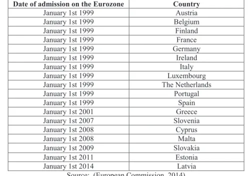
(21) CHAPTER 1- INTRODUCTION. 1.2 The Eurozone The European Union (EU) is a political and economic union of 28 countries (European Union, 2014a) with a single market through a standardized system of laws (European Union, 2014b) that apply in all member states. The EU has its genesis in the European Coal and Steel Community (ECSC) and the European Economic Community (EEC), created by the Inner Six countries in 1951 and 1958, respectively. The community and its evolutions have grown in size by the admission of new member states and in power by the addition of policy areas to its scope. The Treaty on European Union (1992), also known as Maastricht Treaty established the EU in 1993 and introduced European Citizenship. The most recent major amendment to the constitutional basis of the EU, the Treaty of Lisbon (2007), came into force in 2009. The Eurozone is an economic and monetary union that was established in 1999 and effectively materialized in 2002. Since December 2014, the Eurozone is composed of 18 member states that use the euro as their legal tender: Austria, Belgium, Cyprus, Estonia, Finland, France, Germany, Greece, Ireland, Italy, Latvia, Luxembourg, Malta, Netherlands, Portugal, Slovakia, Slovenia, and Spain. The Eurozone is the second largest economy in the world and, in an aggregated view, has a population of 330 million inhabitants. France, Germany, and Italy are the three most important economies accounting for the majority of the Union’s GDP. One of the main objectives encompassed in the management of this Economic and Monetary Union and the euro was the achievement of economic stability, because it encourages economic growth, which brings prosperity and employment. According to the established Economic and Monetary Union (EMU), EU member states coordinate their economic policies with the objective of maintaining economic stability. The European Central Bank (ECB) conducts the EU monetary policy with the aim of promoting low inflation in the Eurozone (European Commission, 2013a). Economic stability and low inflation create the environment prone to sustainable long-term growth, which benefits the Eurozone Member States.. 5.

(22) CHAPTER 1- INTRODUCTION. 1.3 Technology and innovation as drivers for economic growth The more developed countries compete, on an international level, between each other and also with less developed countries of low-wage economies that can produce products at a much lower cost and put them on the market. On the current market outline this can pose a competitive disadvantage for the former. Therefore international competition between economies, amongst many other aspects, has been fought between paradigms of advantage by innovation and technology and advantage by the form of low cost at the expense of low wages and other social indicators. In contrast, when the more developed countries were starting their early growth process, they were technologically much more advanced than the rest of the world. They could therefore maintain their advantage by designing and developing new technology at a rate defined by their own long-term economic growth requirements. In this context, a race for innovation advantage has emerged, where countries compete intensely on to achieve the highest levels of innovation-based economic growth (Wein et al., 2014). Many countries, to increase their competitiveness in this race, have implemented national innovation policies aimed at promoting the ability of companies and organizations in their economy to achieve increased innovation and productivity gains. Alternatively, other countries are trying to attain an advantage by engaging on innovation mercantilist practices that distort global trade by attempting to redirect the location of innovation activity to their territories at the cost of other countries (Ezell, 2011). East Asian and Northern European countries, along with the United States of America (US), are leading the world in this race for global innovation advantage. In a comparison of the US versus the EU, the US continues to outperform the EU in innovation capacity. This is illustrated in the EU's own Innovation Union Scoreboard released by the European Commission (EC) (2014), which concluded that the US innovation performance in 2014 is still superior to that of the EU countries. The focus on innovation by the EU was particularly noticeable with the definition and implementation of initiatives such as the Lisbon strategy (Lisbon European Council, 2000) and the new Europe 2020 Strategy (European Commission, 2010a). The Lisbon 6.

(23) CHAPTER 1- INTRODUCTION. strategy, also referred to as the Lisbon Agenda, is a strategic development plan of the EU approved by the European Council, which proposed the conversion of the economy of the EU into a more competitive and dynamic knowledge-based economy before 2010. This strategic objective should be able to promote lasting economic growth together with a quantitative and qualitative improvement in employment and greater social cohesion. The EU has made some progress towards the objective of investing 3 % of GDP in Research and Development (R&D). Nonetheless it contrasts with the remarkable growth of R&D intensity in the major Asian research-intensive countries. Despite this progress, most Member States remained far from the national 2010 targets they set for themselves as a result of the Lisbon Agenda in 2005 (Commission of the European Communities, 2005). From both theoretical and empirical perspectives, it is widely accepted that technology and technological advances are an essential component of innovation and economic growth. Currently there is a convergence of views between various authors with regard to the existence of a positive relationship between the level of technological development and economic growth of countries. Schumpeter (1943), with his classic 1943 book “Capitalism, Socialism and Democracy”, started a different take on economics and on the economy. For Schumpeter, technological change was fundamental for economic growth, and creative destruction was central in capitalism. In 1957, with the publication of the article "Technical Change and Aggregate Production Function" by Solow (1957), productivity growth of economies was mainly explained by the importance given to the introduction of technological innovations. In fact, innovation and knowledge began to be regarded as important sources of economic growth in countries, especially in developed countries, which have excelled in terms of growth in production, productivity, and international trade. Technology has been assumed as key for raising standards of living. And, in this matter, economic policies began to promote a process of development associated with technological capacitation and with innovation gains, as well as increased participation in international markets and, above all, the expansion and strengthening of the internal market. In reality the investment in R&D was considered strategic to ensure technological potential and as a result, innovation and economic growth. In addition to extending the possibility of achieving a higher technological level in companies and regions, which enables the introduction of new products or processes, it allows greater 7.

(24) CHAPTER 1- INTRODUCTION. growth and profitability. Nonetheless, the economic environment of the innovation process is fraught with uncertainties and risks and, in the course of investment decisionmaking in technology, economic operators take on even higher risks than the existing ones. It is commonly assumed that R&D activities generate knowledge which, if successful, can lead to the introduction of new technologies, processes or products with added value, and suitable for economic exploration. Countries, with their specificities, produce different outcomes from inputs related to innovation knowledge and technology and, as final output, economic growth increases the market value of goods and services produced, leading to the better economic performance of a country. Higher levels of standards of living, education, and health are usually associated with the better-performing countries. In the EU, the Lisbon Agenda (Commission of the European Communities, 2005) purposed a change of paradigm for the member states, focusing on the creation of knowledge as a catalyzer for economic growth. This initiative was planned under the assumption that the participating countries would dedicate capital to implement it. It wasn’t fully fulfilled at the end of the program, but public and private investment in R&D was growing up to the time of the economic crisis. Following the outbreak of the crisis, a majority of Member States maintained or increased their R&D investments, despite fiscal constraints, and overall R&D spending over GDP increased until 2010 (European Commission, 2013b). However, there were gaps between Member State performances. Furthermore, in Member States where the business sector was knowledge-intensive and internationally competitive, the government’s strategy to protect R&D spending helped maintain the level of private investment. However, this proved more challenging for countries suffering from sovereign debt crisis. In these countries liquidity constraints combined with an insufficiently innovation–friendly environment and a lower level of business demand for knowledge, prejudiced the effectiveness of the counter-cyclic measures to stimulate business investment (European Commission, 2013b). Nonetheless, the start of the recovery in 2010 was substantially stronger in countries which had previously invested the most in R&D and innovation, such as Germany, Finland and Sweden (European Commission, 2013b).. 8.