Numerical Simulations to Assess ART and MART Performance for Ionospheric Tomography of Chapman Profiles

Printed version ISSN 0001-3765 / Online version ISSN 1678-2690 http://dx.doi.org/OI: 10.1590/0001-3765201720170116

www.scielo.br/aabc | www.fb.com/aabcjournal

Numerical Simulations to Assess ART and MART Performance

for Ionospheric Tomography of Chapman Profiles

FABRICIO S. PROL1

, PAULO O. CAMARGO1

and MARCIO T.A.H. MUELLA2

1_{Universidade Estadual Paulista/UNESP, Departamento de Cartografia, Rua Roberto}

Simonsen, 305, 19060-900 Presidente Prudente, SP, Brazil

2

Universidade do Vale do Paraíba/UNIVAP, Laboratório de Física e Astronomia - IP&D,

Rua Shishima Hifumi, 2911, 12244-000 São José dos Campos, SP, Brazil

Manuscript received on February 15, 2017; accepted for publication on April 28, 2017

ABSTRACT

The incomplete geometrical coverage of the Global Navigation Satellite System (GNSS) makes the ionospheric tomographic system an ill-conditioned problem for ionospheric imaging. In order to detect the principal limitations of the ill-conditioned tomographic solutions, numerical simulations of the ionosphere are under constant investigation. In this paper, we show an investigation of the accuracy of

Algebraic Reconstruction Technique (ART) and Multiplicative ART (MART) for performing tomographic reconstruction of Chapman profiles using a simulated optimum scenario of GNSS signals tracked by

ground-based receivers. Chapman functions were used to represent the ionospheric morphology and a

set of analyses was conducted to assess ART and MART performance for estimating the Total Electron Content (TEC) and parameters that describes the Chapman function. The results showed that MART performed better in the reconstruction of the electron density peak and ART gave a better representation for

estimating TEC and the shape of the ionosphere. Since we used an optimum scenario of the GNSS signals,

the analyses indicate the intrinsic problems that may occur with ART and MART to recover valuable

information for many applications of Telecommunication, Spatial Geodesy and Space Weather.

Key words: Grid-based tomography, electron density, ionospheric profile, Chapman function, GNSS, TEC.

Correspondence to: Fabricio dos Santos Prol E-mail: fabricioprol@hotmail.com

INTRODUCTION

The Global Navigation Satellite System (GNSS) has emerged in recent decades as an effective technology for imaging the morphology and dynamics of the ionosphere. Important contributions of GNSS have been developed by many researches in order to provide valuable information of the

ionosphere in maps of Vertical Total Electron Content (VTEC) (Otsuka et al. 2002, Azpilicueta

et al. 2006, Hernández-Pajares et al. 2009, Durmaz

350-450 km above the Earth’s surface. Consequently,

the accuracy of the ionospheric delay to be used in GNSS positioning is compromised (Brunini et al. 2004) and GNSS data for applications that analyze the vertical morphology of the ionosphere

is restricted. However, due to the community’s

interest in recovering vertical information,

tomographic reconstruction techniques linked to

GNSS observations began to be used to reconstruct electronic density information.

The geometry of GNSS signals is not

completely sufficient to provide a unique and

independent solution to the ionosphere by using ionospheric tomographic algorithms (Bust and

Mitchell 2008). To overcome this geometric

deficiency, constraints or initial conditions of the ionosphere are imposed in the reconstruction method (Wen et al. 2012, Seemala et al. 2014,

Prol and Camargo 2016). However, the efficiency

of the ionospheric tomography is an issue that depends on the assumptions made in the tomographic reconstruction method. Simulated scenarios have been constructed to retrieve TEC observations with the main goal of assessing the efficiency of the tomographic algorithms using controlled assumptions so that the limitations of the ionospheric tomographic reconstruction methods can be outlined.

Austen et al. (1988) first performed ionospheric

tomographic reconstructions using simulated data, showing that the VTEC resulting from the

Algebraic Reconstruction Technique (ART) match the VTEC used as reference quite well. Another algebraic algorithm, the Multiplicative Algebraic Reconstruction Technique (MART), was first used by Raymund et al. (1990) for ionospheric imaging.

They used a simulated scenario to accurately

reconstruct the ionosphere using MART and showed

that the reconstruction was highly dependent on the initial guess of the ionosphere. Since then, many other simulations have been conducted to

analyze the efficiency of ionospheric tomographic

algorithms (Raymund et al. 1994, Howe et al. 1998, Mitchell and Spencer 2003, Thampi et al. 2004, Materassi and Mitchell 2005a, b, Wen et al.

2012, Chartier et al. 2014, Seemala et al. 2014) and

for making comparison between ART and MART

algorithms for ionospheric studies (Das and Shukla

2011). However, in these simulated studies, the analysis of the efficiency of the algorithms uses

climatological models to simulate the ionospheric morphology and/or depends on the real scenario of existing ground-based GNSS receivers used to retrieve the simulated observations of TEC. The climatological models compromise the number of distinct scenarios that can be simulated to represent the ionosphere in regional applications. Also, the GNSS geometry may not be enough for

high performance of ART and MART when using

real scenarios of ground-based GNSS receivers. Due to the lack of GNSS data for many networks, many voxels of the tomographic system are not illuminated and, then, it may not be possible to obtain a complete understanding of the intrinsic

problems of ART and MART for ionospheric

tomography.

Two aspects were considered in the analysis

of the ART and MART algorithms in this paper:

(1) a simulated optimum scenario of GNSS signals was used and; (2) a fully controlled simulation based on the Chapman function described distinct scenarios of the ionosphere. Since we used an optimum scenario for the GNSS signals geometry, the investigation highlights the intrinsic problems that may be expected from the solution obtained from ill-conditioned tomographic systems derived from ground-based GNSS receivers. We then have

a clear indication of the efficiency and limitations of ART and MART for the estimation of the Chapman profiles and certain parameters that describe the

Telecommunication, Spatial Geodesy and Space Weather, which make the analyses an important specification in the performance of ionospheric tomographic algorithms. Section 2 shows the

mathematical formulation of ART and MART.

Section 3 presents details of the methodology used to simulate the GNSS signals and the ionosphere. Section 4 presents the results of the numerical simulations and Section 5 shows the conclusions

about the use of the algebraic techniques.

ART AND MART FORMULATION

In Computerized Ionospheric Tomography (CIT), the principal parameter used to describe the ionosphere is the Total Electron Content (TEC), which for GNSS data is expressed as the integral

of the electron density (ne) along the path from the

GNSS satellite (s) to the receiving antenna (

r

a column whose cross-sectional area is equivalent

to 1 m². It can be written as (Seeber 2003):

s

e r

TEC

=

∫

n ds

(1)

and for using TEC in CIT, the ionosphere is broken down into a grid of cells (pixels or

voxels) and TEC is approximated to a finite sum.

Assuming the electron density (

n

j

and d_ij the path length of the GNSS signal i inside

the boundaries that intersect the cell

j

(1) can be formulated as (Prol and Camargo 2015):

1

J

i ej ij

j

TEC n d

=

=

∑

(2)

where j ranges from 1 to J (number of voxels

into the grid) and d_ij = 0 if the signal does not

intercept the corresponding cell. The distance d_ij

may be calculated from the projection of an IPP (Ionospheric Pierce Point) in each point where the signal transverses a grid cell. Therefore, algebraic

techniques are used to estimate n_e in each cell.

ART works by an iterative process. An initial

guess (K=0) for the electron density ( 0

e j

n ) is

obtained from initial conditions of the ionosphere, and the electron density for iteration K+1 is then calculated by the following expression (Austen et al. 1988, Pryse et al. 1998):

(

)

1 2 1 J _K i j ij e j K K

e j e j J ij

ij j

TEC d n

n n w d

d = + = − = +

∑

∑

(3)

where ne jK 1 +

is the electron density value

obtained from iteration K+1,

w

parameter and TECi is the TEC observation for

signal i usually derived from GNSS data. The

1

J K ij e j j

d n

=

∑ _{term is equivalent to a scan through each cell} from the ionospheric grid that calculates the TEC value of the correspondent initial condition of the ionosphere. The initial condition is usually obtained from empirical models of the ionosphere, such as

from the International Reference Ionosphere - IRI (Bilitza et al. 2011), to fill in each cell from the CIT

grid.

In ionospheric imaging, different versions

from ART are commonly applied, such as MART. While ART performs the iterations with a linear formulation, MART is an entropy-optimization

algorithm based on the following nonlinear iteration

(Raymund et al. 1990, Pryse et al. 1998):

/

1

1

ij max

w d d

K K i

e j e j J _K

ij e j j TEC n n d n + =     =  



∑

(4)

where d_max is the largest path length of the

respective signal. Even when

1 J

K

ij e j i

j

d n TEC =

>

∑ , MART

produces non-negative values so, at a first view, an advantage to using MART, instead of ART,

is the guarantee of non-negative values for the reconstructed image.

It is worth mentioning that the weighting parameter is usually determined by empirical experiments and used to control the convergence

2008). Pryse et al. (1998) adopted

w

=

0.2

three times for ART and six times for MART. In

the present work, the weighting parameter was adopted ten times smaller than used by Pryse et

al. (1998), i. e., w=0.02, but the iterative process 0.02

cycles through all ray paths one thousand times for

both ART and MART. This strategy was adopted

because a smoother solution is expected when reducing the weighting parameter and increasing the number of iterations (Wen et al. 2007). Also,

the iterations are performed with a fixed number of times for ART and MART in order to use the same configurations for the comparison between

the algorithms.

INVESTIGATIONAL METHOD

In the present study, we did not seek to analyze any seasonal behavior of the ionosphere, any particular

phenomena at a specific region and period or any

real scenario of a GNSS network. The intention

here is to analyze the differences and limitations of ART and MART for ionospheric imaging of Chapman profiles using a geometry that enables

high performance of the algorithms. We therefore created a simulated ionosphere using a Chapman function and a large number of signals with the same geometry as the ground-based GNSS receivers.

A two-dimensional (2D) ionospheric grid was structured with a pixel resolution of 1° in latitude by 20 km in altitude and the signals were constructed considering virtual GNSS receivers located at every 5° in geographic latitude and in the 50°W geographic longitude section. The GNSS signals were designed for an elevation angle that ranges from 15° to 85° with a 5° interval. The azimuths

were determined equals to 0° or 180°, making

it ideal for two-dimensional case simulations. Figure 1 illustrates the ionospheric grid, the virtual receivers and the coverage area of the signals designed for one receiver.

IRI was used to calculate parameters of a

Chapman function. The following formulation was

used (Rishbeth and Garriott 1969):

1 z e z

e m

n

=

n e

with:

(

)

s

h h z

H

−

= (6)

where the peak height h_m and the critical

electron density n_m were obtained from IRI2012

for each set of pixels that defines an ionospheric profile. In addition, we used a previous least square

adjustment procedure to estimate the scale factor

H_s using observations of electron density n_e.

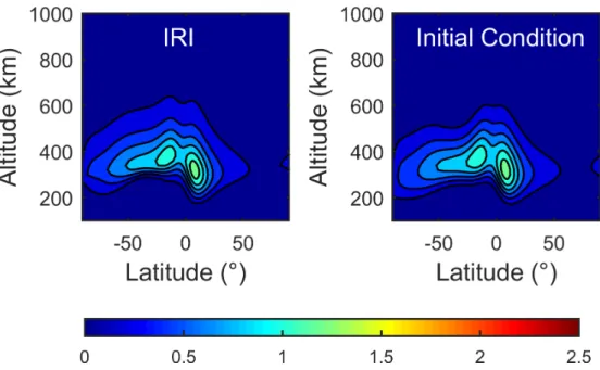
Figure 2 shows the input data from IRI (left

panel) for day 5, 2014, and the resulting image when performing the Chapman adjustment (right panel). This adjustment approach was performed using observations of electron density derived from

IRI and a function model based on equation (5). The

design matrix was built by calculating the partial derivative of the electron density in relation to the

scale height. The following equation was used:

1 _{z e}z z

e m

s s s

n z e

n e z

H H H

− −

− −  

∂ _{= −}

 

∂   (7)

where a distinct scale height was iteratively estimated for each set of pixels that describes an

ionospheric profile. As a result, electron density retrieved from IRI was not directly used to fill

in each pixel of the ionospheric grid. It was then possible to create a fully controlled ionosphere

with distinct values of the Chapman parameters h_m,

n_m and H_s to perform the simulations.

Figure 1 - Ionospheric grid with a spatial resolution of 1° x 20 km in latitude by altitude, virtual receivers located at every 5° (triangles) and the coverage area of the simulated GNSS signals for one receiver.

Figure 2 - Electron density obtained from IRI2012 in the left panel and Chapman adjustment to be used as initial condition for ART and MART in the right panel.

new images served as the expected ionosphere

to be reconstructed by ART and MART. It was

therefore possible to analyze the performance of

the algorithms performance using varied values of

the Chapman parameters and, consequently, create

distinct scenarios.

Visual and numerical analysis was carried out

for a total of four configurations, named Cases I, II,

III and IV. Cases I and II were developed to analyze

the performance of ART and MART for estimating

the critical electron density n_m, Case III analyzed

the peak height h_m and Case IV was carried out to

were made to assess the performance of ART and MART for visual interpretations of the ionospheric

profiles reconstructed in Cases I, II, III and IV. The numerical analysis was performed to analyze

quantitative differences between ART and MART

for calculating the parameters h_m, n_m and H_s and

also to calculate TEC for each input signal. As mentioned in the previous section, we used the

weighting parameter w equals 0.02 and performed

the reconstruction using 1000 iterations for all the

cases, which allowed us to analyze ART and MART using configurations that enables high performance

of the algorithms.

RESULTS OF THE SIMULATIONS

The next three sections present visual

comparisons between ART and MART for the

reconstruction of the electron density peak n_m, peak

height h_m and scale factor H_s. The following section

then shows the numerical results, presenting an

overview of ART and MART performance in

estimating h_m, n_m and H_s and also their accuracy in

retrieving TEC.

PEAK OF THE ELECTRON DENSITY

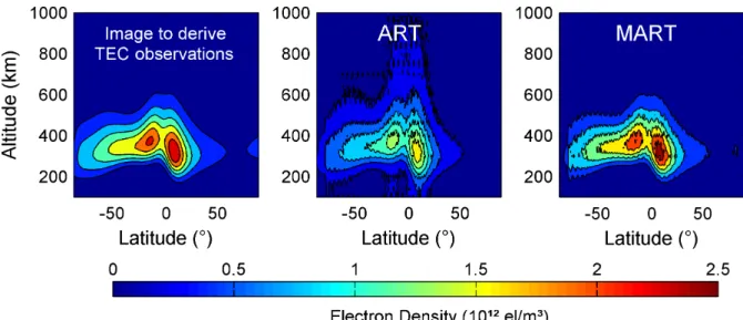
The first analysis (Case I) was constructed using

the initial condition shown in Figure 2 (right panel),

but the electron density peak n_m was doubled for

the image to retrieve TEC observations. Figure 3 shows the images used to retrieve TEC and also

the resulting reconstruction images from ART and MART algorithms. The limits of the color bar were set equal to the limits used in Figure 2, showing

a superior electron density in comparison to the

initial condition. We therefore applied the ART and MART algorithms to analyze its performance when

the initial condition underestimated of the intensity of the ionosphere.

From Figure 3, we can verify a superior visual

performance of MART in comparison with that obtained from ART. It can be seen that, when the

observed TEC is larger than the TEC from the

initial condition, ART overestimates the electron

density at high altitudes and underestimates it at

peak height. On the other hand, MART operates

with a reasonable performance, showing an electron density peak similar to the observed image.

When the observed value of TEC is lower than

the TEC of the initial condition, ART operates in an

opposite way to that observed in Case I. This can be seen in the results of Case II (smaller electron

density values), where Figure 4 shows that ART

underestimates the electron density in the upper altitudes and overestimates in the peak heights. This scenario was produced considering the electron

density peak n_m of each profile of the image to

retrieve TEC equal to half the image of the initial

condition. The initial condition of Case II therefore overestimated the intensity of the ionosphere.

In both analyses (Figures 3 and 4), MART reconstructed a more coherent image. However,

errors in the reconstruction occurred below -80° and above 80° in geographic latitude because the signals in this region were designed in only one direction, i. e., only signals with the azimuth of 180° were used below -80° and signals with an

azimuth equal to 0° above 80°. Thus, if only one

direction occurs with real geometry, the region must be analyzed with special care.

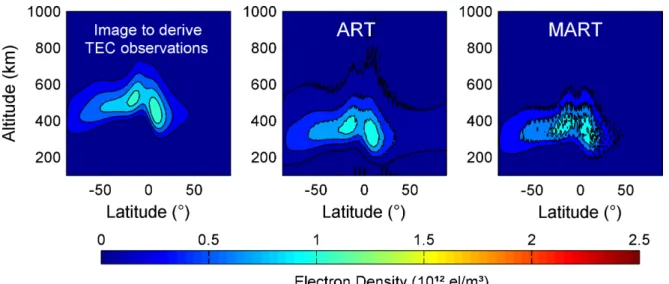
PEAK HEIGHT

Case III is shown in Figure 5, where the peak height of the image to retrieve TEC was set upwards in comparison with the initial condition. It can be noticed that the image to retrieve TEC observation has more concentration of electron density at high

altitudes. This was carried out by multiplying h_m by

a factor of 1.4 in each profile generating the image

for retrieving TEC observations. The 1.4 factor

was defined in order to make a significant elevation

Figure 4 - 2D algebraic technique performance in Case II (smaller electron density values). Figure 3 - 2D algebraic technique performance in Case I (larger electron density values).

peak height for the simulations, such as above 600 km. The maximum peak height obtained for the image to retrieve TEC was about 550 km. In this

way, we evaluated ART and MART for mapping

the vertical morphology of the ionosphere.

As can be seen, none of the algebraic

techniques detected the vertical variation, adding

to the limitation in estimating the peak height of

the ionosphere. A major difficulty in imaging the

uplifted ionosphere arises due to the absence of

signals in a horizontal direction and also because the vertical information does not make large changes in the tomographic system, making the observed TEC similar to the TEC from the initial condition.

Hence, the vertical information of tomographic

reconstruction is inherent to the initial condition used to represent the ionosphere.

Some improvement can be made by including

But special attention is given to ionospheric tomography using GNSS receivers located on the Earth’s surface, since it represents the largest number of TEC observations in tomographic reconstructions. It is relevant to say that the GNSS signals must fall within the grid for electron

density integration in TEC. However, for regional applications, many RO signals fall outside the grid, which reduces the number of RO signals that can

be used in tomographic applications.

SCALE HEIGHT

Case IV was carried out in order to check the

performance of ART and MART to represent the

shape of the ionosphere. The image to retrieve TEC observations for Case IV was obtained by doubling

the scale factor H_s used to build the image of the

initial condition of the ionosphere. ART and MART

were applied and Figure 6 presents the resulting images.

It can be seen that the shape variation in the image to retrieve TEC observations provided an increase of electron density in the peak height.

ART and MART were therefore more sensitive

in the regions of the electron density peak. It is

also worth mentioning that ART performed better

at representing the shape of the ionosphere, what

is as expected because MART was developed to

scrutinize the entropy of reconstructed images.

MART maximizes the intensity of electron density

in regions with high entropy and maximum entropy

occurs mainly at peak height. Consequently, the

electron density peak n_m was overestimated in Case

IV, mainly in the MART results.

NUMERICAL RESULTS

An overview of ART and MART performance in

estimating h_m, n_m and H_s is presented in Figure

7. The parameters h_m, n_m and H_s were calculated

at each latitude based on the ionospheric profiles

obtained from the image used for the initial

condition (green lines), the image to retrieve TEC

observations (black lines), the ART reconstructions (blue lines) and the MART reconstructions (red

lines). It is worth mentioning that TEC used as reference in the simulations were obtained with a large range of values, varying from 8 to 172 TEC

Units (TECU – 1016 _{el/m²) in Case I, 2 to 43 TECU}

in Case II, 4 to 80 TECU in Case III and 8 to 150 TECU in Case IV.

As can be seen in Figure 7 and similar to the

analysis made by Das and Shukla (2011), MART

performs better in estimating n_m. When using n_m

derived from the image to retrieve TEC observations as reference, we obtained the absolute mean of the

discrepancy of MART equal to 0.67 1011

el/m³ for

Case I and 0.28 1011 el/m³ for Case II. On the other

hand, the absolute mean of the discrepancy for ART

in Cases I and II was 4.6 1011 el/m³ and 2.4 1011 el/

m³, which leads us to the conclusion that MART performed about 87% better than ART at estimating

n_m. In Case III, both tomographic algorithms

presented a similar performance, showing an absolute mean discrepancy of 127 km and 130 km

for MART and ART, respectively. However, ART

presented a better performance in estimating the shape of the ionosphere in Case IV. The absolute

mean discrepancy for estimating H_s was equal to

85 km for MART and 55 km for ART, showing that ART performed about 53% better than MART.

As an indicator of the quality for estimating TEC using ART and MART, Table I shows the Root Mean Square Error (RMSE) and the absolute maximum discrepancy of TEC. The RMSE of the Reconstruction Techniques (RT) was obtained using the following equation:

(

)

1

RT obs RT

RMSE TEC TEC

N

= ∑ −

(8)

where the TEC reference was defined the

same as the TEC observations (TECobs) and N is the

Figure 6 - 2D algebraic technique performance in Case IV (shape variation). Figure 5 - 2D algebraic technique performance in Case III (height variation).

In general, both algorithms were capable of providing images that agree with the input observations within of a few TECU. The greatest discrepancies in the TEC reconstructions using both algorithms were obtained in Case III, which relates to the variations of the peak height, presenting a maximum discrepancy of 0.17 TECU and 0.39

TECU for ART and MART, respectively.

As can be seen in Table I, ART presented lower values in RMSE and in maximum differences. In

fact, based on the ART and MART formulations, a better performance is expected for ART in estimating the RMSE, such as discussed by Gordon et al. (1970) when applying the ART and MART

algorithms for reconstructing a varied number of

distinct objects. The expected ART solution is the one which minimizes the TEC differences between

the observed TEC and the TEC obtained through the iterations (

1

J K i ij e j

j

TEC d n

=

−∑ ), i.e., ART minimizes the

the other hand, MART is an entropy-optimization algorithm. The expected solution from MART is

the one with the maximum entropy, which occurs when the ratio between the observed TEC and the TEC obtained through the iterations (

1

/

J K i ij e j

j

TEC d n =

∑ ) is

close to 1. According to Raymund et al. (1990), by

maximizing the entropy, the reconstructed image is less likely to have erroneous artifacts introduced by

the reconstruction process. However, the entropy is not directly related to the RMSE. Therefore,

despite showing a better performance in visual

analysis for Cases I and II, MART showed a worse

performance on the TEC estimation.

It is possible to obtain a lower RMSE for MART reconstructions, but more iterations are

needed. Figure 8 shows a representative example

of the performance of ART and MART to estimate

TEC in terms of the iterations, where it is possible to notice that as the number of iterations increases,

the TEC RMSE of both algorithms decreases. Also, the ART reconstruction converged with less iterations than the MART reconstruction to obtain a minimum RMSE in the TEC estimation. Therefore,

for practical purposes, it is important to consider

that ART needs less iterations to obtain a minimum

error in TEC estimation when using the same weighting parameter.

CONCLUSIONS

ART and MART algorithms were analyzed for

the ionospheric tomographic reconstruction of

Chapman profiles using an optimum scenario of

GNSS signals tracked by ground-based receivers and a fully controlled ionospheric simulation.

Simulated results were produced to analyze specific

cases based on three parameters of the Chapman

function. MART presented a better performance in

the reconstruction of the electron density peak n_m

and ART gave a better representation for imaging

the shape of the ionosphere described by the scale

factor H_s. Both algebraic techniques reconstructed

the horizontal variations well. However, ART and MART presented limitations in representing the

vertical morphology of the ionosphere using GNSS geometry with receivers located at the Earth’s surface. In general, vertical information described

by the peak height h_m was highly dependent on

the initial condition of the ionosphere. But despite

significant errors on estimating h_m, both algorithms were capable of providing images that agreed well with the input TEC observations, providing a maximum error of 0.4 TECU.

Bearing in mind that we used an optimum scenario of GNSS signals and a fully controlled ionospheric simulation, the limitations pointed out in this paper may serve as an indicator of

the intrinsic errors of ART and MART for real

scenario of ground-based GNSS receivers. It is

reasonable to say that a relevant overview of ART and MART has been provided for future modeling

developments. In general, the analyses suggest

that the choice of using ART or MART depends on

the user application. If the user needs information

about peak electron density, MART performed better. However, MART presented a relatively worse performance than ART when estimating the shape of the ionosphere and ART reconstruction converged with less iterations than MART to

obtain a minimum error in the TEC estimation. Therefore, the simulated experiments suggest that

ART is a more useful algorithm for applications that requires solely TEC information. Also, in

TABLE I

RMSE and maximum discrepancy of TEC estimation by ART and MART. The units are in TECU.

Cases ART MART

RMSE Max RMSE Max

Case I 0.015 0.079 0.055 0.182 Case II 0.007 0.040 0.014 0.045 Case III 0.019 0.174 0.088 0.394 Case IV 0.010 0.056 0.072 0.329

ACKNOWLEDGMENTS

This work was jointly funded by Fundação de Amparo à Pesquisa do Estado de São

Paulo (FAPESP) under grant 2015/15027-7,

Coordenação de Aperfeiçoamento de Pessoal de

Nível Superior (CAPES) and Conselho Nacional de Desenvolvimento Científico e Tecnológico

(CNPq) under grant 2014/09240-7. The authors also acknowledge the use of the IRI model.

REFERENCES

AUSTEN JR, FRANKE SJ AND LIU CH. 1988. Ionospheric imaging using computerized tomography. Radio Sci 23(3):

299-307.

AZPILICUETA F, BRUNINI C AND RADICELLA SM.

2006. Global ionospheric maps from GPS observations

using modip latitude. Adv Space Res 38(11): 2324-2331. BILITZA D, MCKINNEL LA, REINISCH B AND

FULLER-ROWELL T. 2011. The international reference ionosphere today and in the future. J Geod 85(12): 909-920.

BRUNINI C, MEZA A, AZPILICUETA F, VAN ZELE MA, GENDE M AND DÍAZ A. 2004. A new ionosphere

monitoring technology based on GPS. Astrophys Space Sci 290(3): 415-429.

BUST GS AND MITCHELL CN. 2008. History, current state, and future directions of ionospheric imaging. Rev Geophys 46(1): RG1003.

CHARTIER AT ET AL. 2014. Ionospheric imaging in Africa. Radio Sci 49: 19-27.

DAS SK AND SHUKLA AK. 2011. Two-dimensional

ionospheric tomography over the low-latitude Indian

region: An intercomparison of ART and MART algorithms. Radio Sci 46(2): 1-13.

DURMAZ M AND KARSLIOĞLU MO. 2015. Regional

vertical total electron content (VTEC) modeling together with satellite and receiver differential code biases (DCBs) using semi-parametric multivariate adaptive regression

B-splines (SP-BMARS). J Geod 89(4): 347-360.

GORDON R, BENDER R AND HERMAN GT. 1970. Algebraic reconstruction techniques (ART) for

three-dimensional electron microscopy and X-ray photography.

J Theor Biol 29(3): 471IN1477-476IN2481.

HERNÁNDEZ-PAJARES M, JUAN JM, SANZ J, ORUS R, GARCIA-RIGO A, FELTENS J, KOMJATHY A, SCHAER SC AND KRANKOWSKI A. 2009. The IGS

VTEC maps: a reliable source of ionospheric information

since 1998. J Geod 83(3): 263-275. Figure 8 - The RMSE of TEC estimation by ART and MART

in each iteration of Case III (height variation), which is the

case with maximum RMSE.

Figure 7 - Performance of ART and MART for estimating nm, m

h _and

s

H in cases I, II, III, IV.

future works, RO data may be incorporated into the

tomographic reconstructions. A new analysis set

may be performed to verify the contribution of RO

HOWE BM, RUNCIMAN K AND SECAN JA. 1998.

Tomography of the ionosphere: Four-dimensional

simulations. Radio Sci 33(1): 109-128.

MATERASSI M AND MITCHELL CN. 2005a. A simulation

study into constructing of the sample space for ionospheric

imaging. J Atmos Sol-Terr Phys 67(12): 1085-1091. MATERASSI M AND MITCHELL CN. 2005b. Imaging of

the equatorial ionosphere. Ann Geophys 48: 477-482. MITCHELL CN AND SPENCER PS. 2003. A

three-dimensional time-dependent algorithm for ionospheric imaging using GPS. Ann Geophys 46(4): 687-696.

OTSUKA Y, OGAWA T, SAITO A, TSUGAWA T, FUKAO S AND MIYAZAKI S. 2002. A new technique for mapping

of total electron content using GPS network in japan. Earth, Planets Space 54(1): 63-70.

PRYSE SE, KERSLEY L, MITCHELL CN, SPENCER PSJ AND WILLIAMS MJ. 1998. A comparison of reconstruction techniques used in ionospheric tomography. Radio Sci 33(6): 1767-1779.

PROL FS AND CAMARGO PO. 2015. Review of tomographic

reconstruction methods of the ionosphere using GNSS.

Rev Bras Geof 33(3).

PROL FS AND CAMARGO PO. 2016. Ionospheric

tomography using GNSS: multiplicative algebraic

reconstruction technique applied to the area of Brazil. GPS

Solut 20(4): 807-814.

RAYMUND TD, AUSTEN JR, FRANKE SJ, LIU CH, KLOBUCHAR JA AND STALKER J. 1990. Application

of computerized tomography to the investigation of

ionospheric structures. Radio Sci 25: 771-789.

RAYMUND TD, FRANKE SJ AND YEH KC. 1994.

Ionospheric tomography: its limitations and reconstruction

methods. J Atmos Sol-Terr Phys 56(5): 637-655.

RISHBETH H AND GARRIOTT OK. 1969. Introduction to Ionospheric Physics. New York: Academic Press, 331 p. SEEBER G. 2003. Satellite Geodesy: foundations, methods

and applications. 2nd ed., Berlin, New York: Walter de

Gruyter, 589 p.

SEEMALA GK, YAMAMOTO M, SAITO A AND CHEN CH. 2014. Three‐dimensional GPS ionospheric tomography over Japan using constrained least squares. J Geophys Res

119(4): 3044-3052.

THAMPI SV, PANT TK, RAVINDRAN S, DEVASIA CV AND SRIDHARAN R. 2004. Simulation studies on the tomographic reconstruction of the equatorial and

low-latitude ionosphere in the context of the Indian tomography

experiment: CRABEX. Annales Geophysicae 22(10):

3445-3460.

WEN D, WANG Y AND NORMAN R. 2012. A new two-step

algorithm for ionospheric tomography solution. GPS Solut 16(1): 89-94.

WEN D, YUAN Y, OU J, HUO X AND ZHANG K. 2007.

Three-dimensional ionospheric tomography by an

improved algebraic reconstruction technique. GPS Solut