João Carlos Bernardo Oliveira Alves Santos
Licenciado em Ciências da Engenharia Eletrotécnica e de Computadores3-D Hybrid Localization with RSS/AoA in
Wireless Sensor Networks:
Centralized Approach
Dissertação para obtenção do Grau de Mestre em
Engenharia Eletrotécnica e de Computadores
Orientador: Marko Beko, Professor
Associado, Universidade Lusófona de Humanidades e Tecnologias
Co-orientador: Rui Dinis, Professor
Associado com Agregação, Faculdade de Ciências e Tecnologia
da Universidade Nova de Lisboa
3-D Hybrid Localization with RSS/AoA in Wireless Sensor Networks: Centralized Approach
Copyright © João Carlos Bernardo Oliveira Alves Santos, Faculty of Sciences and Technol-ogy, NOVA University of Lisbon.
"Mathematics, and perhaps mathematicians deal in the domain of the absolute and engineers live in the domain of the approximate. We are fundamentally interested in the practical. And so, frequently we make approximations, we cut corners, we omit terms and equations to get things that are simple
A c k n o w l e d g e m e n t s
In this section I would like to take the opportunity to express my gratitude towards ev-eryone who helped me through the process of developing and writing this dissertation.
First and foremost I would like to thank my adviser, Prof. Marko Beko, for his guid-ance, encouragement, and the enormous patience demonstrated over the last year.
I’m thankful toUniversidade Nova de Lisboa, Faculdade de Ciências e Tecnologiaand Departamento de Engenharia Electrotécnica e de Computadoresfor the opportunity and the conditions which allowed me to complete my education.
I would like to express my gratitude to Slavisa Tomic, a PhD student here at the uni-versity with many work done in this studied field, for his help in some crucial times.
To my dear colleagues and friends, specially, André Rosado, Diogo António, Tiago Dias and Francisco Cruz, thank you for always being there for me, through thick and thin. Without your friendship, support and motivation over the years, this journey would not have been the same.
And at last but not least, I would like to express my gratitude to my family, more specifically my mother and father, for all they have done that helped me become the man I am today. To my girlfriend Raquel, thank you for all the love and support, you have been the key person during this stage of my life.
A b s t r a c t
This dissertation addresses one of the most important issues present in Wireless Sensor Networks (WSNs), which is the sensor’s localization problem in non-cooperative and cooperative 3-D WSNs, for both cases of known and unknown source transmit powerPT.
The localization of sensor nodes in a network is essential data. There exists a large number of applications for WSNs and the fact that sensors are robust, low cost and do not require maintenance, makes these types of networks an optimal asset to study or manage harsh and remote environments. The main objective of these networks is to collect different types of data such as temperature, humidity, or any other data type,
depending on the intended application. The knowledge of the sensors’ locations is a key feature for many applications; knowing where the data originates from, allows to take particular type of actions that are suitable for each case.
To face this localization problem a hybrid system fusing distance and angle measure-ments is employed. The measuremeasure-ments are assumed to be collected through received signal strength indicator and from antennas, extracting the received signal strength (RSS) and angle of arrival (AoA) information. For non-cooperative WSN, it resorts to these mea-surements models and, following the least squares (LS) criteria, a non-convex estimator is developed. Next, it is shown that by following the square range (SR) approach, the estimator can be transformed into a general trust region subproblem (GTRS) framework. For cooperative WSN it resorts also to the measurement models mentioned above and it is shown that the estimator can be converted into a convex problem using semidefinite programming (SDP) relaxation techniques.
It is also shown that the proposed estimators have a straightforward generalization from the knownPT case to the unknownPT case. This generalization is done by making use of the maximum likelihood (ML) estimator to compute the value of thePT.
The results obtained from simulations demonstrate a good estimation accuracy, thus validating the exceptional performance of the considered approaches for this hybrid localization system.
Keywords: AoA, GTRS, RSS, SDP, wireless localization, WSN.
R e s u m o
Esta dissertação aborda uma das temáticas mais importantes de Redes de Sensores Sem Fios (RSSFs),que consiste na localização de sensores em RSSFs 3-D não cooperativas e cooperativas. Para ambos os casos de quando se conhece e de quando se desconhece a potência de transmissão dos sensoresPT.
A localização dos sensores numa rede é um dado essêncial. Existe um grande número de aplicações possíveis para RSSFs e o facto de os sensores serem robustos, terem baixo custo e não terem necessidade de manutenção faz com que este tipo de redes seja uma óptima solução para estudar e gerir ambientes adversos e de difícil acesso. O principal objectivo deste tipo de redes é o de recolher dados como temperatura, húmidade, ou qualquer outro tipo de dados, dependente do tipo de aplicação a que se destina a rede. O conhecimento da localização dos sensores é uma característica fundamental para diversas aplicações porque ao se saber a localização do sensor, sabe-se a localização dos dados re-colhidos e permite que determinadas acções possam ser tomadas com base na informação recolhida, variando de caso para caso.
Para fazer face a este problema de localização, implementou-se um sistema híbrido que combina medições de ângulos e distância. Assume-se que as medições são recolhidas através de um indicador de potência de sinal recebido e através de antenas, retirando a po-tência do sinal recebido e o ângulo de chegada do sinal. Para uma RSSF não-cooperativa, recorre-se a estes modelos de medições e seguindo o critério doleast squares(LS), é desen-volvido um estimador não convexo. De seguida, mostra-se que seguindo a aproximação dosquare range(SR), o estimador pode ser transformado numa estrutura do tipogeneral trust region subproblem(GTRS). Para uma RSSF cooperativa recorre-se aos mesmos mo-delos de medições, referidos em cima, e é mostrado que o estimador pode ser convertido num problema convexo recorrendo-se à técnica de relaxação semidefinite programming (SDP).
Também é demonstrado que os estimadores propostos têm uma generalização direta do caso em que se conhecePT para o caso em que não se conhece. Este generalização é feita recorrendo-se ao estimadormaximum likelihood(ML) que é usado para calcular o valor daPT.
Os resultados obtidos através das simulações realizadas demonstram a boa precisão na estimação da localização, validando o desempenho excecional das abordagens utilizadas
para um sistema de localização híbrido.
Palavras-chave: Ângulo de chegada do sinal, GTRS, localização sem fios, potência do sinal recebido, RSSF, SDP.
C o n t e n t s
List of Figures xv
List of Tables xvii
Listings xix
Acronyms xxi
1 Introduction 1
1.1 Background and Motivation . . . 1
1.2 Dissertation Objectives . . . 2
1.3 Dissertation Outline . . . 3
2 State of the Art 5 2.1 Introduction . . . 5
2.2 Issues in WSNs . . . 5
2.3 Localization Problem . . . 6
2.3.1 Stationary and mobility in sensor nodes . . . 6
2.3.2 Centralized and de-centralized networks . . . 6
2.3.3 Anchor-based and anchor-free algorithms . . . 6
2.3.4 Cooperative and non-cooperative networks . . . 7
2.3.5 Range-based and range-free localization . . . 7
2.4 Measurement Models . . . 11
2.4.1 RSS Model . . . 11
2.4.2 AoA Model . . . 13
2.4.3 ToA Model . . . 13
2.4.4 TDoA Model . . . 14
2.5 Hybrid Localization . . . 15
3 Hybrid Localization System Implementation 19 3.1 Introduction . . . 19
3.2 Problem Formulation . . . 19
3.3 Non-Cooperative Localization . . . 22
C O N T E N T S
3.3.2 Unknown source transmit power (PT) . . . 26
3.4 Cooperative Localization . . . 28
3.4.1 Known source transmit power (PT) . . . 29
3.4.2 Unknown source transmit power (PT) . . . 30
4 Performance Results 33 4.1 Introduction . . . 33
4.2 Complexity Analysis . . . 33
4.3 Simulations Results . . . 34
4.3.1 Non-Cooperative Localization Results . . . 35
4.3.2 Cooperative Localization Results . . . 39
5 Conclusions and Future Work 43
Bibliography 45
L i s t o f F i g u r e s
2.1 DV-Hop . . . 8
2.2 Centroid System . . . 8
2.3 APIT . . . 8
2.4 Triangulation . . . 9
2.5 Trilateration . . . 9
2.6 GPS-based localization principle . . . 10
2.7 3-D scenario illustration using AoA measurement . . . 13
2.8 One-way ToA . . . 14
2.9 Two-way ToA . . . 14
2.10 TDoA . . . 15
2.11 Range-based Localization . . . 16
2.12 Angle-based Localization . . . 16
2.13 Hybrid Localization in a 2-D scenario using RSS/AoA . . . 16
3.1 RSS measurements: short-range vs long-range . . . 24
3.2 AoA measurements: short-range vs long-range . . . 24
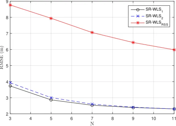
4.1 RMSE versus N comparison . . . 36
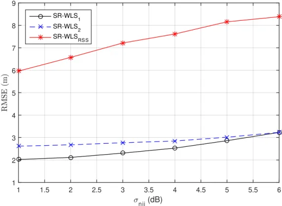
4.2 RMSE versusσnij comparison . . . 37
4.3 RMSE versusσmij comparison . . . 38
4.4 RMSE versusσvij comparison . . . 38
4.5 NRMSE versus N comparison . . . 40
4.6 NRMSE versus M comparison . . . 41
4.7 NRMSE versus R comparison . . . 42
L i s t o f Ta b l e s
2.1 Path Loss Exponents for Different Environments [19] . . . 11
4.1 Complexity Analysis Summary . . . 34
L i s t i n g s
A c r o n y m s
AoA Angle of Arrival.
APIT Approximate Point In Triangulation.
APS Ad-Hoc Positioning System.
BR-PLE Bias Reduction Pseudolinear Estimator.
GPS Global Positioning System.
GTRS Generalized Trust Region Subproblem.
LS Least squares.
ML Maximum Likelihood.
NLOS Non Line Of Sight.
NRMSE Normalised Root Mean Square Error.
PDF Probability Density Function.
PLE Path Loss Exponent.
PPS Precise Positioning Service.
RF Radio Frequency.
RMSE Root Mean Square Error.
RSS Received Signal Strength.
RTT Round-Trip Time.
SDP Semidefinite Programming.
SDR Semidefinite Relaxation.
SOCP Second Order Cone Programming.
AC R O N Y M S
SOCR Second Order Cone Relaxation.
SPS Standard Position Service.
SR Square range.
SR-WLS Squared range weighted least squares.
TDoA Time Difference of Arrival.
ToA Time of Arrival.
WLS weighted least squares.
WSN Wireless Sensor Network.
C
h
a
p
t
e
r
1
I n t r o d u c t i o n
1.1 Background and Motivation
Wireless Sensor Networks (WSNs) are a fairly explored theme, addressed and strongly consolidated in the literature that has been discussed over the past several years. The reason for that is related to the fact that there were huge advances in radio frequency and in electronics. Nowadays, the size of some components, constituting an integrated circuit (IC), are less than one millimetre making it possible to make smaller devices with the same, or even better, performance [1].
A WSN is built of sensor nodes, from a few to a large number of these small devices. The sensor nodes, generally spatially distributed trough a large area, are used to monitor different conditions such as temperature, sound, humidity or pressure, depending on
their applications. They can be used to just sense the data or also to actuate somehow. The development of WSNs was motivated by military applications such as battlefield surveillance. This motivation is correlated with the fact that, in general, this type of network does not need infrastructures as the common applications use a sink node that collects all the data sensed by the sensors and it is that node which computes and performs the needed actions. The set up time and the implementation cost are also big advantages of using these networks [2].
These networks are commonly used in intelligent buildings to, for example, reduce energy wastage by proper ventilation, air conditioning or the needed illumination of a given room. They can also be used for smoke or fire detection in buildings. Other well known applications are the detection of wildfires over large forests or the study and observation of biodiversity in wildlife. Nowadays, with the automation in the industry, the WSNs are also used to help processes. The sensors may be used to detect equipment failures, sense data and, depending on the equipment, activate some actuators. Lately,
C H A P T E R 1 . I N T R O D U C T I O N
the need of studying and monitoring oceans and rivers, led to new developments creating underwater and oceanographic WSNs in order to perform measurements far from the coastline, in the case of an oceanographic WSN, and to employ acoustic communications, pollution detection and to measure seismic activity in the case of underwater WSN [3].
As it has been seen, an infinity number of applications exists and the key feature for several of these applications consists in the location of the sensor which sensed some important data and consequently, an action is required. The main motivation for this dissertation is tied to the importance of knowing the sensors’ locations. The location knowledge of a sensed data allows an improvement of the overall operation of a network. For example, lets consider an automated irrigation system for agriculture. Irrigating just the dry areas increases the overall efficiency and reduces wasteful spendings.
The global positioning system (GPS) is the most accurate localization system used worldwide, but it is not very common to use it in every sensor node of a WSN. This is due to the fact that requires high precision, a complex process of timing and synchronization, and it cannot operate at indoor applications [1]. Instead of this system and in order to get low-cost solutions, it is common to implement systems using different types of
measurements, such as received signal strength (RSS), time of arrival (AoA), etc. The accuracy of these systems are much worse than a GPS-based localization system. Recently, instead of using just one type of the referred measurements, hybrid systems that fuse more than one type of these measurements were presented [4, 5, 6, 7]. These systems increase significantly the estimation accuracy while keeping the computational complexity low.
1.2 Dissertation Objectives
This dissertation addresses the sensors localization problem in a 3-D centralized WSN. The main goal is to analyse and evaluate a hybrid localization system performance using received signal strength (RSS) and angle of arrival (AoA) measurements. For that purpose, two schemes are considered: one non-cooperative and other cooperative localization. In each one, different estimators are developed with straightforward generalization from the
cases of known source transmit power (PT) to the cases of unknown source of transmit power (PT).
The estimators considered in this work are expected to have a good accuracy over a wide noise range. On that basis, several simulations were performed in order to evaluate these estimators. A comparison, between the considered hybrid system with a different
system using only one measurement type, is performed in every simulation in order to demonstrate the advantages of using this type of hybrid localization system instead of using other system with only one type of measurements.
1 . 3 . D I S S E R TAT I O N O U T L I N E
1.3 Dissertation Outline
The remainder of this thesis is organized as follows: Chapter 2 contains a literature re-view that covers fundamental concepts and the state of the art related to the different
concepts to be used throughout this dissertation. First, the main issues existing in WSNs are briefly described focusing on the sensors localization problem. The main concepts of classifications for localization schemes in WSNs are provided. Next, the GPS-based localization is introduced followed by the main alternatives consisting in major measure-ment models known and used in the literature. At the end of this chapter the concept of a hybrid localization scheme is given explaining the theoretical advantages of using it.
In Chapter 3 the localization problem that it is intended to be solved in this dis-sertation is formulated. The non-cooperative localization scheme, for both known and unknown source transmit powerPT, is presented and the steps needed to elaborate the developed estimators are explained. Next, the cooperative localization scheme, for both cases of known and unknown source transmitted powerPT, is addressed. It is shown how to transform the localization problem into a convex one and how this problem can be solved with convex optimization tools.
In Chapter 4, the computational complexity analysis of the considered algorithms in this dissertation is shown. Then, throughput evaluations were conducted through simu-lations of the proposed algorithms. A comparison between the estimators is performed and all the adopted considerations for the performed simulations are described.
Chapter 5 presents the final conclusions by highlighting the main contributions of this dissertation.
C
h
a
p
t
e
r
2
S t a t e o f t h e A rt
2.1 Introduction
The purpose of this chapter is to establish a theoretical framework of this dissertation. In Section 2.2 the known problems of WSNs are presented, giving more attention to the local-ization problem and different possible schemes are explained. Next, the most commonly
used measurement models that are employed to formulate the localization problem are shown in Section 2.4 giving more emphasis to the ones used in this dissertation in the following subsections.
At the end of this chapter, existing hybrid localization approaches, which use the measurements presented in 2.4, are presented.
2.2 Issues in WSNs
WSNs have several issues that affect their performance and design [8].TheHardware
de-sign must include a radio range as high as possible to ensure data connectivity; the Operating System should have inbuilt features to reduce the energy consumption; the MAC protocolsshould avoid collisions and other types of interferences thereby optimizing the energy consumption of sensors; theSynchronization protocolis needed to be robust to delays, in the communication process, and failures. When theDeploymentis random, as for example, the sensors are dropped by a plane in a harsh environment, despite of a short distance between two deployed sensors, they can be unable to communicate due to obstacles or interferences. To maximize the energy efficiency, theNetwork Layershould
provide a flexible platform to perform routing and data management. TheTransport Layer should have protocols that ensure the transmission order of fragmented segments.
These are some of the known problems that reside in WSNs. But one of the most
C H A P T E R 2 . S TAT E O F T H E A R T
important problems, not mentioned above, in these type of networks is the knowledge of theLocalizationof the sensors. This is the main topic of this dissertation and is described with more detail in the next section 2.3.
2.3 Localization Problem
The localization theme is a crucial issue in WSNs management and operation. The lo-calization procedure is defined as the task of determining the physical coordinates of a sensor node (or a group of sensor nodes) or the spatial relationship between nodes [1]. Without the knowledge of the sensors location, the sensed data can be meaningless in many applications. For example, in an irrigation system if it is not known which part of the ground needs to be watered, the whole crop can be spoiled. On the other hand, in a wildfire detection, if the sensor location, which detected the fire, is known, the responsible entities could act more quickly and efficiently.
There are several classifications for localization schemes. A network can be centralized or distributed, cooperative or non-cooperative, the sensor nodes can be mobile or station-ary, the localization algorithms may be anchor-based or anchor-free and range-based or range-free. These classifications are described with more detail below.
2.3.1 Stationary and mobility in sensor nodes
Most of the applications in WSNs uses static nodes, which means that, after their deploy-ment, they stay stationary. Mobile sensors require specific algorithms and due to there complexity, less designed mechanisms exist [9]. When compared static with mobile nodes, it is perceptible that for a static node, its location is computed only one time. However, for mobile nodes, due to their movement, the algorithms have to adapt and perform the location estimation at every moment, depending on the application.
2.3.2 Centralized and de-centralized networks
The localization schemes can be classified ascentralized, where information is passed to a central node, ordistributedwhere all sensors estimate their own positions. In a centralized scheme, computation is left for a central node, implying high energy efficient schemes. A
de-centralized or distributed scheme requires that each node processes its own data, thus increasing the energy consumption of the entire network [10].
2.3.3 Anchor-based and anchor-free algorithms
Other typical classification for localization schemes is if an algorithm is anchor-based or anchor-free. Ananchoris a sensor node who is aware of its location through manual configuration or using GPS. In an anchor-based algorithm anchors correspond to a small percentage of the nodes constituting a network and they are used to estimate the unknown
2 . 3 . L O CA L I Z AT I O N P R O B L E M
location of the other sensors (targets). In an anchor-free algorithm, instead of a global positioning of the nodes, one coordinate system must be established by a reference group of nodes [11].
For the sake of simplicity, in the remainder of the text, the sensors with known location will be calledanchorsand the sensors with unknown locationtargets.
2.3.4 Cooperative and non-cooperative networks
Considering a WSN constituted by anchors and targets, in a non-cooperative scenario each target only communicates with anchors, and each position is estimated at a time. On the other scenario, node cooperation allows direct communication between any two nodes which are within the communication range, and all targets are localized simultaneously [12].
For networks with few energy resources, where only some targets can communicate directly with anchor nodes, a node cooperation is necessary. This is also made to extend the sensors lifetime [13].
2.3.5 Range-based and range-free localization
The algorithms for nodes position estimation are divided in two major classes,range-free andrange-basedlocalization algorithms.
Arange-freelocalization uses the radio connectivity among nodes in order to infer their position instead of using distance or angle measurements as in range-based local-ization. The main techniques used for this type of localization are theAd-Hoc Positioning System (APS),Centroid System,GradientandApproximate Point in Triangulation (APIT), which are briefly presented in the following [1, 10, 14, 15].
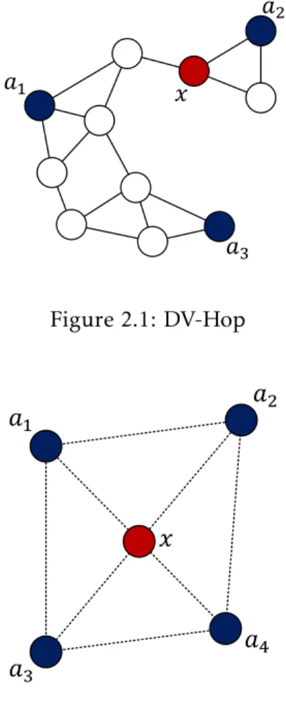
The APS can use theDV-hopmethod to estimate a target position [16]. This method (Fig. 2.1) is based on the distance vector protocol and the position estimation is done using hop count. To determine targets position, the anchors flood the network with their coordinates, generally obtained via GPS, and a hop count, which is incremented at each neighbour. Then, a correction factor is calculated in case an anchor obtains distances to another anchor. Having the anchors location and the correction factor, a target can perform its location estimation using trilateration, which will be discussed further.
The Centroid System (Fig. 2.2) presented in [17] uses multiple anchors to compute the target position. The anchors location are given to the target and its position is estimated as being the center of those multiple anchors.
In the Gradient algorithm presented in [18], anchors initiate a gradient that self-propagates and allow the target to estimate its distance from the anchor. Every target obtain informations of the shortest path from the anchors. The location of the target is computed through multilateration after estimating the distances from three different
anchors.
C H A P T E R 2 . S TAT E O F T H E A R T
𝑎1
𝑎3
𝑎2
𝑥
Figure 2.1: DV-Hop
𝑎
1𝑎
3𝑎
4𝑎
2𝑥
Figure 2.2: Centroid System
The APIT (Fig. 2.3), proposed in [14], requires a heterogeneous network where a small percentage of the devices are anchors equipped with high-power transmitters. The anchors form triangular regions between them and a target’s presence inside or outside these regions allow the target to refine down the area in which it can potentially remain.
𝑎1
𝑎3
𝑎4 𝑎2
𝑥
𝑎5
Figure 2.3: APIT
Arange-basedlocalization uses range measurements such asTime of Arrival (ToA),
2 . 3 . L O CA L I Z AT I O N P R O B L E M
Time Difference of Arrival (TDoA),Received Signal Strength (RSS)orAngle of Arrival (AoA), outlined in Section 2.4. Range-free localization techniques do not require additional hardware and are therefore a cost-effective alternative to these techniques. But the
trade-offbetween cost and accuracy is an important factor and the range-based techniques are
more appropriated to scenarios where the localization accuracy is a fundamental factor. The concepts commonly used to estimate sensors locations in this type of localization are based onTriangulation, Fig. 2.4, which measures the angles from more than one an-chor using AoA;Trilateration, Fig. 2.5, which measures the distance from three different
anchors using RSS, ToA or TDoA; and Multilateration, which is equal to the latter but where more than three anchors are used [1, 10]. In theory, the exact location is found
𝜙1 𝜙2
𝜙3
Figure 2.4: Triangulation
𝑑1
𝑑2
𝑑3
Figure 2.5: Trilateration
with one of those concepts, but in the real world, measurement errors occur due to the surrounding noise. This may lead to inaccurate localization and the need of an algorithm to solve this problem emerge.
GPS-based Localization
Global Positioning System (GPS)is the most well known localization technique used world-wide. Initially developed by United States Department of Defense (DoD) under the name NAVSTAR (Navigation Satellite Timing and Ranging) for military purposes, nowadays, the GPS has two levels of service [1].
1. Standard Position Service (SPS) which is a free positioning service available for civilian purposes. Tracking, surveillance and navigation, among many other ap-plications, using high quality GPS receivers based on SPS are capable of achieving precision of three meters.
C H A P T E R 2 . S TAT E O F T H E A R T
2. Precise Positioning Service (PPS) which is intended to serve the US and Allied mili-tary users with a more robust service that includes encryption and jam resistance. Instead of one signal, as SPS, the PPS uses two signals to reduce errors.
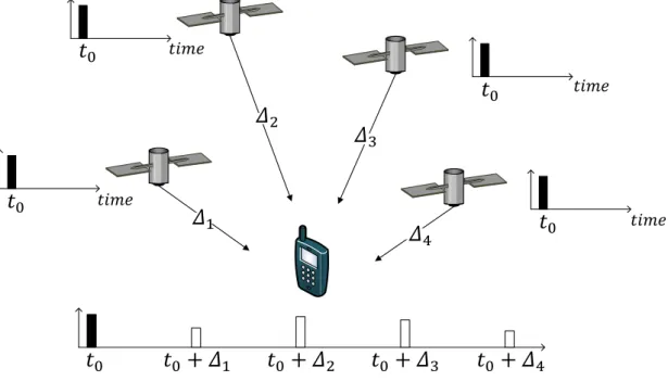
To obtain its location, a GPS receiver needs to have four satellites in line of sight. Each satellite broadcasts information with its own location, identity, status and the date and time of the signal sent under coded radio waves. The receiver and the satellites use very precise and synchronized clocks in order to generate at the same code exactly the same time. Comparing the generated code by the receiver with the one received by the satellite, the time of the travelled code is discovered and knowing that the radio waves travel at the speed of light, the distance between them can be determined based on ToA. The Fig. 2.6 represents this principle. After the receiver calculates its distance from each satellite, multilateration is used to obtain an accurate location.
𝛥
1𝛥
2𝛥
3𝛥
4𝑡
0𝑡
0𝑡
0𝑡
0𝑡
0𝑡𝑖𝑚𝑒
𝑡𝑖𝑚𝑒
𝑡𝑖𝑚𝑒
𝑡𝑖𝑚𝑒
𝑡
0+ 𝛥
1𝑡
0+ 𝛥
2𝑡
0+ 𝛥
3𝑡
0+ 𝛥
4Figure 2.6: GPS-based localization principle
The GPS receiver has several constraints for its use in every sensor of a WSN. The high power consumption is a major issue that affects the lifetime of each sensor; its cost could
make an entire network unaffordable and is limited to outdoor applications because of
its need for line of sight. In order to maintain low implementation costs, only a small fraction of sensors are equipped with GPS receivers (called anchors), while the remaining ones (called targets) determine their locations by using a kind of localization scheme that takes advantage of the known anchor locations.
2 . 4 . M E A S U R E M E N T M O D E L S
2.4 Measurement Models
This section summarizes the several types of measurement models used in range-based localization, giving more focus to the ones used in this dissertation. These models are required to formulate the localization problems and their usage depends on the available hardware.
2.4.1 RSS Model
It is known by [1, 19] that, a signal decays with the travelled distance following a power law of the separating length between sensors. The average received power Pij at i-th sensor with a distancedij from thej-th sensor, is approximated by
Pij=P0 dij d0
!−γ
, (2.1)
or
Pij(dB) =P0(dB)−10γlog10 dij
d0 !
, (2.2)
whereP0 is the received power at a short reference distanced0 andγ is the path loss exponent (PLE), typically ranged between 2 and 4 [20, 21]. In table 2.1 are shown the different values for PLE.
Table 2.1: Path Loss Exponents for Different Environments [19]
Environment Path Loss Exponent (PLE), γ
Free space 2
Urban area cellular radio 2.7 to 3.5 Shadowed urban cellular radio 3 to 5 In building line-of-sight 1.6 to 1.8 Obstructed in building 4 to 6 Obstructed in factories 2 to 3
The equation (2.2) can be rewritten as
Pij(dB) =P0(dB)−10γlog10 dij d0 !
+Xσ, (2.3)
for simulation purposes, whereXσ reflects the signal attenuation caused by fading, which is explained with more detail in the next sub-subsection 2.4.1.1.
Because of its low complexity and cost in software and hardware implementations, RSS is a popular method among the different types of measurements [22].
In [23] the authors proposed a weighted least squares (WLS) method when the source transmit power of a sensor and the PLE are unknown. In [24] to estimate the source transmit power along with the target’s location in a cooperative scenario, the authors resorted to a Semidefinite Programming (SDP) technique, which is a class of convex
C H A P T E R 2 . S TAT E O F T H E A R T
optimization. These are two examples of the research work in WSNs using the RSS model in the recent years.
Besides the type of ranging technique used to solve the localization problem it is necessary to appeal to mathematical models to compute the sensors location.
2.4.1.1 Log-Distance Path Loss Model
Path loss is a very important model in a wireless or radio communication system because it describes the signal attenuation between a transmit and receiver antenna (e.g. two sensorsiandj) due to multipath and shadowing caused by obstructions. Path loss model (in dB) is described as follows [19]
Lij(dB) = 10log10PT Pij
, (2.4)
whereLij is the path loss of the propagation channel between the sensorsi andj,PT is the transmission power andPij is the average received power between sensors. Replacing this equation in the RSS measurement model (2.2), theLog-distance Path Loss Model is obtained
Lij(dB) =L0(dB) + 10γlog10 dij d0 !
, (2.5)
whereL0represents the path loss at the short reference distance ofd0[19].
It has been showed in [25, 26] that the path loss at any distancedij in a same place is random and log-normally distributed about the mean distance-dependent value. So, in addition to this model, it is added aLog-normal Shadowingterm to consider the facts mentioned above, resulting in the equation
Lij(dB) =L0(dB) + 10γlog10 dij
d0 !
+Xσ, (2.6)
whereXσ is a zero-mean normal (Gaussian) distributed random variable with standard deviationσ and is denoted by
Xσ ∼N
0, σ2. (2.7)
As previously evidenced, the passage of the RSS model (2.3) to the log-distance path loss model (2.6) is straightforward, however, many authors use this latter model, as an alternative, to obtain their distance measurement through the RSS.
In [27], the authors investigated the noncooperative and cooperative schemes obtain-ing the location estimation of the targets through SDP estimators. For indoor localization, the authors in [28] used a WLS approach for cooperative and noncooperative schemes. However, to solve the localization problem, in the first scenario they relaxed that ap-proach as a mixed semidifinite and second-order cone programming (SD/SOCP) and in the second they solved the WLS approach through the bisection method. In [12], the authors also investigated the noncooperative and cooperative localization problems for known and unknown source transmitted power based on a SOCP approach.
2 . 4 . M E A S U R E M E N T M O D E L S
2.4.2 AoA Model
By definition, AoA is the angle measured between two sensors. To use this type of measurement it is necessary to equip the sensors with either a directional antenna or multiple antennas [29].
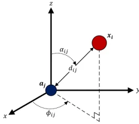
In a 3-D scenario, two types of angles are needed:azimuthandelevation(Fig. 2.7). A 2-D scenario only has two coordinates so, an elevation measure is not needed.
𝜙𝑖𝑗
𝑦 𝑧
𝒙𝒊
𝒂𝒋 𝛼𝑖𝑗
𝑑𝑖𝑗
𝑥
Figure 2.7: 3-D scenario illustration using AoA measurement
wherexi represents thei-th target node with unknown coordinates [xi1 xi2xi3],aj the j-th anchor node with known coordinates [aj1aj2aj3],φijis the azimuth angle,αijis the elevation angle anddij is the real distance between the nodes.
It can be readily shown, from Fig. 2.7, that the formulas for azimuth and elevation angles are, respectively
φij= arctan
xi2−aj2 xi1−aj1 !
+mij, (2.8)
and
αij= arccos
xi3−aj3 dij
!
+nij, (2.9)
wheremijandnijare introduced to represent possible measurement errors of both angles. In [30], the authors studied a 3-D scenario and proposed a method called bias re-duction pseudolinear estimator (BR-PLE) to estimate the sensor position. This approach jointly with [31, 32, 33, 34, 35], are some of the research work made with 3-D measure-ments of AoA. The 2-D scheme is very well substantiated in [36, 37, 38, 39, 40, 41].
2.4.3 ToA Model
The ToA is based on a simple law of physics stating that the distance between two sensors (e.g. an anchor and a target) can be obtained using the measured signal propagation time and its velocity [1, 42]. To do this, as was seen in GPS, both sensors need very accurate
C H A P T E R 2 . S TAT E O F T H E A R T
and synchronized clocks which increases the complexity and cost of the network. There are two different ranging schemes for this method.
𝑎
𝑡
𝑠𝑡
𝑎𝑥
Figure 2.8: One-way ToA
𝑎
𝑡
𝑠𝑡
𝑎𝑥
𝑡
𝑠2𝑡
𝑎2Figure 2.9: Two-way ToA
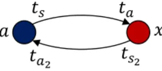
Theone-wayToA (Fig. 2.8) (used in GPS) measures the propagation time between the sensors computed as being the difference among the sending (ts) and arrival time (ta)
of the signal. The other possibility is to use thetwo-wayToA (Fig. 2.9) which measures the round-trip time (RTT) of the signal. The measured distances by these two methods, respectively, are computed as follows
dij = (ta−ts)×v, (2.10) and
dij=(ta2−ts)−(ts2−ta)
2 ×v, (2.11)
where dij is the distance between the i-th anchor and the j-th target, the variables t represent the times of sending and arrival signal andvis the velocity of the signal which is known, just depends on what type of signal is propagated (RF, acoustic or other).
Beyond these differences, with the one-way ToA, the target can compute its own
position because it estimates the distance between the target and the anchor (equation (2.10)). In the two-way ToA it is the anchor who estimates the distance among them (equation (2.11)) forcing a third message to be sent so that the target can compute its own location.
The approach of [43] considers non line of sight (NLOS) conditions and the authors proposed two relaxation methods based on semidefinite relaxation (SDR) and second order cone relaxation (SOCR) for two different cases where NLOS status is or is not
known.
2.4.4 TDoA Model
The TDoA representation (Fig. 2.10) uses two different types of signals, that travel with
different velocities [1, 44]. Both signals can be sent at a same time or after a fixed interval
(tw). The distance between the anchor and the target is determined by the latter (equation (2.12))
2 . 5 . H Y B R I D L O CA L I Z AT I O N
𝑎
𝑡
𝑠𝑡
𝑎𝑥
𝑡
𝑠2𝑡
𝑎2𝑣
1𝑣
2Figure 2.10: TDoA
where the variablesv represent the different velocities of the signals,ta andta2are the
times of arrival of the signals and tw is the time difference between the sent signals (tw=ts2−ts).
When compared to ToA, this method has the advantage of not needing clock synchro-nization between targets and anchors, but has the disadvantage that is required additional hardware depending of the different signal types used. Similarly to one-way ToA and
opposed to two-way ToA, in TDoA is the unknown target that estimate its own position.
2.5 Hybrid Localization
Due to measurement errors in each individual ranging technique, a hybrid localization scheme is thought to improve the localization performance by fusing more than one measurement type. A hybrid system has more available information, and by exploiting this information, a better accuracy in the localization procedure can be obtained. On the other hand, combining measurements implies an increased complexity of network devices increasing the network implementation costs [22, 42]. There are many possible schemes studied in the literature which are presented further in this section. Next, the hybrid localization scheme which uses RSS and AoA measurements is presented, since it is the main technique applied for this dissertation.
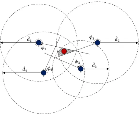
The range measurements can be obtained exclusively from RSS (Fig. 2.11) which has errors associated to the shadowing term. The angle measurements may be obtained through AoA (Fig. 2.12) which has associated errors given by antennas and digital com-passes due to its static accuracy. In the above mentioned figures, ˆdirepresents each range measurement, of an anchor, defining a circle as a possible location of the unknown target. Hence, a set of range measurements defines multiple circles and their intersected area contains a set of the target possible locations. Similarly, each angle measurement, φi, defines a line as the set of possible locations of the unknown target.
As it can be seen, both figures (Fig. 2.11 and Fig. 2.12) have a set of target possible locations, given by real conditions instead of an accurate and theoretical position esti-mation as shown in Fig. 2.4 and Fig. 2.5 where measurement errors are not considered. When used in conjunction, an improved performance is obtained as it can be seen from Fig. 2.13
In Fig. 2.13 one can see that when both measurements are integrated, the set of
C H A P T E R 2 . S TAT E O F T H E A R T
𝑑̂1 𝑑̂2
𝑑̂3
𝑑̂4
Figure 2.11: Range-based Localization
𝜙3
𝜙2
𝜙1
𝜙4
Figure 2.12: Angle-based Localization
𝑑̂1 𝑑̂2
𝑑̂3
𝑑̂4
𝜙3
𝜙2
𝜙1
𝜙4
Figure 2.13: Hybrid Localization in a 2-D scenario using RSS/AoA
2 . 5 . H Y B R I D L O CA L I Z AT I O N
possible solutions for the target’s location is reduced, proofing that hybrid systems are more likely to improve the estimation accuracy [45]. In this dissertation, the hybrid RSS/AoA system is employed but instead of 2-D, a 3-D scenario is used.
The authors in [6] proposed a selective weighted least squares (WLS) estimator for a RSS/AoA localization problem in a 2-D scenario for a non-cooperative network. By exploiting weighted ranges from the nearest anchors combined with the AoA measure-ments, they determined the unknown target location. In [46] the authors presented a WLS estimator for a 3-D non-cooperative localization problem using RSS difference fused
with AoA measurements. In [4, 5, 6] the authors only studied the hybrid RSS/AoA system for localization problem in a 2-D non-cooperative scenario only.
Other combinations of measures for hybrid localization systems are also studied in the literature. In [7, 47, 48] the authors made their approaches based on the combination between RSS and the two-way ToA measurements.
In [49], the authors introduced a new concept in hybrid localization. They combined a range-based with a range-free attribute, being the RSS and the DV-Hop the choices made to perform the unknown target localization in a 3-D scenario.
C
h
a
p
t
e
r
3
Hy b r i d L o c a l i z a t i o n S y s t e m I m p l e m e n t a t i o n
3.1 Introduction
In Section 3.2 the mathematical models to obtain the distance and angle measurements are presented for both cases of cooperative and non-cooperative scenarios and the target localization problem is formulated. Next, in section 3.3 the hybrid localization system implementation is addressed for the non-cooperative scenario for both cases of known and unknown source transmit powerPT. This chapter ends with the presentation of the proposed algorithm for the cooperative scenario.
3.2 Problem Formulation
A WSN withNanchors andMtargets is considered, where the anchors and the unknown targets locations are denoted, respectively, by
aj ∈R3, ∀j= 1,2, . . . , N , xi∈R3, ∀i= 1,2, . . . , M.
To determine the unknown targets location, a hybrid system fusing distance and angle measurements is employed in a 3-D scenario. Each sensor node has three coordinates (x, y and z) represented as
aj = [aj1aj2aj3], ∀j = 1,2, . . . , N , xi= [xi1xi2xi3], ∀i= 1,2, . . . , M.
The range measurements in this dissertation are assumed to be obtained exclusively through RSS information, more precisely, through the log-distance path loss model given in the previous chapter by equation (2.6). This assumption is made based on the fact that ranging based on RSS requires the lowest implementation costs. In this work, there are two different connections types, the target/anchor connection, which form a setA, and
C H A P T E R 3 . H Y B R I D L O CA L I Z AT I O N S YS T E M I M P L E M E N TAT I O N
the target/target connection, which form a setB. These sets are described as follows
A={(i, j) :kxi−ajk ≤R, ∀i= 1,2, . . . , M, j= 1,2, . . . , N}, and
B={(i, k) :kxi−xkk ≤R,∀i, k= 1,2, . . . , M, i,k},
whereRrepresents the communication range of any sensor of the network,xi andxk are the i-th andk-th unknown targets andaj is thej−thanchor. The normskxi−ajkand
kxi−xkkare the Euclidean norms and represent the distance between the two involved sensors.
Based on the sets mentioned above, the log-distance path loss model for each of set are modelled as:
LAij=L0+ 10γlog10 kxi−ajk d0
!
+nij, ∀(i, j)∈A, (3.1a)
and
LBik=L0+ 10γlog10 kxi−xkk d0
!
+nik, ∀(i, k)∈B, (3.1b) wherenij andnik are the log-normal shadowing terms modelled as zero-mean normal (Gaussian) distributed random variables with standard deviation (σijandσikrespectively). The distance between sensors must meet the constraint of being equal or greater than the short reference distance (d0) of a sensor.
In the rest of this work, without loss of generality, an assumption is made that the target/target path loss measurements, are symmetric, meaning thatLik=Lki ∀i,k.
After obtaining the RSS or the path loss measurements, is possible to estimate the distance between sensors. Knowing that the errors in equation (3.1a) and (3.1b) are represented by a random variable with zero-mean, the estimated distance for each set of sensors is given by
ˆ
dijA=d010 LAij−L0
10γ , ∀(i, j)∈A, (3.2a) and
ˆ
dikB =d010 LBik−L0
10γ , ∀(i, k)∈B. (3.2b)
The estimated distance in equation (3.2a) and (3.2b) can also be achieved through the maximum likelihood (ML) estimator [42].
The angle measurements needed for the 3-D scenario (azimuth and elevation) are obtained through AoA model which needs additional hardware as mentioned before. Applying the equation (2.8), for azimuth angle, to setsAandBresults in
φAij = arctan xi2−aj2 xi1−aj1 !
+mij, ∀(i, j)∈A, (3.3a)
3 . 2 . P R O B L E M F O R M U L AT I O N
and
φBik = arctan xi2−xk2 xi1−xk1 !
+mik, ∀(i, k)∈B, (3.3b)
wheremij andmik are noise terms. These terms, coming from two different sources, are the angle measurement errors and the orientation errors.
Similarly, when the equation (2.9) is applied for elevation angle, also to both sets, it results in
αAij = arccos xi3−aj3
kxi−ajk
!
+vij, ∀(i, j)∈A, (3.4a)
and
αikB = arccos xi3−xk3 kxi−xkk
!
+vik, ∀(i, k)∈B, (3.4b)
wherevijandvik are the same type of errors as the ones appearing in the equations (3.3a) and (3.3b) for the azimuth angle.
Although the errors stem from different sources, without loss of generality, they are
modelled as one random variable [29]. The errors of azimuth and elevation angle are modelled as follows
mij∼N0, σmij2, mik ∼N
0, σmik2 .
vij∼N0, σvij2, vik∼N
0, σvik2
.
These different measures, comprehending the estimated distances ( ˆdA
ij and ˆd B ik), the estimated azimuth angles (φAij andφBik) and the estimated elevation angles (αijAandαikB), are needed for all the investigated cases and only after their acquisition is possible to develop algorithms to estimate the unknown targets location. The combination of these measurements is the foundation of the hybrid system implementation.
Resorting to the equations presented in (3.1), (3.3) and (3.4), the observation vector is given as:
θ=hLT,θT,αTi ,θ∈R3(|A|+|B|),
whereL=hLAij, LBikiT,φ=hφAij, φikBiT,α=hαAij, αBikiT, and|A|and|B|denotes the number of elements in each set. Having the observation vector, the probability density function (PDF) is easily obtained as:
p(θ|x) =
3(|A|+|B|) Y
i=1
1
p
2πσi2 exp
(
−(θi−fi(x)) 2
2σi2 )
(3.5)
C H A P T E R 3 . H Y B R I D L O CA L I Z AT I O N S YS T E M I M P L E M E N TAT I O N
where
f(x) =
.. . L0+ 10γlog10
kxi−ajk
d0
.. .
L0+ 10γlog10kxi−xkk d0
.. . arctanxi2−xk2
xi1−xk1
.. . arctanxi2−xk2
xi1−xk1
.. . arccosxi3−aj3
kxi−ajk
.. . arccosxi3−xk3
kxi−xkk .. .
, σ=
.. . σnij .. . σnik .. . σmij .. . σmik .. . σvij .. . σvik .. . .
The ML estimator is the most popular approach since it has the property of being asymptotically efficient for enough data records allowing it to be implemented for
com-plicated estimation problems [50]. The conditional PDF, presented in (3.5) is maximized through the following ML estimator:
ˆ
x= arg min x
3(|A|+|B|) X
i=1 1
σi2[θi−fi(x)]
2, (3.6)
where ˆxis the resulting array from the ML estimation.
Although the ML estimator is approximately the minimum variance unbiased esti-mator [50], the LS problem presented in (3.6) is non-convex and has no closed-form solution. The main goal of this dissertation is to apply certain approximations so that it is possible to solve the localization problem presented in (3.6) in an efficient manner. For
non-cooperative WSN a non-convex estimator is proposed and for the case of cooperative WSN a convex one is proposed. These approaches, which are described with more detail in the following sections, not only efficiently solve the traditional RSS/AoA localization
problem, but they also can be used to solve the localization problem whenPT is unknown with a straightforward generalization.
3.3 Non-Cooperative Localization
In a non-cooperative localization scenario for WSN, comprising targets and anchors, the targets are only able to communicate with anchors, and one single target is located at a time. For this type of configuration, it is assumed that the targets are passive nodes,
3 . 3 . N O N - C O O P E R AT I V E L O CA L I Z AT I O N
which means that the sensors only report information, without processing it, through the emission of radio waves, and the anchors are the sensor nodes that collect all the radio measurements.
As the targets communicate exclusively with anchors, the setBis empty, so the equa-tions (3.1b), (3.2b), (3.3b) and (3.4b) to calculate, respectively, the path loss, the ap-proximated distance, the azimuth and the elevation angles for this set are not used in a non-cooperative localization scheme. For this type of scenario, it is assumed that the com-munication range (R) is high enough so that it is possible that the target can communicate with every anchor in the network.
To solve the localization problem presented in equation (3.6), a suboptimal estimator is developed, obtaining the exact solution through a bisection method. This estimator and the method are explained with more detail in the following subsections.
3.3.1 Known source transmit power (PT)
For the case when thePT is known, the first step is to assume that when the noise power is small enough, the following equations are obtained:
λAijkxi−ajk ≈d0, ∀(i, j)∈A, (3.7)
cijTxi−aj≈0, ∀(i, j)∈A, (3.8)
kijTxi−aj≈ kxi−ajkcosαijA, ∀(i, j)∈A, (3.9)
whereλAij = 10 L0−LAij
10γ ,c
ij = [−sin
φAij, cosφijA, 0]T andkij = [0, 0, 1]T ∀(i, j)∈A. The next step consists in squaring both sides of equation (3.7) resulting in
λAij2kxi−ajk2≈d02, ∀(i, j)∈A. (3.10) The weights,w=√wij, are introduced in order to give more importance to the nearest links. These weights are defined as:
wij= 1−
ˆ dijA P
(i,j)∈Adˆ A ij
, ∀(i, j)∈A, (3.11)
where ˆdijAis defined in equation (3.2a). The bigger importance given to the nearby links are due to the fact that both RSS and AoA short-range measurements are more reliable than the long-range measurements.
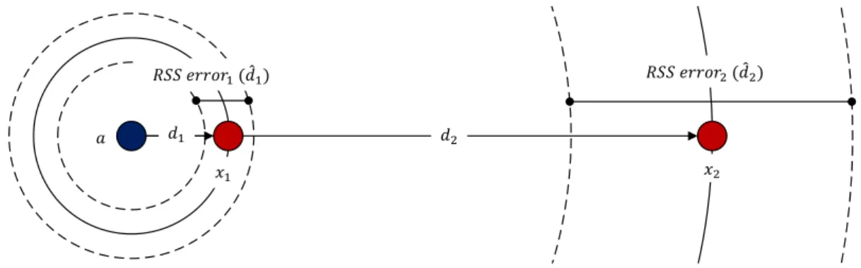
The RSS errors are considered to as multiplicative [42]. The standard deviation,σij, in dB, is constant throughout the distance but the multiplicative factor implies that, for example, when considering a multiplicative factor of 1.4, at a range of 10 meters, a measured range could be of 14 meters, meaning that the RSS error is of 4 meters. When
C H A P T E R 3 . H Y B R I D L O CA L I Z AT I O N S YS T E M I M P L E M E N TAT I O N
a longer range is considered, for example, 100 meters, the measured range could achieve the 140 meters, having an error of 40 meters, a factor 10 times greater that the previous example. This is the reason why RSS short-range measurements are more reliable. The Fig. 3.1 illustrates this idea.
The AoA errors, as opposed to RSS errors, are referred to as additive [42]. These are not the only source of errors in AoA measurements, multipath also impairs the location estimation. To illustrate this type of error and to give more emphasis to the importance of the closer links, the Fig. 3.2 shows an azimuth angle measurement made between an anchor and two targets located over the same line being one at a short-range and the other at a longer range. The real and the measured angles are denoted byφand ˆφrespectively. It is seen from Fig. 3.2 that the nearest target has better accuracy when the localization process is implemented when compared to the target farther away, despite the fact that the measured azimuth angle is the same.
𝑑1
𝑎
𝑥1 𝑥2
𝑅𝑆𝑆 𝑒𝑟𝑟𝑜𝑟1 (𝑑̂1)
𝑑2
𝑅𝑆𝑆 𝑒𝑟𝑟𝑜𝑟2 (𝑑̂2)
Figure 3.1: RSS measurements: short-range vs long-range
𝑎 𝑦
𝑥 𝑥1
𝑥2
𝐴𝑜𝐴 𝑒𝑟𝑟𝑜𝑟2
𝐴𝑜𝐴 𝑒𝑟𝑟𝑜𝑟1
𝜙 𝜙̂
Figure 3.2: AoA measurements: short-range vs long-range
The following step consists in the replacement ofkxi−ajkwith ˆdijAmodelled by (3.2a) and according to (3.8), (3.9), (3.10) and (3.11), the below squared range WLS problem is
3 . 3 . N O N - C O O P E R AT I V E L O CA L I Z AT I O N
formulated as:
ˆ
xi= arg min
xi
X
(i,j):(i,j)∈A wij
λAij2kxi−ajk2−d02
2
+ X
(i,j):(i,j)∈A wij
cTijxi−aj2
+ X
(i,j):(i,j)∈A wij
kTijxi−aj−dˆijAcosαAij2. (3.12)
The above SR-WLS estimator shares the same properties of the LS problem presented in (3.6) of being non-convex and of not having any closed-form solution. In spite of having these features, it is possible to express (3.12) as a quadratic programming problem resorting to the substitutionyi=hxiT, kxik2iT, thereby making it possible to efficiently
compute a global solution for this problem [51]. It is possible to rewrite the problem of (3.12) as:
minimize
yi kW
Ayi−bk2
subject to yiTDyi+ 2lTyi= 0,
(3.13)
where
W =I3⊗diag(w), D=
I3 03×1
01×3 0
, l=
03×1 −12
, A= .. . ... −2λAij2ajT λAij2
..
. ...
cijT 0 ..
. ...
kijT 0 .. . ...
, b=
.. . d02−λAij2kajk2
.. .
cijTaj
.. .
kijTaj+ ˆdijAcosαijA .. . ,
meaning thatA∈R3|A|×4,b∈R3|A|×1andW ∈R3|A|×3|A|∀(i, j)∈A. After having rewritten (3.12) as (3.13) it can be readily shown that not only the objective function but also the constraint in (3.13) have a quadratic form.
When both objective function and constraint are quadratic, the problem is known as a generalized trust region subproblem GTRS [51, 52, 53] and an exact solution can be obtained making use of a bisection procedure [51]. Although non-convex, the problems of this type have the necessaries and the sufficient optimum conditions from which efficient
solution methods may be achieved. For the bisection procedure, the optimal solution of (3.13) is given by
ˆ
y(λ) =(W A)T(W A) +λD−1
(W A)T(W b)−λl
, (3.14)
C H A P T E R 3 . H Y B R I D L O CA L I Z AT I O N S YS T E M I M P L E M E N TAT I O N
whereλis the only solution of
ϕ(λ) = 0, ∀λ∈I, (3.15) whereϕ(λ) and the intervalI are defined as follows:
ϕ(λ) = ˆy(λ)TDyˆ(λ) + 2lTyˆ(λ), (3.16) and
I=
− 1
λ1D,(W A)T(W A), ∞
, (3.17)
whereλ1is defined as being the highest eigenvalue ofD,(W A)T(W A).
The purpose is to use the bisection procedure to obtainλthat satisfies (3.16). After performing this procedure, the coordinates of the estimated target are obtained by re-placing the value ofλ, obtained by the bisection procedure, in equation (3.14), and the coordinate values are expressed by the first three elements of that equation.
Further considerations were taken into account for this bisection method such as limiting the maximum number of iterations to 30, in order to reduce the computational complexity of the algorithm. Such considerations are explained with more details in Chapter 4. In the remaining text, the algorithm presented in (3.13) will be denoted as "SR-WLS1".
3.3.2 Unknown source transmit power (PT)
Having an unknownPT is very common in WSNs, meaning that thePT is not calibrated. Generally this is done because calibration is not a priority and it is a way to maintain low implementation costs. The lack of knowledge of thePT corresponds to not knowingL0in (3.1a)[45, 54].
Similar to the previous case wherePT is known, the first step is to consider the noise power extremely low. Equations (3.8) stay equal but, due to the fact of not knowingL0, it is necessary to rewrite (3.7) as:
βijAkxi−ajk ≈ηd0, ∀(i, j)∈A, (3.18)
whereβijA= 10− LAij
10γ ∀(i, j)∈A, andη= 10− L0
10γ contains an unknown parameter (L
0) which, like the target position, also needs to be estimated. By squaring both sides of (3.18) it is obtained
βijA2kxi−ajk2≈η2d02, ∀(i, j)∈A. (3.19) The next step consists in the replacement ofkxi−ajkwith ˆdijA in (3.9) which corre-sponds to rewrite (3.9) as
βijAkijTxi−aj≈ηd0cos
αijA, ∀(i, j)∈A, (3.20)
![Table 2.1: Path Loss Exponents for Di ff erent Environments [19]](https://thumb-eu.123doks.com/thumbv2/123dok_br/16581469.738559/33.892.229.670.672.848/table-path-loss-exponents-for-di-erent-environments.webp)