Orientador: Professor Doutor João Mário Burguete Botelho Cardoso, Professor Auxiliar da Faculdade de Ciências e Tecnologia da Universidade Nova de Lisboa Co-orientador: Doutor Pedro Miguel de Almeida Talaia, Engenheiro de ID, CEiiA

Inês Maria Trindade Crespo

Licenciatura em Ciências da Engenharia Mecânica

Damage Propagation in Composite

Materials Meso-Mechanical Models

Dissertação para obtenção do Grau de Mestre em Engenharia Mecânica

Orientador: Professor Doutor João Mário Burguete

Botelho Cardoso, Professor Auxiliar da Faculdade de

Ciências e Tecnologia da Universidade Nova de Lisboa

Co-orientador: Doutor Pedro Miguel de Almeida Talaia,

Engenheiro de I&D, CEiiA

Júri:

Presidente: Prof. Doutor Pedro Samuel Gonçalves Coelho

Arguente: Prof. Doutora Marta Isabel Pimenta Verdete da Silva Carvalho Vogais: Prof. Doutor João Mário Burguete Botelho Cardoso

Doutor Bernardo Rodrigues de Sousa Ribeiro

i

Damage Propagation in Composite Materials

Meso-Mechanical Models

“Copyright” Inês Maria Trindade Crespo, FCT/UNL e UNL

v

Acknowledgment

To Dr. João Burguete Cardoso, the supervisor of this dissertation, for all the availability that he always had to receive me, for all he taught me, for his patient and for making available all resources needed for this dissertation. Even in the most difficult time he never stopped encouraging and helping me.

To all FCT-UNL Professors from the Mechanical and Industrial Engineering department, which contributed to the success of my academic career. They were the most important part of my graduation and I am very grateful to them.

To CEiiA and his collaborators, that received me and integrated me in their work ambient. They helped me whenever I needed, and advised me well.

To my Family, that always believe in my capacities. Especially my mother, who has always been by my side and always did her best to ever missed me anything.

vii

Abstract

Composite materials have a complex behavior, which is difficult to predict under different types of loads.

In the course of this dissertation a methodology was developed to predict failure and damage propagation of composite material specimens. This methodology uses finite element numerical models created with Ansys and Matlab softwares.

The methodology is able to perform an incremental-iterative analysis, which increases, gradually, the load applied to the specimen. Several structural failure phenomena are considered, such as fiber and/or matrix failure, delamination or shear plasticity. Failure criteria based on element stresses were implemented and a procedure to reduce the stiffness of the failed elements was prepared.

The material used in this dissertation consist of a spread tow carbon fabric with a 0°/90° arrangement and the main numerical model analyzed is a 26-plies specimen under compression loads. Numerical results were compared with the results of specimens tested experimentally, whose mechanical properties are unknown, knowing only the geometry of the specimen.

The material properties of the numerical model were adjusted in the course of this dissertation, in order to find the lowest difference between the numerical and experimental results with an error lower than 5% (it was performed the numerical model identification based on the experimental results).

Keywords:

ix

Resumo

Os materiais compósitos têm um comportamento bastante complexo, que é difícil de prever sob diferentes tipos de cargas.

No decorrer desta dissertação foi desenvolvida uma metodologia capaz de simular a ocorrência de falhas e a propagação de dano em provetes construídos com materiais compósitos. Esta metodologia utiliza modelos numéricos de elementos finitos, à escala meso-mecânica, criados através dos programas Ansys e Matlab.

A metodologia inclui a realização de uma análise incremental-iterativa, que aumenta, gradualmente, a carga aplicada no provete. Vários mecanismos de colapso foram incluidos, como a ocorrência de falha das fibras e/ou da matriz, delaminação ou plasticidade devida ao corte. Foram implementados critérios de falha baseados nas tensões dos elementos atraves de um procedimento para reduzir a rigidez dos elementos onde a falha ocorre.

O material usado neste trabalho consiste num tecido ultrafino de carbono com fibras orientadas a 0° e 90° e o modelo numérico analisado foi um provete de 26 camadas de tecido submetido à compressão. Os resultados numéricos foram comparados com os resultados

dos provetes ensaiados experimentalmente, cujas propriedades mecânicas são

desconhecidas, conhecendo-se apenas a geometria do provete.

As propriedades do material do modelo foram ajustadas no decorrer da dissertação, por forma a encontrar a menor diferença possível entre os resultados numéricos e experimentais com um erro inferior a 5% (foi realizada a identificação do modelo numérico face aos resultados experimentais).

Palavras-Chave: escala

xi

Table of Contents

Acknowledgment ... v

Abstract ... vii

Resumo ... ix

Table of Contents ... xi

List of Figures ... xiii

List of Tables ... xvii

List of Symbols ... xix

1. Introduction ... 1

1.1. Motivation ... 2

1.2. Objectives ... 2

2. Theoretical framework... 5

2.1. Composite Materials ... 5

2.1.1. Matrix ... 6

2.1.2. Fiber (reinforcement) ... 6

2.1.3. Textile composites ... 7

2.1.4. Spread Tow Carbon Fabric... 8

2.2. Damage in composite material ... 9

2.2.1. Fracture mechanism ... 10

2.2.2. Laminated damage mode ... 12

2.2.2.1. Longitudinal tensile fracture ... 14

2.2.2.2. Longitudinal Compressive fracture ... 14

2.2.2.3. Transverse fracture (with 𝛼 = 0) ... 16

2.2.2.4. Transverse fracture (with 𝛼 ≠ 0) ... 16

2.2.3. Failure criteria for plies ... 16

2.2.3.1. Maximum stress ... 16

2.2.3.2. Maximum strain ... 17

2.2.3.3. Tsai-Wu ... 17

xii

2.2.3.5. Hashin-Rotem ... 19

2.2.3.6. Puck ... 20

2.2.3.7. LaRC03/04 ... 21

2.3. Characterization of multi-scale models ... 27

2.3.1. Micro-scale models ... 29

2.3.1. Meso-scale models ... 29

2.3.1.1. Introduction to damage description in the meso-scale ... 30

2.3.2. Macro-scale models ... 32

3. Ply numerical model ... 33

3.1. Spread Tow Carbon fabric ply: initial model description ... 33

3.2. Mesh Convergence ... 34

3.3. Details of this first model ... 39

3.3.1. Shear and transverse compression plasticity ... 39

3.3.2. Delamination ... 41

3.4. Combined failure criterion ... 47

3.5. Incremental-iterative analysis... 48

3.6. Results ... 51

4. Numerical model of a specimen ... 57

4.1. Boundary conditions ... 58

4.2. Incremental iterative analysis ... 63

4.3. Results ... 67

4.3.1. Parameters adjustment ... 71

4.3.1.1. Results ... 72

4.4. Experimental results ... 76

4.4.1. Shear Plasticity ... 79

4.5. Comparison of Results ... 80

5. Conclusion ... 83

5.1. Complied objectives ... 85

5.2. Future Works ... 85

xiii

List of Figures

Figure 2.1 - Composite materials classification [5] ... 6

Figure 2.2 - Different reinforcement types [7] ... 7

Figure 2.3 - Different weave patterns of textile fabrics [9] ... 8

Figure 2.4 - An example of spread-tow carbon fabric [12] ... 8

Figure 2.5 - “Schematic of tow-spreading process with the help of air flow” [11]... 9

Figure 2.6 - Representative cross-section of: a) plain weave with spread tows; b) plane weave with regular tows ... 9

Figure 2.7 - Failure propagation modes[17] ... 11

Figure 2.8 - "Fracture surfaces and corresponding internal variables" [18] ... 12

Figure 2.9 - "Fracture surfaces and corresponding internal variables"[17] ... 13

Figure 2.10 - In-plane failure modes ... 14

Figure 2.11 - "(a) Fiber micro buckling between an elastic matrix in shear mode (up) and in tension mode (down); (b) kink band geometry; (c) real kink band" [18] ... 15

Figure 2.12 - Inter/fiber fracture modes [25] ... 20

Figure 2.13 - “Multi-scale damage and failure in fiber reinforced composites” [33] ... 28

Figure 2.14 - Different geometries for: (a) micro-scale, (b) meso-scale and (c) macro-scale [35] ... 29

Figure 2.15 - “Hypothesis of A) strain equivalence, B) stress equivalence and C) energy equivalence between the damage physical space and undamaged effective space”[18],[17] ... 31

Figure 3.1 - Simplified geometry of the - spread tow carbon fabric ply ... 33

Figure 3.2 - Representative elements (a) - Brick 8 nodes and (b) Brick 20 nodes [40] ... 35

Figure 3.3 - Simplified geometry for the mesh convergence ... 36

Figure 3.4 - Tension-number of elements for point A ... 37

Figure 3.5 - Tension-number of elements for point B ... 37

Figure 3.6 - Tension-number of elements for point C1 ... 38

Figure 3.7 - Tension-number of elements for point C2 ... 38

Figure 3.8 - Computational cost-number of elements ... 39

Figure 3.9 - Quasi-static and dynamic axial stress-strain responses from off-axis and transverse compression tests (for IM/8552 laminates) [21] ... 41

xiv

Figure 3.11 - “Normal contact stress and contact gap curve for bilinear cohesive zone material”

[45],[18] ... 43

Figure 3.12 - Boundary conditions used to test the cohesive elements implemented without contacts ... 44

Figure 3.13 - Final results of the delamination test (with cohesive elements without contacts) . 44 Figure 3.14 - Results of the delamination test with contact and cohesive elements for substep: (a) 6, (b) 22 and (c) 25... 46

Figure 3.15 - Comparison between Tsai-Wu a maximum stress failure criteria ... 48

Figure 3.16 - Incremental-iterative analysis for one ply under tensile loads (units of the initial parameters in m). ... 50

Figure 3.17 - Boundary conditions applied to the ply model ... 52

Figure 3.18 - Equivalent Von-Mises Stress Analysis at step 1 ... 52

Figure 3.19 - Equivalent Von-Mises Stress Analysis at step 2 ... 53

Figure 3.20 - Equivalent Von-Mises Stress Analysis at step 3 ... 53

Figure 3.21 - Equivalent Von-Mises Stress Analysis at step 14 ... 53

Figure 3.22 - Equivalent Von-Mises Stress Analysis at step 15 ... 54

Figure 3.23 - Stress-Strain results of the simulation of the ply model under tension loads ... 54

Figure 3.24 - Spread tow carbon fabric specimen after a tension test ... 55

Figure 4.1 - Geometry of the compressive specimen ... 58

Figure 4.2 - Results of the first compression test ... 59

Figure 4.3 - Results of the compression test with the cohesive properties changed and the boundary conditions (1) ... 60

Figure 4.4 - Results of the compression test with the cohesive properties changed and the boundary conditions (2) ... 61

Figure 4.5 - Results of the compression test with the cohesive properties changed and the boundary conditions (3) ... 62

Figure 4.6 - Numerical model and real specimen ... 63

Figure 4.7 - Incremental-iterative analysis for 26-plies compression specimen ... 64

Figure 4.8 - Equivalent Von-Mises Stress Analysis of a 26-plies compression specimen at step 4 ... 67

Figure 4.9 - Equivalent Von-Mises Stress Analysis of a 26-plies compression specimen at step 16 ... 68

Figure 4.10 - Equivalent Von-Mises Stress Analysis of a 26-plies compression specimen at step 17 ... 68

xvii

List of Tables

Table 3.1 - Spread tow carbon fabric ply dimensions ... 34

Table 3.2 - Elastic properties of IM7/8552 unidirectional laminates ... 34

Table 3.3 - Location of the evaluated points ... 36

Table 3.4 - Yield stresses of Hex-ply IM7/8552 unidirectional laminates ... 40

Table 3.5 - Cohesive material properties for IM7-8552 [38], [47] ... 43

Table 3.6 - Cohesive material properties, with critical energies density, for IM7-8552 [38], [48], [49]. ... 45

Table 3.7 - Unidirectional constants of the uniaxial tests used in the simulation of one ply under tension loads[17] ... 51

Table 4.1 - Dimensions of the compressive specimen ... 58

Table 4.2 - Elastic properties of IM7/8552 unidirectional laminates, for compression loads [38]. ... 59

Table 4.3 - Interlaminar cohesive properties changed ... 59

Table 4.4 - Boundary conditions (1) applied to the numerical model ... 60

Table 4.5 - Boundary conditions (2) applied to the numerical model ... 61

Table 4.6 - Boundary conditions 3) applied to the numerical model ... 62

Table 4.7 - Initial parameters of the 0º/90º spread tow carbon fabric compressive specimen .... 66

Table 4.8 - Unidirectional constants of the uniaxial tests used in the simulation of 26-plies specimen under compression loads. ... 66

Table 4.9 - Composite material mechanical properties used ... 67

Table 4.10 - Unidirectional constants of the uniaxial tests used in the simulation of 26-plies specimen under compression loads updated (𝑋𝐶 and 𝑌𝐶) ... 71

xix

List of Symbols

𝜎 Stress

𝜀 Strain

𝐸 Young modulus

𝑣𝑖𝑗 Poisson coefficient

𝐺𝑖𝑗 Shear modulus of elasticity for plane ij 𝐺𝐼 Energy release rate for mode I

𝐺𝐼𝐼 Energy release rate for mode II 𝐺𝐼𝐼𝐼 Energy release rate for mode III

𝛾 Classical surface energy

𝑈 Total potential

𝐴 Area

𝐾𝐼 Stress intensity factor 𝐺𝐼𝐶 Critical energy for mode I 𝐺𝐼𝐼𝐶 Critical energy for mode II 𝐺𝐼𝐼𝐼𝐶 Critical energy for mode III

𝑋𝑇 Failure stress under longitudinal tension 𝑋𝐶 Failure stress under longitudinal compression 𝑌𝑇 Failure stress under transversal tension 𝑌𝐶 Failure stress under transversal compression 𝑆𝐿 Failure stress under pure shear

𝛼 Angle of the fracture plane, fracture angle

xx

𝑓𝑖 Parameters used in Tsai-Wu failure criteria 𝐹𝑖𝑗 Parameters used in Tsai-Wu failure criteria

𝐹𝐼 Failure index

𝑆𝑇 Transverse shear strength

𝑆_𝐿𝑖𝑠 In-situ longitudinal shear strength 𝜏𝑒𝑓𝑓𝑇 Effective transverse shear

𝜏𝑒𝑓𝑓𝐿 Effective longitudinal shear

𝜂𝐿 _{Coefficients of influence in the longitudinal direction} 𝜂𝑇 _{Coefficients of influence in the transversal direction} 𝑌_𝑇𝑖𝑠 In-situ failure stress under transversal tension Λ_𝑗𝑗0 _{Parameters used in the LaRC03 failure criteria}

𝜑 Fiber misalignment angle

𝛾12𝑢 Engineering shear strain at failure

𝜓 Kink plane angle

𝐶𝑚𝑛𝑠𝑡0 Undamaged stiffness tensor

𝐼𝑖𝑗𝑘𝑙𝑚𝑛𝑠𝑡 Identity matrix

𝐷𝑖𝑗𝑘𝑙𝑚𝑛𝑠𝑡 Tensor formed by scalar damage variables

𝜎̃ Effective stress

𝜀̃ Effective strain

Ψ Free energy density

𝛿𝑛𝑐 Normal displacement jump at the completion of deboning; 𝛿𝑡𝑐 Tangential displacement jump at the completion of deboning;

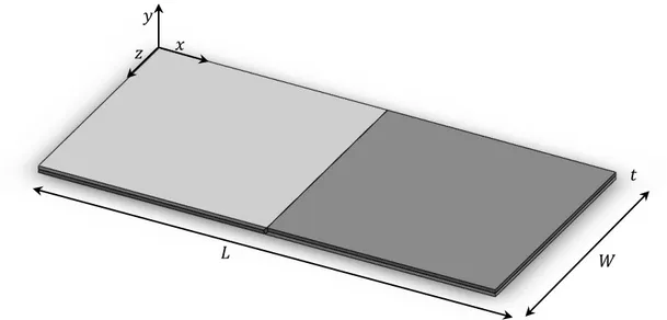
𝐿 Length

𝑊 Width

𝑡 Thickness

NFE Number of failed elements ∆_{𝑥𝑀𝑎𝑥} Maximum displacement applied

∆𝑥 Increment value

𝐷 Initial displacement in each iteration

𝑎𝑀𝑎𝑥 Maximum number of analysis

1

Introduction

Composite materials present great advantages over many metallic materials, causing them to be increasingly used in the aeronautical industry. The use of these materials has grown considerably in this industry, mostly, because of two important characteristics, which are low weight and high strength. However, to be able to take advantage of these characteristics it is necessary that the behavior of composite materials is well known so they can be used correctly.

The main goal of this dissertation is to study and predict the behavior of composite materials specimens (failure initiation and damage propagation) under certain loads, by developing an interface program methodology between MatLab and Ansys softwares (to perform the incremental-iterative analysis, which increase the applied loads on the numerical model at the same time as the stress results are evaluated). With this program, the numerical model of a ply model is first analyzed and subsequently, a 26-plies specimen under compression loads is studied.

The ply model is considered in Chapter 3 and its main purpose is to test de main features implemented in the program. In this chapter, a mesh convergence study is performed in order to evaluate the right element type and size to be used in subsequent numerical models. Also, cohesive and contact elements are implemented. Cohesive elements are used to simulate the delamination observed in the specimens tested experimentally and contacts are defined between different plies to avoid interpenetration (volume interference). Finally, it is proposed a combined failure criterion combining Maximum Stress and Tsai-Wu failure criteria and it is performed an incremental-iterative analysis of the ply, to find out the areas with higher stress concentrations.

2

numerical and experimental results. Finally, a comparison between numerical and experimental results is made.

The goal of this work consists in finding the material properties that provide similar results (with an error less than 5%) between experimental and numerical results, in order to validate the models presented here.

1.1.

Motivation

The subject of this dissertation arises after performing experimental tests in composite materials specimens subjected to tension and compression loads.

Before the experimental work, the behavior of the material was completely unknown and so there were no expectations regarding these results. After the experimental work, some doubts emerged concerning failure initiation and damage propagation. In order to study comprehensively the collapse behavior, it was proposed to implement a numerical model able to simulate these events that were observed in the specimens experimentally tested and obtain similar results.

This numerical models must be able to predict the failure initiation and the damage propagation, which are difficult to observe during the experimental tests, since everything happens fast.

Usually the knowledge of the composite materials behavior is acquired by the use of expensive and long-lasting experimental tests. The numerical simulation is capable to acquire the majority of this knowledge about the behavior of the composite material in a more economically way. Besides being less expensive than the experimental tests, virtual simulations have the ability to provide a better understanding of physical processes involved in the material behavior, since they provide much more information about the state of the system than the experimental test. Once the models are validated, the behavior of the material can be simulated, in the case of loads or boundary conditions change. Other advantages include the possibility to perform design optimization from the detailed knowledge of the material behavior.

Meso-scale models are so important, once they provide a set of effective material parameters needed in macro-scale models implementation.

1.2.

Objectives

The main objectives planned for this dissertation are presented bellow and each of them should be fulfilled in an objective and clearly way.

3  Implement cohesive and contact elements, in order to simulate delamination accurately;  Develop a methodology able to model the specimens tested and simulate the

experimental tests;

 Perform at least one analysis of a 26-plies compression specimen and provide the stress-strain curve results of this analysis;

5

Theoretical framework

2.1.

Composite Materials

According to Music and Witdroth [1], composite materials can be defined as a combination of, at least, two different materials with complementary properties. Each one of them has a function, one acts as a matrix, which maintains the material cohesive, while the second acts like a reinforcement, which provides resistance to the composite material.

Unlike some metal alloys, where different materials can be combined at the microscale and the components cannot be distinguished by the naked eye (it is an homogeneous material), the constituents of the composite materials remain separate and are easily distinguishable by the naked eye and this fact makes the composite materials heterogeneous materials [2].

The function of the matrix [3] is to hold the reinforcement in an orderly pattern and transfer the loads between the fibers that constitute the reinforcement, while the reinforcement gives the composite materials its desired properties

However, the global properties of these materials depends, not only, on the material properties of the components (matrix and reinforcement), but also, on the interface between them and the methods used in its production [1], [3]. It is expected that the composite material that results from a combination of two constituents has a balance of structural properties that is superior to either constituent material alone [4].

The main advantage of the composite materials is that, if well designed, they usually present the best qualities of their constituents and often some qualities that neither the constituents materials have [2]. Some of the properties that can be improved by producing a composite material are strength, stiffness, corrosion resistance, wear resistance, weight, fatigue life, temperature-dependent behavior, thermal insulation, thermal conductivity or acoustical isolation [2].

Figure 2.1 represents, schematically, the different types of composite materials that can be

6

Figure 2.1 - Composite materials classification [5]

2.1.1.

Matrix

The matrix of a composite material must ensure the connection of the reinforcements due to its cohesive and adhesive characteristics. When fibers are used as reinforcement, it protects them from the environment, from damage during manufacturing and operation and transfer the loads to and between the fibers [4].

Typically, the reinforcements are stronger and stiffer than the matrix. As a continuous phase, the matrix controls the transverse properties, interlaminar strength and elevated-temperature strength of the composite material. However it allows the strength of the fibers to be used in their full potential by providing effective load transfer from external loads to the fibers [4]. Additionally, the matrix provide an inelastic response in order to reduce de stress concentrations. So, the internal stresses are redistribute from the broken fibers [4].

The constituent material of the matrix, can be polymer, metal or ceramic, but the most widely used for aeronautical industry is polymer. Within the polymeric materials, the most common are epoxy resin and polyester. In this dissertation, the matrix that constitutes the composite material is an epoxy resin.

2.1.2.

Fiber (reinforcement)

The main function of a reinforcement is to provide superior levels of strength and stiffness to the composite materials [4].

Composites

Cement Reinforced Polimers

Reinforced with Particles

Particles

Reinforced by Dispersion

Reinforced with fibers

Continuous

Fibers Short Fibers

Aligned

7 Composite materials can contain the fibers in three different ways: particulate, continuous and discontinuous fibers, which are presented in the Figure 2.2. In the composite material with continuous fibers, the fibers provide all the strength and stiffness to the composite.

Music and Widroth [1] explain that, when using short fibers and particulates, the matrix must transfer the loads between the reinforcement more frequently, which results in a composite with low properties when compared to the composites with continuous fibers.

Graphite and carbon fibers are the most generally used advanced fibers, and graphite/epoxy or carbon/epoxy composite materials are now used commonly in aerospace structures [6]. It should be noted that the reinforcement of the composite material studied in this dissertation is composed by carbon fibers.

Figure 2.2 - Different reinforcement types [7]

2.1.3.

Textile composites

Textile composites are widely used in advanced structures in aeronautical, automotive and marine industries. It happens because they have good mechanical properties and attractive reinforcing materials with low fabrication cost and easy handling [8].

Since the material properties are anisotropic and inhomogeneous in nature, the parameters controlling the mechanical properties are numerous, such as fiber architecture, fiber properties or matrix properties [8].

Typically, textile composites are divided in three categories: woven fabrics, knitted fabrics and braided fabric [1]. However, the focus of interest in this dissertation will be the woven fabrics, once these are the most used textile composites in aeronautical industry [1], [8].

Within the textile composites, it can be found the in-plain weaves (2D), where each warp yarn passes alternately over and under each weft yarn, making the fabric produced symmetric [1].

The Figure 2.3 shows some examples of 2D woven patterns.

Some parameters, such as the weave architecture, yarn's dimension and spacing or yarn’s fiber volume fraction can affect the mechanical properties of the material.

8

Figure 2.3 - Different weave patterns of textile fabrics [9]

2.1.4.

Spread Tow Carbon Fabric

The material used in this dissertation is a spread tow carbon fabric, presented in the Figure 2.4.

This material presents many differences from the conventional carbon fabrics, with regular tows. To produce this material a conventional carbon fiber tow is thinned by increasing the width of the tow from 5 mm to approximately 25 mm, thus, reducing the weight per unit area by approximately 500% [10].

Figure 2.4 - An example of spread-tow carbon fabric [12]

The tow-spreading technology was developed by Industrial Technology Center in Fukui Prefecture. The operating mode of the tow-spreading technology consists of passing a tow though a spreading machine that is equipped with an air duct and a vacuum that sucks the air downward through the air duct, this process is shown diagrammatically in the Figure 2.5 [11]. By the use of this technology it can be produced unidirectional plies or woven fabric plies [10].

Plain

4 - Harness Satin 5 - Harness Satin

8 - Harness Satin Twill

9 Figure 2.5 - “Schematic of tow-spreading process with the help of air flow” [11]

The use of spread-tows results in a very thin plies with optimal in-plane and out-of-plane properties. As Hassan et. al. [10] referred, the ply thickness has a great importance in controlling composite material mechanical properties: “the thinner the ply the better the properties” [10].

Figure 2.6 - Representative cross-section of: a) plain weave with spread tows; b) plane weave with

regular tows

2.2.

Damage in composite material

Composites are complex engineered materials that often behave differently than common isotropic materials [12]. There are many types of damage in composite materials and the initial state of the materials is difficult, if not impossible, to characterize [2] Moreover, it is much more difficult to formulate a boundary-value problem to describe crack propagation in composite materials than in metals.

Polymer composites, which are generally used for manufacturing the aircraft components, due to their complex internal structure lead to different types of damage at many stages of their operational life. Defects that can emerge during the fabrication process of the composite materials are, for example, delamination, voids, particulates inclusion, resin-rich or resin starved, while during the aircraft operation damage are caused, mainly, by service loads and impacts.[13],[14].

a)

10

These damage can decrease the residual strength and durability of the structure leading to the failure (and then the fracture) of the material [13].

It should be noted the difference between damage and failure of the material. Both terms are ambiguous and it is important to understand the difference between them. As Oluwole. L said [15]: “damage leads to failure and failure leads to fracture”. When the material is damaged, due to problems during the fabrication process (voids, particles inclusion, resin rich, etc…) or impacts during its operation, it does not means that the material failed in service. Damage is a physical discontinuity in the material that can impair its normal functioning, which does not mean, necessarily, that the material is unusable. On the other hand, when the material fails, it cannot be used in service once it has lost its integrity. Finally when the fracture of the material happens, it means it was broken into two or more parts.

2.2.1.

Fracture mechanism

Fracture mechanism has evolved from the original work of Grifith [16]. Grifith recognized that defects (or damage) could lead to failure in materials, so he decided to propose and solve the idealized problem of a single crack in an infinite two-dimensional, isotropic, elastic medium under transverse load [16]. The solution obtained from the energy balance principle is given by:

𝜎 = √2𝐸𝛾_𝜋𝑎 (1)

where 𝜎, is the far-field stress that cause the crack to open and grow unstable under plane stress conditions, 𝑎 is the half crack length and 𝛾 represents the classical surface energy due to the breakage of bonds in the generation of new crack surface.

Later, Irwin (in 1950) generalized the form of equation (1) by introducing the macroscopic energy release rate, 𝐺, as an independent property [16]. Thus, for the same central crack problem:

𝜎 = √𝐸𝐺_𝜋𝑎 (2)

where,

11 being U, the total potential and A the crack area.

Further, Irwin greatly expanded the utility and applicability of the method by introducing the stress intensity factor, 𝐾_𝐼, with [16]

𝜎𝑖𝑗 = 𝐾𝐼

√2𝜋𝑟𝑓𝑖𝑗(𝜃)

(4)

This is the form of stress field near the linear elastic square root singularity and 𝐾_𝐼 (stress intensity factor) is given by

𝐾𝐼 = √𝜋𝑎𝜎 (5)

Then, in more general problems,

𝐾𝐼= 𝛼√𝜋𝑎𝜎 (6)

for mode I crack opening conditions. Similar forms follow for the mode II and mode III (the two shear modes) [16].

Fracture mechanics considers that a failure can grow in three different modes, mode I, mode II and mode III. The first mode is the opening mode, the second mode is the in-plane shear mode and the third is the out-of-plane shear mode [17], these three different modes are represented in the Figure 2.7.

Figure 2.7 - Failure propagation modes[17]

12

2.2.2.

Laminated damage mode

Consider composite material made of large unidirectional fibers (carbon or glass fiber, for example) embedded in polymer matrix (epoxy, for example). When a ply, without any notch, is tested, under various loading in the plane, the material fails in a manner and under certain tensions. The union of all the points, where the material suffers failure for the different stress states, generate a stress surface known as a failure criterion. In the interior of this surface are all the stress states that the material is capable to support without losing structural integrity. There are different failure modes in composite materials, which is a set of mechanisms of degradation that lead to the fracture of the material [17].

In Figure 2.8, where a unidirectional ply with the fiber oriented in the direction 1 is shown, is presented the different fracture surfaces under certain load states. The experimental observations lead to the conclusion that for an unidirectional ply under plane stress conditions there are, at least, four failure modes clearly identifiable. Figure 2.8 shows the fracture planes originated by each type of failure.

Figure 2.8 - "Fracture surfaces and corresponding internal variables" [18]

13 In Figure 2.9, it is represented the stress states that activated the respective failure modes, 𝐹_𝛼=0, 𝐹_𝛼≠0, 𝐹_𝐹𝑇 and 𝐹_𝐾𝐵 in the (𝜎₁₁− 𝜎₂₂), (𝜎₁₁− 𝜎₁₂) and (𝜎₂₂− 𝜎₁₂). 𝐹_𝛼=0 and 𝐹𝛼≠0 are the transverse failure modes or matrix failure while 𝐹𝐹𝑇 and 𝐹𝐾𝐵 are longitudinal failure modes or fiber failure.

However, due to the geometry of the material, there are 5 uniaxial tests (represented in the Figure 2.10) that are possible to perform in order to fully characterize the mechanical behavior of carbon fiber reinforced plastic: traction and compression in the direction of fibers (𝜎₁₁> 0 and 𝜎₁₁< 0, respectively), traction and compression in the transverse direction of fibers (𝜎₂₂> 0 and 𝜎₂₂< 0) and the pure shear test 𝜎₁₂ [17]. Each of these failure stresses is represented by 𝑋_𝑇, 𝑋_𝐶, 𝑌_𝑇, 𝑌_𝐶 and 𝑆_𝐿, respectively. These constants are used by the failure criteria, to define when the material fails under the action of external loads.

14

Figure 2.10 - In-plane failure modes

2.2.2.1.

Longitudinal tensile fracture

This is the simplest failure mode to identify, once that in the composite reinforced with fibers the loads are transferred by these ones and, when it fails, the loads have to be redistribute by the rest of the structure areas, which can lead to structural fracture [17], [18].

Composite materials with a high fiber fraction or in which matrix ultimate deformation is higher than in fibers leads to longitudinal fracture which begins in the fibers, in regions with defects. With the occurrence of the fracture of some fibers, the loads in the neighboring increase. These loads need to be transferred by shear, between the interface and the matrix, which cause matrix cracking and fiber pull-out. The higher the loads on the fibers, the greater will be the damage in the material, which lead to structural collapse [18]. So, it can be concluded that this type of failure occurs in both fiber and matrix.

2.2.2.2.

Longitudinal compressive fracture

When loads are applied in fiber direction, the laminate trend to fail by generation of kink band. This is the most common and most complex failure mode in this type of loading.

15 Some researches were conducted about the time independent compression failure and the first theoretical analyses made by Rosen [20] about microbuckling as a phenomenon of elastic instability. But, the results were above the critical stresses needed to occur microbuckling [20]. Consequently, some analysis were made with the aim of improve Rosen’s model. Argon (in 1972) and Bundiansky and Fleck (in 1993) included the yield effect in the matrix, fibers misalignment and fibers extensibility [20].

In the case of carbon fibers, several researchers observed the trend of the fibers to fail in shear mode instead of failing by bending from microbuckling. This produce a slant failure surface and consequently dislocation slip[18].

A kink band corresponds to the last state of damage under longitudinal compression. However there is a certain controversy about the generation of a kink band. The question is: It is a failure mechanism or it is the last stage of microbuckling? [17].

According to Sun and Tsai [19], it is assumed that in the kink band model, the compressive failure starts with the instability or excessive rotation of a misalignment fiber. This makes the fiber and matrix transfer high stresses, causing damage, separation of the components and matrix fracture [17].

Sun and Tsai [19], after comparing microbuckling and kink band models, concluded that in the microbuckling model it is assumed failure results from an instability located on fibers supported by elastic-plastic matrix. On the other hand, in kink band model failure is triggered by “yielding of plastic shear deformation of composites”.

Figure 2.11 - "(a) Fiber micro buckling between an elastic matrix in shear mode (up) and in tension

mode (down); (b) kink band geometry; (c) real kink band" [18]

16

2.2.2.3.

Transverse fracture (with

𝛼 = 0)

When the load is applied under transversal tension or in-plain shear, the failure progression occurs transversely to the laminate [17], [18].

These types of failures are developed essentially by transversal tension and in-plane shear. However, under high shear stress and with a moderate value of transversal compression, failures with the same orientation can be developed (with 𝛼 = 0) [17].

It should be noted that 𝛼 represent the fracture angle that is measured from normal to the top face and the fracture plane [21].

2.2.2.4.

Transverse fracture (with

𝛼 ≠ 0)

As Bessa referred [18], the behavior of the composite under transverse compression is very interesting, once there is a non-linearity in the stress-strain curve, which means that the composite materials plasticizes. Under transversal compression loads it is observed experimentally that the fracture angle varies with compression’s strength intensity and shear.

In fact, increasing the transversal compression loads, the fracture plain angle increases [17], [18]. Koerber [21] investigate the strain rate characterization of a unidirectional ply in transverse compression and in-plain shear using digital image correlation. Concluding that the behavior of a lamina subjected to shear loads is highly nonlinear.

2.2.3.

Failure criteria for plies

Failure criteria for plies determines, by the use of the failure stresses provided from the 5 uniaxial tests (𝑋_𝑇, 𝑋_𝐶, 𝑌_𝑇, 𝑌_𝐶 and 𝑆_𝐿), where lie the points that defines the failure of the ply through a set of functions. So, the failure criteria are used to predict the stress values for which the material fails under the action of external loads.

In this section some of the most used failure criteria in the prediction of composite materials failure will be presented, such as: maximum stress, maximum strain, Tsai-Wu, Tsai-Hill, Hashin-Rotem, puck or LaRC03/LaRC04.

2.2.3.1.

Maximum stress

17 𝑋𝐶 < 𝜎11< 𝑋𝑇

𝑌𝐶 < 𝜎22< 𝑌𝑇 𝑍𝐶 < 𝜎33< 𝑍𝑇

|𝜏23| < 𝑄 |𝜏13| < 𝑅 |𝜏12| < 𝑆

(7)

where 𝑋_𝑇, 𝑌_𝑇 and 𝑍_𝑇 are the tensile material normal strength in 𝑋, 𝑌 and 𝑍 directions, 𝑋_𝐶, 𝑌_𝐶 and 𝑍_𝐶 are the compressive material normal strength and 𝑄, 𝑅 and 𝑆 are the shear material strength. The failure appears when one or more equations in (7) are not satisfied.

2.2.3.2.

Maximum strain

Similar to the maximum stress failure criterion, the maximum strain can be expressed as [22]:

𝜀1𝐶< 𝜀11< 𝜀1𝑇 𝜀2𝐶 < 𝜀22 < 𝜀2𝑇 𝜀3𝐶 < 𝜀33 < 𝜀3𝑇

|𝛾23| < 𝑄𝜀 |𝛾13| < 𝑅𝜀 |𝛾12| < 𝑆𝜀

(8)

where 𝜀_1𝑇, 𝜀_2𝑇and 𝜀_3𝑇 are the tensile material normal failure strains, 𝜀_1𝐶, 𝜀_2𝐶 and 𝜀_3𝐶 are the compressive material normal failure strains and 𝑄_𝜀, 𝑅_𝜀 and 𝑆_𝜀 are the material shear failure. Violation of any of equations (8) indicates the material failure.

2.2.3.3.

Tsai-Wu

Tsai-Wu failure criterion is a quadratic and interactive stress-based criterion that identifies failure. This criterion is defined based on the tensile failure that occurs due to the five possible uniaxial testes, which are longitudinal tension and compression, transversal tension and compression and shear.[18], [17], [22], [23].

18

However, Tsai-Wu criterion does not distinguish between distinct modes of failure that are present in composite material [24].

This criterion can be expressed by a symmetric second order tensor:

𝑓(𝑥) = [ 𝑓1 𝑓2 𝑓3 0 0 0 ] 𝑇 [ 𝜎11 𝜎22 𝜎33 𝜎23 𝜎13 𝜎12]

+ [ 𝜎11 𝜎22 𝜎33 𝜎23 𝜎13 𝜎12]

𝑇 [ 𝐹11 𝐹12 𝐹13 0 0 0 𝐹12 𝐹22 𝐹23 0 0 0 𝐹13 𝐹23 𝐹33 0 0 0 0 0 0 𝐹44 0 0 0 0 0 0 𝐹55 0 0 0 0 0 0 𝐹66] [

𝜎11 𝜎22 𝜎33 𝜎23 𝜎13 𝜎12]

< 1 (9)

It is assumed that the material is transversally isotopic, which means that 𝑓₂= 𝑓₃, 𝐹₁₂= 𝐹₁₃, 𝐹22= 𝐹33, 𝐹55= 𝐹66 and 𝐹44=𝐹22−𝐹₂ 23 [17].

The parameters 𝑓 and 𝐹 in (9) are obtained from the failure stresses by the following expressions:

𝑓1=_𝑋1

𝑇−

1

𝑋𝐶 (10)

𝑓2=_𝑌1

𝑇−

1

𝑌𝐶 (11)

𝐹11=_𝑋1

𝑇𝑋𝑐 (12)

𝐹22=_𝑌1

𝑇𝑌𝐶 (13)

𝐹66=_𝑆1

𝐿2 (14)

𝐹12= −0.5_𝑋

𝑇2 𝑜𝑟 𝐹12= −

0.5

√𝑋𝑇𝑋𝐶𝑌𝑇𝑌𝐶 (15)

19

2.2.3.4.

Tsai-Hill

Tsai-Hill failure criterion is an adaptation of the Von-Mises criterion [25], [26]. As Tsai-Wu failure criterion, Tsai-Hill failure criterion is not associated with failure modes and it also considers that the 1, 2, 3 directions are not aligned with the principal directions.

Since the composites are transversally isotropic, this criterion reduces to:

(𝜎_𝑋11₂)2+ (𝜎_{𝑌 )}22 2−𝜎_𝑋1𝜎₂2+ (𝜎_𝑆12

𝐿)

2

< 1 (16)

here, 𝑋 = 𝑋_𝑇 when 𝜎₁₁ is positive and when it is negative, 𝑋 = 𝑋_𝐶. The same happens in the second direction, if 𝜎₂₂> 0 then 𝑌 = 𝑌_𝑇, but if 𝜎₂₂ < 0 then 𝑌 = 𝑌_𝐶.

2.2.3.5.

Hashin-Rotem

Hashin created the need for failure criterion that are based on failure mechanism [27]. He developed two different failure criterion, one of them was related to fiber failure and the other one was related to matrix failure [27].

In 1978 [28], [17], [29], [25], Hashin and Rotem developed a failure criterion for unidirectional laminates submitted to cyclic loads, distinguishing tensile loads from compressive loads. This criterion regards that failure of the material happens when the following equations are not satisfied:

𝜎11< 𝑋𝑇 if 𝜎11> 0

−𝜎11< 𝑋𝐶 if 𝜎11< 0

(𝜎_𝑌22

𝑇)

2 + (𝜎_𝑆12

𝐿) 2

< 1 if 𝜎22> 0

(𝜎_𝑌22

𝐶 )

2 + (𝜎_𝑆12

𝐿) 2

< 1 if 𝜎22< 0

(17)

Later, Hashin introduced the failure criterion for fibrous composites under a three dimensional stress state.[25], [29]

20 (𝜎11

𝑋𝑇) 2

+𝜎122 + 𝜎132

𝑆_𝐿 2 < 1, 𝑖𝑓 𝜎11> 0

−𝜎11< 𝑋𝐶, 𝑖𝑓 𝜎11< 0

(𝜎2_𝑌+ 𝜎3

𝑇 )

2

+𝜎232 − 𝜎2𝜎3 𝑆𝑇2 +

𝜎122 + 𝜎132

𝑆𝐿2 < 1, 𝑖𝑓 (𝜎2+ 𝜎3) > 0

[(_2𝑆𝑌𝐶 𝑇)

2

− 1]𝜎2_𝑌+ 𝜎3

𝐶 + (

𝜎2+ 𝜎3 2𝑆𝑇 )

2

+𝜎232 − 𝜎_𝑆 2𝜎3

𝑇2 +

𝜎122 + 𝜎132

𝑆_𝐿2 < 1, 𝑖𝑓 (𝜎2+ 𝜎3) < 0

(18)

where 𝑆_𝑇, represents the shear in 23 plain. The approximation describes the basic failure mechanisms but it is not capable to describe the kink band formulation [17], [24]

2.2.3.6.

Puck

The principal difference between puck criterion and Hashin [17], [25], criterion is that, in this one, three modes matrix cracking are considered, differing in the angle between the fracture plane on the lamina and the type of load which causes the fracture, as seen in Figure 2.12.

Puck’s criterion [30], identifies the fiber failure and inter fiber failure in a unidirectional composite. He separates, not only the inter fiber failure in three physical modes, but also the fiber failure in two different modes (tensile fiber failure and compressive fiber failure).

21

2.2.3.7.

LaRC03/04

Similarly to what happens in Puck’s criterion, LaRC03 and LaRC04 [17] criteria consider the different processes in each failure mechanism.

In these criteria it is taking into account that the transverse strength varies in function of the elastic characteristics of the laminate [17].

The principal difference between LaRC03 [27] and LaRC04 failure criterion [31] is that LaRC03 failure criterion just takes into account the in-plane tensions, while LaRC04 allows taking into account the three-dimensional stress-states. [17]

2.2.3.7.1.

LaRC03 Failure criteria

LaRC03 [27] failure criterion can predict matrix and fiber failure accurately, without the parameters provided by the curve-fitting and it consists of 6 expressions.

The following equations that will be presented in this section can be seen, with full demonstration, in Davila’s article [27]

LaRC03 criterion for matrix failure under transverse compression (𝝈_𝟐𝟐< 𝟎)

The failure index for matrix compression is given by the following expression [27]:

LaRC03#1 _{𝐹𝐼𝑀= (}𝜏𝑒𝑓𝑓

𝑇

𝑆𝑇 ) 2

+ (𝜏_𝑆𝑒𝑓𝑓𝐿 𝐿𝑖𝑠)

2

≤ 1 (19)

𝑆𝑇 and 𝑆_𝐿𝑖𝑠 are the transverse (23 plane) and longitudinal (12 plane) shear strength. And the “is” subscript means that the “in situ longitudinal shear strength rather than the strength of a unidirectional laminate should be used” [27]. In situ effects, here, means that the longitudinal shear strength varies with the elastic properties of the laminate.

The expressions needed to complete the equation (19) are the following:

𝜏𝑒𝑓𝑓𝑇 = 〈|𝜏𝑇| + 𝜂𝑇𝜎𝑛〉 (20)

𝜏𝑒𝑓𝑓𝐿 = 〈|𝜏𝐿| + 𝜂𝐿𝜎𝑛〉 (21)

22

𝜎𝑛= 𝜎22cos2𝛼 𝜏𝑇 _{= −𝜎}

22sin 𝛼 cos 𝛼 𝜏𝐿 _{= 𝜏}

12cos 𝛼

(22)

and 𝛼 is the angle of the fracture plane and varies between 0° and 90°.

The coefficients of influence (𝜂𝐿and 𝜂𝑇) can be obtained from the case of unidirectional transverse compression, where 𝜎₂₂< 0 and 𝜏₁₂= 0. For more details of this demonstration, see Davila’s article [27].

𝜂𝑇 _{= −} 1

tan 2𝛼0 (23)

𝜂𝐿_{= −}𝑆𝐿cos 2𝛼0

𝑌𝐶cos2𝛼0 (24)

where 𝛼₀ represents the fracture angle that maximizes the effective transverse shear (𝜏_𝑒𝑓𝑓𝑇 ).

LaRC03 criterion for matrix failure: under transverse tension (𝝈_𝟐𝟐 > 𝟎)

The failure index for matrix tension is given by the following expression [27]:

LaRC03#2 𝐹𝐼_𝑀= (1 − 𝑔) (𝜎22

𝑌_𝑇𝑖𝑠) + 𝑔 ( 𝜎22 𝑌_𝑇𝑖𝑠)

2

+ (_𝑆𝜏12 𝐿𝑖𝑠)

2

≤ 1 (25)

where 𝑔 (material constant) is given by:

𝑔 =_𝐺𝐺𝐼𝑐

𝐼𝐼𝑐 =

Λ022 Λ0₄₄(

𝑌_𝑇𝑖𝑠 𝑆_𝐿𝑖𝑠)

2

(26)

and the parameters Λ_𝑗𝑗0 are calculated as:

Λ022= 2 (_𝐸1

2−

𝑣122 𝐸1)

Λ044=_𝐺1 12

23 LaRC03 criterion for fiber failure: under longitudinal tension (𝝈_𝟏𝟏> 𝟎)

The failure index for fiber tensile failure is given by the following expression [27]:

LaRC03#3 𝐹𝐼_𝐹=𝜀11

𝜀1𝑇 (28)

As it can be seen by equation (28), the LaRC03 criterion for fiber tension failure is based on the maximum allowable strain criterion, where the young’s moduli and the fiber volume fraction don’t interfere [27].

LaRC03 criterion for fiber failure: under longitudinal compression (𝝈_𝟏𝟏> 𝟎)

The fiber compression failure by the formation of a kink band is predicted using the stresses presented in the following equation (29) and the failure criterion for the matrix tension (LaRC03#5) or matrix compression (LaRC03#4) [27].

𝜎₁₁𝑚 _{= cos}2_{𝜑 𝜎}

11+ sin2𝜑 𝜎22+ 2 sin 𝜑 cos 𝜑 |𝜏12| 𝜎22𝑚 = sin2𝜑 𝜎11+ cos2𝜑 𝜎22− 2 sin 𝜑 cos 𝜑 |𝜏12|

𝜏12𝑚 = − sin 𝜑 cos 𝜑 𝜎11+ sin 𝜑 cos 𝜑 𝜎22+ (cos2𝜑 − sin2𝜑)|𝜏_12 |

(29)

So, the criterion for fiber kinking with matrix compression failure criterion is given by:

LaRC03#4 𝐹𝐼_𝐹= ⟨|𝜏12

𝑚_{| + 𝜂}𝐿_𝜎 22𝑚

𝑆_𝐿𝑖𝑠 ⟩ ≤ 1 (30)

The criterion for fiber kinking with matrix tension failure criterion is giver by:

LaRC03#5 _{𝐹𝐼𝐹= (1 − 𝑔) (}𝜎22

𝑚

𝑌_𝑇𝑖𝑠) + 𝑔 ( 𝜎22𝑚 𝑌_𝑇𝑖𝑠)

2

+ (_𝑆𝜏12𝑚 𝐿𝑖𝑠)

2

≤ 1 (31)

LaRC03 criterion for matrix damage in biaxial compression

LaRC03#6 _{𝐹𝐼𝑀= (}𝜏𝑒𝑓𝑓

𝑚𝑇

𝑆𝑇 ) 2

+ (𝜏_𝑆𝑒𝑓𝑓𝑚𝐿 𝐿𝑖𝑠)

2

≤ 1 (32)

24

𝜏𝑒𝑓𝑓𝑚𝑇 = 〈−𝜎22𝑚cos 𝛼 (sin 𝛼 − 𝜂𝑇cos 𝛼)〉 𝜏𝑒𝑓𝑓𝑚𝐿 = 〈cos 𝛼(|𝜏12𝑚| + 𝜂𝐿𝜎22𝑚cos 𝛼)〉

(33)

2.2.3.7.2.

LaRC04 Failure criterion

LaRC04 failure criterion [31]consists of six expressions that are used for design proposes. This criterion is based on physical models for each failure mode, as it was said, and it takes into consideration the non-linear matrix shear behavior.

In this criterion, the required unidirectional material properties are 𝐸₁₁, 𝐸₂₂, 𝐺₁₂, 𝑣₁₂, 𝑋_𝑇, 𝑋𝐶, 𝑌𝑇, 𝑌𝐶, 𝑆𝐿, 𝐺𝐼𝑐, 𝐺𝐼𝐼𝑐, 𝜂𝐿 and 𝛼0. These last two properties are optional.

LaRC04 criterion for matrix failure: under transverse tension (𝝈_𝟐𝟐 > 𝟎)

The failure index for matrix tension depends on the ply stresses and in-situ strengths [31]

LaRC04#1 𝐹𝐼_𝑀= (1 − 𝑔)𝜎22 𝑌_𝑇𝑖𝑠+ 𝑔 (

𝜎22 𝑌_𝑇𝑖𝑠)

2

+Λ023𝜏232 + 𝜒(𝛾12)

𝜒(𝛾12|𝑖𝑠𝑢 ) ≤ 1

(34)

where, the in-situ strength values for the thick embedded plies are [31]:

𝑌_𝑇𝑖𝑠 = 1.12√2𝑇𝑇 𝛾12|𝑖𝑠𝑢 = 𝜒−1[2𝜒(𝛾12𝑢)]

(35)

and the in-situ strengths for the thin embedded plies are [31]:

𝑌_𝑇𝑖𝑠 = √_𝜋𝑡Λ8𝐺𝐼𝑐 22

0 (36)

Λ022= 2 (_𝐸1

22−

𝑣212

𝐸11) (37)

𝛾12|𝑖𝑠𝑢 = 𝜒−1(8𝐺_{𝜋𝑡 )}𝐼𝐼𝑐 (38)

25 𝑔 =_𝐺𝐺𝐼𝑐

𝐼𝐼𝑐 (39)

LaRC04 criterion for matrix failure: under transverse compression (𝝈_𝟐𝟐< 𝟎)

The LaRC04 failure index for matrix compression is given by the following equation [31]:

LaRC04#2 _{𝐹𝐼𝑀= (} 𝜏𝑇

𝑆𝑇− 𝜂𝑇𝜎𝑛) 2

+ (_𝑆 𝜏𝐿 𝐿𝑖𝑠− 𝜂𝐿𝜎𝑛)

2

≤ 1 (40)

The fracture angle for pure transverse compression can be considered equal to 𝛼₀= 53° if an experimental value does not exist, so the transversal coefficient of influence 𝜂𝑇 can be obtained with [31]:

tan(2𝛼0) = −_𝜂1_𝑇 (41)

where the transverse strength is [31]:

𝑆𝑇 = 𝑌𝐶cos 𝛼0(sin 𝛼0+_{tan 2𝛼}cos 𝛼0

0) (42)

and

𝜂𝐿 𝑆_𝐿𝑖𝑠=

𝜂𝑇

𝑆𝑇 (43)

The expression (41) is used in the absence of experimental data to obtain the longitudinal coefficient of influence (𝜂𝐿).

The stresses in the potential fracture planes are expresses by [31]:

𝜎𝑛=𝜎22+ 𝜎₂ 33+(𝜎22− 𝜎₂ 33)cos 2𝛼 + 𝜏23sin 2𝛼

𝜏𝑇 ₌𝜎22+ 𝜎33

2 −

𝜎22− 𝜎33

2 sin 2𝛼 + 𝜏23cos 2𝛼 𝜏𝐿_{= 𝜏}

12cos 𝛼 + 𝜏31sin 𝛼

(44)

LaRC04 criterion for tensile fiber failure (𝝈_𝟏𝟏 > 𝟎)

26

LaRC04#3 𝐹𝐼𝐹=𝜎_𝑋11

𝑇 ≤ 1 (45)

This criterion is a non-interacting maximum allowable stress criterion [31].

LaRC04 criterion for compressive fiber failure (𝝈_𝟏𝟏< 𝟎)

Fiber compression failure is a complex field, where, depending on the material, different compressive failure modes can occur [31]. These failure modes are micro buckling, kinking and fiber failure.

For the failure mode with the kink band formation, (𝜎₂𝑚₂𝑚< 0) it is predicted the following criterion:

LaRC04#4 𝐹𝐼_𝐹= ( |𝜏1𝑚2𝑚|

𝑆_𝐿𝑖𝑠− 𝜂𝐿_{𝜎2𝑚2𝑚}) ≤ 1 (46)

For matrix failure under biaxial compression the criterion is predicted as [31]:

LaRC04#5 _{𝐹𝐼𝑀= (} 𝜏𝑇𝑀

𝑆𝑇− 𝜂𝑇𝜎𝑛𝑚) 2

+ (_𝑆 𝜏𝐿𝑚 𝐿− 𝜂𝐿𝜎𝑛𝑚)

2

≤ 1 (47)

where,

𝜎𝑛𝑚 =𝜎2

𝑚₂𝑚+ 𝜎₃𝜓₃𝜓

2 +

𝜎2𝑚₂𝑚− 𝜎₃𝜓₃𝜓

2 cos 2𝛼 + 𝜏2𝑚₃𝜓sin 2𝛼

𝜏𝑇𝑚_{= −}𝜎2𝑚2𝑚− 𝜎3𝜓₃𝜓

2 sin 2𝛼 + 𝜏2𝑚₃𝜓cos 2𝛼

𝜏𝐿𝑚_{= 𝜏}

1𝑚₂𝑚cos 𝛼 + 𝜏₃𝜓₁𝑚sin 𝛼

(48)

The criterion for matrix tensile failure under longitudinal compressive (𝜎₂𝑚₂𝑚 ≥ 0) is given by [31]:

LaRC04#6 𝐹𝐼_𝑀/𝐹 = (1 − 𝑔)𝜎2𝑚2𝑚 𝑌_𝑇𝑖𝑠 + 𝑔 (

𝜎2𝑚2𝑚 𝑌_𝑇𝑖𝑠 )

2

+Λ023𝜏2𝑚3𝜓

2 _{+ 𝜒(𝛾}

1𝑚₂𝑚)

𝜒(𝛾12|𝑖𝑠𝑢 ) ≤ 1

(49)

27 tan 2𝜓 =_𝜎 2𝜏23

22− 𝜎33 (50)

And the stresses rotated to that plane are [31]: 𝜎₂𝜓₂𝜓 =𝜎22+ 𝜎33

2 +

𝜎22− 𝜎33

2 cos(2𝜓) + 𝜏23sin(2𝜓) 𝜎₃𝜓₃𝜓 = 𝜎₂₂+ 𝜎₃₃− 𝜎₂𝜓₂𝜓

𝜏₁₂𝜓 = 𝜏₁₂cos(𝜓) + 𝜏₃₁sin(𝜓)

𝜏₂𝜓₃𝜓 = 0

𝜏₃𝜓₁= 𝜏₃₁cos(𝜓) − 𝜏₁₂sin(𝜓)

(51)

After knowing the orientation of the misalignment frame, the stresses can be rotated to it using [31]:

𝜎1𝑚₁𝑚 =𝜎11+ 𝜎2𝜓2𝜓

2 +

𝜎11− 𝜎2𝜓₂𝜓

2 cos(2𝜑) + 𝜏12𝜓sin(2𝜑)

𝜎2𝑚₂𝑚= 𝜎₁₁+ 𝜎₂𝜓₂𝜓− 𝜎₁𝑚₁𝑚

𝜏1𝑚₂𝑚= −𝜎11− 𝜎2𝜓2𝜓

2 sin(2𝜑) + 𝜏12𝜓cos(𝜑)

𝜏₂𝑚₃𝜓 = 𝜏₂𝜓₃𝜓cos(𝜑) − 𝜏₃𝜓₁sin(𝜑)

𝜏₃𝜓₁𝑚= 𝜏₃𝜓₁𝜓cos(𝜑)

(52)

For more detailed information about the demonstration of the expressions used in LaRC04 failure criteriin, please see the reference of Pinho’s article[31].

2.3.

Characterization of multi-scale models

The multi-scale models are really important to understand complex materials, such as composite materials. The applications related to this kind of problems involve different length scales in a range from 𝜇𝑚 (micro-scale) to 𝑚 (macro-scale). Using the concept of representative volume element (RVE) theoretical background is discussed in this section as well as numerical treatment of the resulting three-dimensional representative volume element [32].

These multi-scale models can yield predictive insight into the origins of damage tolerance, leading to the investigation of damage and failure under more complex loading and environmental conditions, such as stress rupture and fatigue [33].

28

defects (which will be discussed in this thesis), or it can be continuous, for micromechanical and macromechanical scales.

For fiber reinforced plastics, damage relevant [33] to macroscopic failure appear at many length scales: at the smallest scale, there are defects presented on fibers that propagate and leads to fiber cracks. Deboning, sliding or matrix yielding at crack perimeter, which occurs in a bigger scale, limit the crack propagation into the matrix, however, these types of damages are very complex. Finally, loads carried by the broken fibers are redistribute to other fibers (the unbroken fibers) and matrix and subsequent damage occurs in and around the fibers according to the distribution of the defects in the fibers and the applied stress and stress redistribution. Consequently, macro-cracks will be formed and propagate leading to the composite failure.

Figure 2.13, represent the damage evolution of the fiber reinforced composites at different length scales [33].

Figure 2.13 - “Multi-scale damage and failure in fiber reinforced composites” [33]

29 Figure 2.14 - Different geometries for: (a) micro-scale, (b) meso-scale and (c) macro-scale [35]

2.3.1.

Micro-scale models

At the micro-scale geometry, fibers are embedded in matrix material to form a yarn or a tow.[35]. These models are based on a representative volume element (RVE), of the composite material, which is composed by a cylindrical fiber surrounded by a tube shape interface embedded in epoxy matrix [36].

According to Xia and Curtin [37], “the goal of modeling at the micro mechanics scale is to compute the detailed stress distribution around broken fibers with various interfacial

deformation models and extract from such studies the average stress concentrations induced in

the surrounding unbroken fibers and the stress recovery along the broken fibers due to the

interface shear resistance”.

This type of model, with a high special refinement must be used to study problems such as introduction of fiber break or matrix crack that induces large stress changes in the neighboring of the crack [37].

Despite the micro-scale modeling approach allows obtaining an approximate prediction of effective properties of unidirectional lamina, when expanded to more complex structures, the limitations of this model are revealed as the micro-mechanical models are unable to account for detailed fabric geometry [36], as the number of finite elements involved is excessively high.

Also, this type of models could be used as the first level of a multiscale simulation.

2.3.1.

Meso-scale models

At the meso-scale level the laminate is considered homogeneous and undamaged material is considered orthotropic or transversely isotropic. These models are used to describe and predict damage and failure of composite materials [37] For that, meso-scale is the chosen scale that will be used in the numerical models developed in this thesis.

30

The analysis of the textile composites at this scale will lead to non-uniform stress distributions over the unit cell (which is different from the results provided by the micro-scale approaches) [36].

By implementing specific failure modes for the different constitutes, it can be obtained acceptable predictions of damage initiation and progression [36]

In 2010, Bessa [18] used meso-mechanical models for prediction of damage and final fracture of notched and unnotched composite structures. In these models he represents a laminate where a single three-dimensional continuum element is used to represent the whole thickness of the ply, and cohesive surfaces represent the interface between the plies. In sum, the three dimensional continuum elements should be able to represent the failure of the ply and the cohesive elements to simulate the delamination between the plies.

2.3.1.1.

Introduction to damage description in the meso-scale

This topic describes the damage in meso-scale and it is based on Maimi’s PhD thesis [17] and Bessa’s master dissertation [18]

If the material model is not isotropic the number of independent damage variables that can be defined to keep the principal directions of the material unchanged is equal to the number of the elastic parameters of the material. Namely, 5 damage variables for transversely isotropic materials, 9 variables for an orthotropic material and 21 for a completely anisotropic material.

This group of scalar variables that describe damage represents crack orientation according to the materials preferential direction and it does not consider that load’s direction can influence the cracks orientation. This assumption is very common for composite laminae. Numerous experimental works with this type of materials show that the cracks are generated in the fibers’ transverse direction, which means matrix failure, or in the longitudinal direction (fibers’ direction), in other words, fiber’s failure. This means that all the possible orientations are reduced mainly to two planes.

The most general way to relate the undamaged stiffness tensor, 𝐶_{𝑚𝑛𝑠𝑡}0 , of the material with the damage state is by the use of a eight order tensor, (𝐼_{𝑖𝑗𝑘𝑙𝑚𝑛𝑠𝑡}− 𝐷_{𝑖𝑗𝑘𝑙𝑚𝑛𝑠𝑡}):

𝐶𝑖𝑗𝑘𝑙 = (𝐼𝑖𝑗𝑘𝑙𝑚𝑛𝑠𝑡− 𝐷𝑖𝑗𝑘𝑙𝑚𝑛𝑠𝑡) ∗ 𝐶𝑚𝑛𝑠𝑡0 (53)

where 𝐼 is the identity matrix and 𝐷 is the tensor formed by scalar damage variables.

However, due to the great complexity and to the impossibility of determining the parameters for the eight order tensor, these tensors are not commonly used.

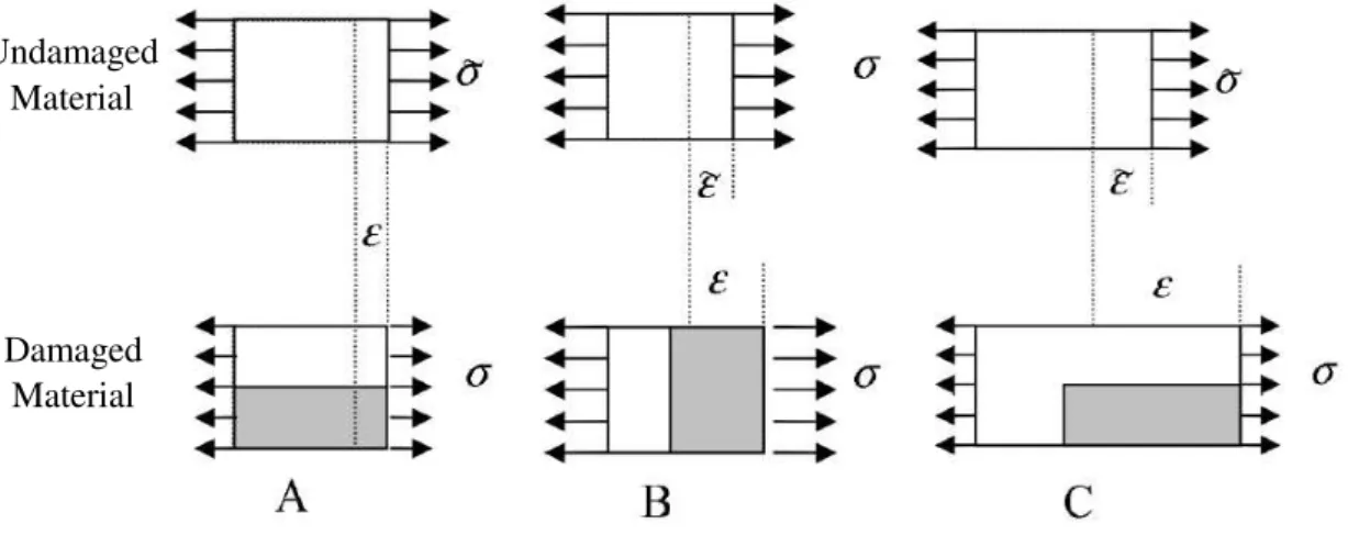
31 material. The stresses and strains in the effective space (of the undamaged material) follow the initial elastic law (𝜎̃ = 𝐶₀: 𝜀̃). In physical space, nominal stresses and strains are obtained by defining a relation between them and the effective stresses and strains.

Figure 2.15 presents the three main principles that can be followed to define those relations:

Figure 2.15 - “Hypothesis of A) strain equivalence, B) stress equivalence and C) energy equivalence

between the damage physical space and undamaged effective space”[18],[17]

Strain equivalence principal

The effective stress applied to the undamaged material (𝜎̃) causes the same strains that the nominal stress applied to the damage material. This results in a relation between the nominal stress (𝜎) and the effective stress (𝜎̃):

𝜎 = (𝐼 − 𝐷): 𝜎̃ 𝜎 = (𝐼 − 𝐷): 𝐶0: 𝜀

(54)

Stress equivalence principle

The effective strain (𝜀̃) applied to the undamaged material causes the same stresses that the nominal strain applied to the damage material (𝜀). This results in a relation between the nominal strains (𝜀) and the effective strains (𝜀̃):

𝜀̃ = (𝐼 − 𝐷): 𝜀 𝜎 = 𝐶0: (𝐼 − 𝐷): 𝜀

(55) Undamaged

Material

32

Energy equivalence principle

Helmholtz free energy density (Ψ) stored in the undamaged material under an effective strain is equal to the free energy density stored in the damaged material under a normal strain. At the same time, the complementary energy density stored in the undamaged material under an effective stress is equal to the complementary energy density stored in the damage material under a nominal stress.

Ψ =1_{2 𝜀̃: 𝐶}0: 𝜀̃

𝐺̅ =1

2 𝜎̃: 𝐶0−1: 𝜎̃ = 1

2 𝜎: 𝐶0−1: 𝜎

(56)

Resulting in:

𝜎 = (𝐼 − 𝐷): 𝐶0: (𝐼 − 𝐷)𝜀 (57)

2.3.2.

Macro-scale models

The propose of this models is to analyze the response of large structures [36]. At this level, the whole structure is considered homogeneous and continuum and the behavior of the material follows an anisotropic constitutive law [33].

Some macro-scale composite materials models are available in commercial finite element codes and rely on classical laminate plate theory. These models need a set of effective material parameters that can be obtained by meso-scale models and appropriate experimental tests [36].