ISSN 0104-530X (Print) ISSN 1806-9649 (Online)
Resumo: A globalização tem sido responsável pela elevação da exposição de empresas e países a riscos relativos a fatores cambiais. A literatura tem abordado a questão da volatilidade da moeda em países emergentes e desenvolvidos sem um consenso sobre tal dinâmica, bem como são escassos os estudos que estimam e situam o risco do real brasileiro. Dessa forma, o presente estudo teve por objetivo mensurar o risco da taxa de câmbio brasileira, bem como testar a hipótese de que existe uma diferença significante na volatilidade entre moedas de países emergentes e em desenvolvimento. Por meio do VaR paramétrico ajustado para distribuições de valores extremos, observou-se que o real brasileiro apresentou taxa de câmbio de maior risco. Os resultados também revelam que os pressupostos distribucionais não parecem apresentar nenhum padrão específico quando confrontados países emergentes e desenvolvidos, e também que países emergentes apresentaram menor volatilidade, denotando a preponderância de fatores externos ao mercado cambial na determinação do risco de algumas moedas.
Palavras-chave: Value-at-Risk; Taxa de câmbio; Risk Management; Países desenvolvidos e emergentes. Abstract: Globalization has been responsible for increasing exposure to risks related to currency factors for companies and countries. The literature has addressed the issue of currency volatility in emerging and developed countries without a consensus on such a dynamic and there are few studies that estimate and place the risk of the Brazilian real. Thus, this study aimed to measure the risk of the Brazilian exchange rate, as well as test the hypothesis that there is a significant difference in volatility between currencies of emerging and developing countries. Through the parametric VaR set to extreme values distributions, it was observed that the Brazilian real presented at greater risk of exchange rate. The results also showed that the distributional assumptions do not seem to have any specific pattern when faced emerging and developed countries and also emerging countries showed less volatility, reflecting the preponderance of factors external to the foreign exchange market in determining the risk of some currencies. Keywords: Value-at-Risk; Exchange rate; Risk management; Developing and emerging countries.
Value-at-Risk (VaR) Brazilian Real and currencies of
emerging and developing markets
Value-at-Risk (VaR) Real brasileiro e moedas de mercados emergentes e em desenvolvimento
Marina Andreotti Ogawa1
Naijela Janaina da Costa1
Herick Fernando Moralles1
1 Departamento de Engenharia de Produção, Universidade Federal de São Carlos – UFSCar, Rod. Washington Luís, Km 235, CEP 13565-905,
São Carlos, SP, Brasil. E-mail: [email protected]; [email protected]; [email protected] Received June 3, 2016 - Accepted Dec. 28, 2016
Financial support: None.
1 Introduction
The growth of the importance of risk management
lies in the volatility of financial variables, among
them, we can highlight the exchange rate, interest rate, capital market, and commodity prices. Factors such
as the end of fixed exchange rates, interest rate swings, financial crises, and sudden changes in
commodity prices contribute to the increase in market unpredictability (Jorion, 1997).
The exchange rate risk can be defined according
to Madura (1989) as the unexpected changes in the exchange rate, leading to direct losses (derived from
unhedged exposure), or indirect in the cash flows
(Papaionnou, 2006).
Managing exchange rate risk is related to a company’s decisions about its exposure to foreign currencies, according to Allayannis et al., (2001) and to manage it, it is crucial to understand the types of risks that are associated with the rate such as: transaction risks
(related to cash flow risk); translation risks relating
in order to manage the risk related to the exchange rate (Papaionnou, 2006).
After consecutive years of economic instability
and increasing inflation, Brazil underwent a process
of monetary and exchange rate reform in 1994, during which time the real plan was instituted, and since then
the Brazilian real has become the official currency
of Brazil (Batista, 1996). Thus, the real consists of
a floating exchange rate regime (more specifically a dirty float), that is, a regime that allows the existence
of appreciations and depreciation of the currency, leading to exchange rate volatility (Lara, 2005).
Volatility is a significant input parameter in the approach to options, both financial and real assets
(Oliveira & Pamplona, 2012).
According to Carvalho & Sicsú (2004), the high exchange rate volatility causes an increase in
uncertainties, reducing the predictability of financial costs. In this way, it can be inferred that significant devaluations in the local currency can benefit exporting
companies, while generating losses to those that present large amounts of debt in foreign currencies.
Thus, the risk of exchange rate fluctuations has a
strong impact on the economy and the performance of exporting industries. It is important to know and measure the risk related to the value of the currency (Akhtekhane & Mohammadi, 2012). In addition, the
currency can be considered as a financial asset like any other, being subject to fluctuations of supply and
demand, as well as speculative attacks.
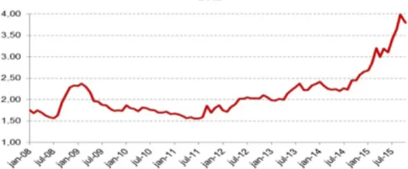
Therefore, the above factors are highlighted and based on the analysis of the current economic situation in Brazil, in which, in 2014, the dollar increased 13% in relation to the real and the real continues to show strong volatility in the year 2015. From this
it is important to measure the risk of this financial
variable (Federowski, 2015). The Figure 1 shows the evolution of the real against the dollar.
Despite the plurality of articles that use VaR to
measure the risk of different exchange rates, such
as Zhan & Tian (2000), Wang et al. (2010), Li et al. (2007), among others, there are few studies that investigate the exchange rate risk of the brazilian real. Moreover, in the current scenario, in which the country has been facing several economic and political reforms in which the local currency has been showing strong volatility, the measurement of the risk of the real acquires a character of urgency, presenting, therefore, great importance.
Wang et al. (2010) uses EVT (Extreme Value Theory) to estimate the tails of the yuan exchange
rate returns, finding high adherence to the Pareto
distribution. Although the VaR EVT underestimates the risk to the proposed exchange rate, such an approach still appears to be superior to the traditional
VaR calculation, such as historical simulation and variance-covariance.
The lack of consensus on distributional assumptions and VaR computation methods becomes more pronounced when compared to distinct economic realities, such as assets of developed economies and assets of emerging economies.
In fact, Gençay & Selçuk (2004) still argue that developing economies are much more subject to change in the short term, and therefore, the probability distributions of their returns and estimated parameters are also likely to change with some frequency. In addition, developing markets are more subject to
financial swings.
Kittiakarasakun & Tse (2011) argue that financial
models are often not applicable to emerging markets as well as developed markets, for example, G7. This could occur because, often, developing countries
impose restrictions on the free flow of capital. The difference in markets is reflected in the tails of
probability distributions of returns, which especially for emerging markets, tend to be non-normal. In fact,
Longin (2005) argues that distribution tails are different
in emerging markets.
However, Kittiakarasakun & Tse (2011) also argue
that the differences between Asian and US returns
may be merely a matter of scale, since the occurrence of extreme events in Asia is as likely as in the United States, demonstrating that market tails chinese and the north american market are similar. This denotes that a risk management model would work well for
both realities. This fact is verified, since the study conducted by the authors did not find significant differences in the risks measured by VaR.
Thus, risk measurement has been a major concern among managers and regulators, with Value-at-Risk (VaR) being one of the most commonly used tools for risk measurement.
According to Jorion (1997), VaR is a risk measurement method that uses standard statistical techniques, in other words, VaR measures the worst loss expected over a given time interval within a
given confidence level.
2
Value-at-Risk
The problem of measuring and controlling financial
risk has motivated researchers and decision makers to seek indicators capable of identifying how risky a decision is (Ribeiro & Ferreira, 2005).
Value-at-Risk (VaR) is one of the most popular
risk measurement tools used by the financial sector. It was created in the 1990s, shortly after the financial
disasters such as that of Barings, cited above, and can
be defined as the maximum expected loss of a portfolio, with a certain level of significance α (or confidence level 1-α) in a given time horizon (Moralles et al.,
2013, Aragón et al., 2013). For example, if we have
a daily VaR of R $ 1 million with a confidence level
of 99%, there is only 1% chance of a loss being more than R $ 1 million on any business day.
In this way, the VaR provides an indication of the probability of a potential change in the value of a portfolio resulting from the change in market conditions over a given period of time by demonstrating how likely the VaR measure can be exceeded (Crouhy et al., 2006).
Gaio & Pimenta (2012) point out that VaR is one of the most important market risk measurement tools and, undoubtedly, the one most used by institutions and risk managers. Estimating the maximum expected loss, within a period of time and a given level of
confidence, one has the known market risk.
2.1 Exchange rate regimes
According to Zini (1996), the legal regime refers to the set of characteristics derived from norms, laws and practices that regulate transactions with foreign currencies in the economy. In economic terms, the exchange rate regime consists of the way a country’s exchange rate is determined, that is, whether the
exchange rate is fixed, fluctuating or assuming some
variation between these two (intermediate regimes). When a country adopts an exchange rate regime, it expects it to assist in economic stability, stimulate foreign trade and investment, provide conditions for
fiscal and monetary policy management, and protect
the domestic economy from disruptions arising from
international finance (Sambatti & Rissato, 2004). In the fixed exchange regime, the nominal exchange rate is fixed and parity must be maintained through the
intervention of the Central Bank in the foreign exchange market, buying or selling currency according to the adjustment needs of that market. If there is excess supply (demand) of foreign exchange, the Central Bank intervenes in the market by buying (selling)
currencies at the fixed rate. Thus, the credibility of
this system depends on the capacity of intervention of the Central Bank, via available international reserves (Zini, 1996).
Like this, the fixed exchange rate regime tends to
provide more stable horizons to the exchange rate, since Thus, it is observed that the VaR is an easy-to-understand
method capable of providing benefits such as the provision of management information, performance evaluation, as well as contributing to resource allocation decisions, thus constituting one of the most important tools for Risk management (Jorion, 1997).
The literature about VaR is quite extensive and has important works such as Chela et al. (2011), Gaglianone et al. (2008), Jorion (2007), Taylor (2005), Glasserman et al. (2000), so that there are several ways to estimate VaR, among them, nonparametric methods (historical simulation), parametric (variance covariance method), simulation (Monte Carlo method), and conditional heteroscedasticity methods, in particular, the GARCH models (Wang et al., 2010). Since the use of VaR is of interest in addition to companies
and financial institutions, regulatory agencies have
also been underestimating their importance so that, since 1988 with the Basle Accord, several regulatory initiatives involving VaR (Jorion, 1997).
However, although there is no consensus on which probability distributions to use, and the weaknesses of parametric VaR under normality assumptions, parametric VaR is extremely interesting because of its
simplicity of calculation and efficacy when correctly
specifying the distribution of returns. And should therefore be abandoned as an alternative to the VaR computation (Moralles et al., 2013).
In view of the above, the main objective of this paper is to measure the risk of the Brazilian exchange rate, as well as to test the hypothesis that there is
a significant difference in the volatility between
currencies of emerging and developing countries, as stated by authors such as Kittiakarasakun & Tse (2011), Longin (2005) and Gençay & Selçuk (2004).
In view of the above, the main objective of this paper is to measure the risk of the Brazilian exchange rate, as well as to test the hypothesis that there is
a significant difference in the volatility between
currencies of emerging and developing countries, as stated by authors such as Kittiakarasakun & Tse (2011), Longin (2005) and Gençay & Selçuk (2004). Thus, the study will compare the risk of currencies
from different countries, separated into two groups, emerging and developed. The first group consists
Convertible currencies are those that are freely accepted by other countries, without any restriction and in any market, known as Strong Currency. Nonconversible currencies are those that do not have an easy international course or that are not accepted by other countries in foreign exchange transactions. Chart 1 shows the main examples of convertible and inconvertible currencies.
2.1 Foreign exchange risk
The fixed exchange rate regime was widely used
until the mid-1980, however, with improved markets, high capital mobility, this type of regime was losing
strength and fans, and today most countries use floating
exchange rate regimes (Lara, 2005).
The fixed exchange regime is a system in which the Central Bank of a country establishes a fixed
value for the parity between the local currency and the dollar.
The floating exchange rate regime allows the
currency to appreciate and depreciate, which causes exchange rate volatility (Lara, 2005). This type of
scheme was introduced for the first time in 1973, and
since its introduction, the exchange rates of several currencies have a much more volatile behavior than the factors governing their behavior, such as domestic and international money supply, Prices, and the international balance of payments (Lintz, 2004). This feature emphasizes the importance of
understanding these fluctuations and managing the risk of this financial variable.
The exchange rate concept consists of the reference value of a currency in relation to a second currency. Therefore, an increase in the exchange rate means the devaluation of the currency in question against the reference. The opposite is true.
According to Madura (1989) exchange rate risk
is related to the effects of unpredicted exchange
rate changes on contracts involving more than one currency, that is, their recurring obligations and rights. it assists in the stability of prices and expectations,
serving as a reference in the decision-making of the agents and thus allowing the increase of trade and
Investments. Thus, by fixing the exchange rate, the
risk of uncertainties caused by high exchange rate variability tends to be eliminated (Frankel, 1999).
The pure floating exchange rate regime is one in
which the Central Bank does not intervene in the foreign exchange market. The exchange rate is determined by the supply and demand of foreign currency. In this way, the Central Bank is free to maintain high levels of international reserves (Zini, 1996; Corden, 2001).
However, the configuration of this regime is more
evident in theory than in practice, since, normally,
what is verified is some degree of exchange monitoring
in the form of direct intervention in the exchange market, by the Central Bank, in order to avoid movements of high volatility, in the short run, which may compromise certain economic policy objectives,
in practice, a regime of managed fluctuation known as dirty flotation. In this case, the Central Bank does not advocate a specific exchange rate, but it intervenes
in the exchange market (Corden, 2001).
As a result of the great exchange rate volatility
observed after 1973, along with the difficulties
encountered in maintaining monetary stability in a
context of financial liberalization, especially in the
1980s, discussions on exchange rate regimes, according to Edwards & Savastano (1999) started to incorporate the intermediate regimes, standing out among them:
the one of exchange bands; the floating flotation, the crawling peg; the fixed but adjustable exchange rate;
the currency board and the full dollarization. Each of these regimes has characteristics that bring them closer to one or the other of the canonical regimes.
2.2 Convertibility
As a natural consequence of acceptability at the international level, one has the characteristic of currency convertibility. The currencies, under the
exchange rate aspect, are classified as: convertibles;
and, inconvertible.
Chart 1. Convertible and inconvertible currencies.
Convertible Currencies Non-convertible currencies
US Dollar (USD) Chilean Peso (CLP)
Canadian Dollar (CAD) Indian Rupee (INR)
Australian Dollar (AUS) Argentine Peso (ARG)
Pound Sterling (GBP) Real (BRL)
Swiss Franc (CHF) New Peruvian Sol (PEN)
Japanese Yen (JPY) Mexican Peso (MXN)
Euro (EUR) Chinese Yuan (CNY)
Danish Kroner (DKK) South Korean Won (KRW)
time in a year. Growing doubt about central banks’
ability to generate growth and inflation in Japan and
Europe and the optimism that emerging countries will avoid a generalized economic slowdown have
affected exchange rate patterns (África21, 2016).
Currency gains due to weakening dollar are not welcome in developed countries struggling to boost economic growth, but on the other hand are well received by central banks of emerging market countries, which
fight capital outflows and Depreciations. The outlook
for emerging markets has also improved since concerns about China’s growth slowed, and the recovery in commodity prices boosted revenues for producers
such as South Africa or Brazil (África21, 2016), as China adopts a fixed exchange rate in relation to the
US dollar and, like Russia, uses the currency anchor.
3 Research method
The present research has interests focused mainly on the measurement of risk in the local currency (real) to compare it with other currencies, in order to position the volatility of the real against other currencies, as well as verify the hypothesis that developing economies have More volatile currencies. This work starts from the calculation of the parametric
VaR adjusted for different theoretical probability
distributions according to the Kolmogorov-Smirnov and Anderson-Darling adhesion tests for the extreme values of Moralles et al. (2013).
The US dollar (USD) was the currency selected as the reference currency, since it is the currency most used in international transactions, as well as being used as an international reserve worldwide. Given the above, the historical series of the Brazilian real (BRL) and other twelve currencies were collected, based on their value against the dollar. Sampling will be divided into two groups: emerging and developed
countries. The first group consists of: Argentine
peso (ARG); Chilean peso (CLP); New Peruvian sun (PEN); Mexican peso (MXN); Chinese yuan (CNY); Indian Rupee (INR); And, won South Korean (KRW). The second group consists of: Australian dollar (AUS); Euro (EUR); Swiss Franc (CHF); Pound sterling (GBP); And, Japanese Yen (JPY). Such sampling was chosen to compare the proposed VaR calculation method between developing markets, developed markets and the Asian market.
For the accomplishment of the experiment, the daily quotation of the currencies shown in Chart 3 and the quotation of the brazilian currency between the years of 2008 and november 9, 2015 through the website of the Central Bank of Brazil were collected. The choice of this time horizon seeks to encompass According to Jorion (1997) the VaR can be used
to determine the exposure of financial risks such as
the exposure to currencies, that is, exchange rate risk. For such, one can use the three methods described above, and their returns are calculated from the
difference between the daily quotation of one currency
against the other, and the dollar is used for the most part as a reference (Papaionnou, 2006).
For example, papers such as Papaionnou (2006) calculate the exchange rate risk for companies. Wang et al. (2010) estimates the risk of the Chinese yuan through the use of VaR based on extreme value. The work of Zhan & Tian (2000) measures the risk in the Japanese yen. While Li et al. (2007) propose a model to estimate the VaR of a portfolio of Canadian dollars and Japanese Yen. Akhtekhane & Mohammadi (2012) calculate the Rial-Euro VaR using the parametric method and the historical (non-parametric) simulation method. It is possible
to find other articles and researches that approach
the theme.
2.2 Volatility between currencies of emerging and developing countries
The First World represents developed countries, with great potential in the industrial area, in structured policy and high Human Development Index, such as: Norway, United States, Sweden, Japan, Germany, France, and Italy.
No rules are defined regarding the classification of
developed, emerging and underdeveloped countries. It is based on market statistics. Those located in the central area of Asia, according to the United
Nations, do not fall under any of these classifications.
They are: Kazakhstan, Uzbekistan, Kyrgyzstan, Tajikistan and Turkmenistan. Nor is Mongolia in the class. These countries are in another category, that of countries in transition. However, they are related in conjunction with developmental ones.
It is worth mentioning the G7 or Group of Seven that it is a forum composed of seven nations that together represent half the world economy. It is comprised of Germany, Canada, the United States, France, Italy, Japan and the United Kingdom.
The exchange rate represents an important element to be considered for the growth trajectory in developed and emerging nations, underlining the
effects of the exchange rate volatility of exchange rate regimes in inflationary contexts on the growth
of the latter (Araújo, 2009). The Chart 2 represents some authors who studied the real exchange rate and economic performance.
The implied volatility of developed country
Chart 2. Authors who studied the real exchange rate and economic performance.
Author(s)/Population of
study/Sample Objectives/Results found
Damiani (2008)/26 countries, 13 emerging and 13
developed/(1971-2006)
This paper aims to discuss the exchange rate relationship with economic growth for emerging countries compared to developed countries. The empirical results found in this paper support the importance of the exchange rate as a relevant element to be considered for growth trajectory, for rich and emerging countries, underlining the effects of the exchange rate volatility of exchange rate regimes in inflationary contexts on the growth of the latter. The article presents the results generated by a dynamic panel that tested the relationship of economic growth with the exchange rate volatility and the choice of the exchange regime of 26 countries. The results of the emerging countries suggest a greater vulnerability to exchange rate volatility, as well as a greater relevance to the exchange rate regime adopted. For the developed ones, only the choice of regimes is relevant; However, in a considerably more attenuated way.
Araújo (2009)/90 emerging countries/(1980-2007)
The author investigated the relationship between economic growth and exchange rate volatility in emerging and developing countries. It was estimated a model that relates the economic growth to the exchange rate volatility in a data panel. The estimates indicated a negative and highly significant impact of exchange rate volatility on economic growth, confirming the theoretical prediction that exchange rate instability has negative effects on the real economy. Estimates have shown that exchange rate volatility has a negative and significant effect on economic growth in the countries studied, suggesting that these countries would benefit from policies that would contribute to greater stability of their exchange rates.
Schnabl (2007)/41 countries on the periphery of the European Monetary Union/ (1994-2005)
The author studied the real exchange rate and economic performance, and as results the estimates revealed an inverse and statistically significant relationship between exchange rate volatility and economic growth in developing countries with financial openness. For the group of European non-monetary European industrialized countries the benefits of stable exchange rates appeared to be weaker. This may be due to the fact that the more developed capital markets have made them less vulnerable to exchange rate variation.
Aghion et al. (2009)/83 countries/(1960-2001)
The empirical results indicated that real exchange rate volatility has a negative impact on long-term productivity growth, and the effect depends critically on the level of financial development. The results showed robust for time window, alternative measures of financial development and exchange rate volatility and discrepant values.
Kittiakarasakun & Tse (2011)/Return on equity indexes in Asia/(1989-2009)
The authors analyzed whether stock returns in Asian markets are characterized by infinite variance or by large variation, which has an important implication for the applicability of many financial models to Asian market data. The Value-at-Risk method was applied using Asian and North American data and no significant difference in performance was found. The Extreme Values Theory (TVE) was also applied to characterize the return distributions of the stock indices. The authors noted that Asian stock markets are more volatile than developed markets, but the occurrence of extreme price changes is as likely in Asian markets as in developed markets.
Bekaert & Harvey (2000)/17 countries/(1977-1996)
The objective of this study was to identify breaks in the capital flows of seventeen countries. Of these, sixteen are interrupted by an increase in net capital flows. In some countries, it appears that the flows of securities precede capital flows. It was analyzed that the expected returns decrease after significant decreases in capital flows. In addition, the risk decreases, at least as measured by the country’s rating, and the correlations of capital returns with the world market is larger. It was analyzed that the increase in capital flows is associated with a lower cost of capital, higher correlation with world market returns, lower concentration of assets, lower inflation, larger market size in relation to GDP, more trade, and slightly Higher per capita economic growth.
Source: Prepared by the authors (2016).
the period of financial crises beginning in 2008 and
the current volatility of the brazilian currency. Then, from the daily closing value of each currency against the Real, the daily returns were calculated through Equation 1.
1 ln ln
t t t
R = r− r− (1)
If
1
KS≤K−α, which K1−α are values critical to a significance α. And,
Additionally, ϕi it is specified by (4),
1 1
2
(2 1)[ln( ) ln(1 )]
n
i n i
i
i
A n
n
ϕ ϕ + −
= − − + −
=
∑
− (4)Which, ϕi is a given probability distribution
If, 2 1
A ≤A−α
Which, A1−α are values to a significance α for a distribution ϕi.
Once the distributions that best represent the series were obtained, the calculation of the daily VaR, obtained from the same software, was performed at
a significance level of 50% for the composite series
of the 10% lower values, in order to obtain a Level
of significance of 5% for the whole series.
In these terms, the model presented for the VaR calculation will be (Equation 5).
[ ]
1
( ) i ( | , , ) : ( | , ,
VaR x =ϕ− p µ σ ξ = x ϕ x µ σ ξ (5)
Which,
p is the level of significance used for the VaR calculation.
, ,
µ σ ξ are respectively parameters of mean, standard deviation, and distribution format ϕi using iterative
numerical methods. 1( )
i x
ϕ− is the inverse cumulative density function of
the probability distribution to be specified by the goodness-of-fit tests.
Finally, to validate the VaR calculation method, backtesting was performed (Kupiec 1995), which calculates the interval for VaR acceptance given by the likelihood ratio of a Bernoulli distribution of (Equation 6).
2 ln[(1 )T N n] 2 ln[(1 ( / ))T N( / ) ]N
L= − −p − p + − N T − N T (6)
Whose interval limit is given by (Equation 7),
2 (1)
2 ln( )L −2 ln( 0) ~L χ (7)
Thus, the inerval created by the Kupiec test allows one to evaluate if the estimated VaR is under control, that it, to verify if it is not underestimated or overestimated.
4 Results
Regarding the evolution of the Brazilian real against the dollar at the end of each month between january 2008 and november 2015, it is stated that the currency
suffered a strong devaluation in the recent period, with
the Real depreciating by 49.4% In the last 12 months, that do not admit negative values, Equation 1 was
calculated in logarithmic terms in order to maintain percentage proportionality, but using terms in positive values (Moralles et al., 2013), as shown in Equation 2.
t
R p
R =e (2)
Rp are the returns expressed in exponential terms from the returns Rt obtained in Equation 2. Once this has been done, the accumulated empirical probability distribution of the various currencies will be assembled, representing their return. In order to better parameterize the empirical distribution, as well as to capture the extreme values of the left tail, and consequently to obtain a VaR that best represents reality, the extreme value theory (EVT) will be applied, reducing the importance of the central values and the right tail. It is better to predict the movements related to the extreme values that consist of the method developed by Moralles et al. (2013).
In this way, a second series will be constructed for each coin, and this new series will be composed by the 10% lower returns found during the studied period. Thus, this work aims to apply extreme value theory (EVT) in order not to overestimate or underestimate risk exposure. Being that, when working with the extreme values, a probabilistic distribution is obtained that better adheres to the left tail, which will result in a more realistic VaR.
Subsequently, these distributions will be compared with other theoretical distributions. Then, the Kolmogorov-Smirnov adhesion test and the Anderson-Darling adhesion test will be used, which will indicate the degree of agreement between the sample distribution and the theoretical distribution (Moralles et al., 2013). The Kolmogorov-Smirnov and Anderson-Darling adhesion test was performed from a routine developed by EasyFit 5.6.
Thus, the distribution to be used in the VaR calculation will be based on (Equation 3).
maxx n( ) ( )
KS= F x −F x (3)
Chart 3. Exchange rates used.
Group 1 - Emerging Group 2 - Developed
ARG/USD EUR/USD CLP/USD CHF/USD MXN/USD GBP/USD PEN/USD AUS/USD CNY/USD JPY/USD INR/USD KRW/USD BRL/USD
United Kingdom and Australia. Finally, in Figure 4, it is possible to observe the behavior of the currencies of Japan, South Korea, China and India.
Note that for the great majority of currencies there
were more pronounced fluctuations during periods
of crisis, especially in the second half of 2008 and beginning of 2009, when volatility spikes are more pronounced. It is also possible to observe that, for more recent dates, the graphs show a greater volatility when compared to previous periods, although it is less marked than that between 2008 and 2009.
In view of this volatility presented in all currencies studied, it is possible to emphasize again the need reaching its maximum price of R$ 4.21 during the
study period on September 29, 2015. Moreover, the currency was very volatile between 2008 and 2009. It is important to note that both in 2008 and 2009 Brazil has experienced economic crises, and today the country is experiencing a strong economic
recession, which justifies the volatility presented by
the currency during the periods highlighted. In the graphs shown in Figure 2, prices are shown at the end of each month in each of the Latin American countries - Argentina, Chile, Mexico and Peru. Figure 3 shows the same observation for the currencies of the European Union, Switzerland, the
Figure 2. Evolution of the exchange rate of Latin American countries. Source: Prepared by the authors (2016).
of the same group, than when comparing currencies
of different groups.
The Chart 5 shows that the probability distribution
that best describes the series of returns of different
exchange rates for the Kolmogorov-Smirnov test consists of the general extreme value distribution (GEV), appearing ten times, whereas for The Anderson-Darling test, both GEV functions and power function appeared 3 times.
From the distributions obtained as well as the parameters of each distribution, it was possible to calculate the VaR of the real and other currencies.
The average daily VaR of the real equals -1.45%, ie on a business day, there is only 5% probability of the actual loss being greater than 1.45%. Mean VaR was obtained by averaging the VaR calculated by the Kolmogorov-Smirnov test and the Anderson-Darling test. The results obtained can be seen in Chart 6. and importance in measuring and knowing the risks
involved in exchange rates.
Once the returns for each coin were obtained, the adhesion test was performed for the lowest 10% values of each distribution, in order to obtain the probability distribution that best portrayed the left tail of each series.
The results obtained by the adhesion test performed by the software EasyFit 5.6 are shown in Charts 4 and 5.
The Chart 4 shows that different distributions for the same series, with the exception of the Chilean peso, of the Canadian dollar and the Indian rupee
were obtained for the different test types, in which
both tests resulted in the adherence of one Same distribution - General Extreme Value (GEV). Moreover, it is notorious that coins of the same group exhibited relatively similar behavior. As the similarities are more recurrent in the comparison between currencies
Chart 4. Result of the adhesion test.
Adherence tests
Kolmogorov-Smirnov Anderson-Darling
Group 1
ARG/USD Gen. Extreme Value Johnson SB
CLP/USD Gen. Extreme Value Gen. Extreme Value
MXN/USD Gen. Extreme Value Power Function
PEN/USD Gen. Extreme Value Log-Pearson 3
JPY/USD Power Function Power Function
Group 2
EUR/USD Gen. Extreme Value Kumaraswammy
GBP/USD Power Function Dagum
CHF/USD Dagum Weibull (3P)
CAD/USD Gen. Extreme Value Gen. Extreme Value
CNY/USD Gen. Extreme Value Power Function
INR/USD Gen. Extreme Value Gen. Extreme Value
KRW/USD Gen. Extreme Value Kumarasw amy
Source: Prepared by the authors (2016).
Before analyzing the observed results, the backtesting was performed, in order to verify if the method proposed for the VaR calculation presented acceptable VaR values. The results obtained in the backtesting step can be observed in Chart 7. It can be observed that the proposed method presented acceptable results, within the
confidence interval. There was only one observation
outside the acceptable region, which consisted of the VaR calculated by Anderson-Darling for the South Korean Won. That is, in general, the proposed method - calculation of the VaR by the parametric method through the test of adherence to extreme values - points VaR values that do not overestimate or underestimate the risk.
The Chart 8 shows the results in descending order in absolute terms for each type of test, while Chart 9 shows the mean VaR values in descending order.
From the previous charts, it is observed that the Real presents the highest risk among all currencies studied, with only the Australian dollar surpassing the risk of the Real in the Kolmogorov-Smirnov test. In addition, it is possible to note that the currencies of the emerging countries have the lowest risk, with an average VaR of -0.78% and a median of -0.78%.
However, the low value of the group’s average VaR can be explained by the fact that the Argentine currency presents a very small risk, with a VaR of
-0.16%, which can be justified by the presence of
an interventionist government that Does not allow
the currency to float freely in the market. This fact
can also be observed in Figure 2, where it is noticed that, although the currency has devalued over time, it consisted of a regular and constant devaluation. By including the Real in the average of the emerging group, the VaR rises to -0.78% (Chart 10).
In absolute terms, the developed group had an average VaR equal to -1.15%, 37% above the VaR Chart 5. Frequency of adhesion test results.
Adherence tests
Kolmogorov – Smirnov Anderson-Darling
Distribution
Gen. Extreme Value 10 3
Power Function 2 3
Dagum 1 2
Kumarasw amy 0 2
Johnson SB 0 1
Log-Pearson 3 0 1
Weibull (3P) 0 1
Source: Prepared by the authors (2016).
of the emergent group. It is worth noting that the low risk observed in the Chinese currency is due to the presence of a strong and interventionist government that, together with the high international reserves, controls the exchange rate variation of the currency according to its internal policies. Thus, group 2 (developed) showed to be the group with a riskier exchange rate. As can be seen in Chart 10.
Given the above, it can be inferred that the Brazilian currency presents a divergent behavior of the currencies studied. Its risk was closer to the Australian dollar, whose VaR is 1.22% lower than the Real VaR (Chart 11). The high risk presented by the Brazilian currency can be explained by the current political and economic crisis that the country is going through, being a crisis almost exclusive of the country, so the volatility of the period is much higher than the others, which increases its risk.
Chart 6. VaR by Currency Group.
Kolmogorov-Smirnov % Anderson-Darling % VaR Médio %
Group 1
BRL -1.41 -1.50 -1.45
ARG -0.16 -0.16 -0.16
CLP -1.08 -1.08 -1.08
MXN -1.04 -1.12 -1.08
PEN -0.47 -0.48 -0.47
CNY -0.17 -0.18 -0.17
INR -0.75 -0.75 -0.75
KRW -0.99 -1.16 -1.07
Média -0.76 -0.80 -0.78
Mediana -0.76 -0.80 -0.78
Group 2
EUR -1.07 -1.10 -1.08
GBP -0.95 -0.98 -0.97
CHF -1.15 -1.24 -1.19
AUS -1.43 -1.45 -1.44
JPY -1.08 -1.08 -1.08
Média -1.14 -1.17 -1.15
Mediana -1.08 -1.10 -1.08
Source: Prepared by the authors (2016).
Chart 7.Backtesting.
Número de superações
Currency Sample Size Confidence Interval
Kolmogorov-Smirnov Anderson-Darling Average VaR
BRL 2048 81<T<125 99 90 94
ARG 2048 81<T<125 103 99 102
CLP 2048 81<T<125 111 111 111
MXN 2048 81<T<125 108 90 100
PEN 2048 81<T<125 101 101 101
EUR 2048 81<T<125 107 103 105
GBP 2048 81<T<125 104 98 102
CHF 2048 81<T<125 105 89 96
AUS 2048 81<T<125 94 92 93
JPY 2048 81<T<125 98 98 98
CNY 2048 81<T<125 103 97 100
INR 2048 81<T<125 101 101 101
KRW 2048 81<T<125 104 77 90
Source: Prepared by the authors (2016).
Chart 8. VaR in ascending order by adherence test.
Anderson-Darling % Kolmogorov-Smirnov %
BRL -1.50 AUS -1.43
AUS -1.45 BRL -1.41
CHF -1.24 CHF -1.15
KRW -1.16 CLP -1.08
MXN -1.12 JPY -1.08
EUR -1.10 EUR -1.07
CLP -1.08 MXN -1.04
JPY -1.08 KRW -0.99
GBP -0.98 GBP -0.95
INR -0.75 INR 0.75
PEN -0.48 PEN -0.47
CNY -0.18 CNY -0.17
ARG -0.16 ARG -0.16
5 Conclusions
The exchange rate is a fundamental variable in the process of economic development. Being that it composes one of the pillars of the Brazilian economy. Given its importance, the focus of this paper was to understand the volatility of the Brazilian currency in comparison with currencies of other countries, in order to establish a relationship between them by calculating Value-at-Risk (VaR).
The currencies studied were divided into two groups: currencies of emerging countries; and, currencies of
developed countries. The first group consisted of:
real (BRL); Argentine peso (ARG); Chilean peso (CLP); New Peruvian sun (PEN); Mexican peso (MXN); Chinese yuan (CNY); Indian Rupee (INR); and, won South Korean (KRW). The second group consisted of: Australian dollar (AUS); Euro (EUR); Swiss Franc (CHF); Pound sterling (GBP); And, Japanese Yen (JPY). Such sampling was chosen to compare the proposed VaR calculation method between developing markets, developed markets and the Asian market.
It should also be noted that the currencies of the developed countries are convertible currencies, that Chart 9. Average VaR in descending order.
Kolmogorov-Smirnov % Anderson-Darling VaR Médio %
BRL -1.41 -1.50 -1.45
AUS -1.43 -1.45 -1.44
CHF -1.15 -1.24 -1.19
EUR -1.07 -1.10 -1.08
CLP -1.08 -1.08 -1.08
JPY -1.08 -1.08 -1.08
MXN -1.04 -1.12 -1.08
KRW -0.99 -1.16 -1.07
GBP -0.95 -0.98 -0.97
INR -0.75 -0.75 -0.75
PEN -0.47 -0.48 -0.47
CNY -0.17 -0.18 -0.17
ARG -0.16 -0.16 -0.16
Source: Prepared by the authors (2016).
Chart 10. Mean VaR.
Average % Medium
Group 1 -0.68 -0.72
Group 2 -1.15 -1.08
Group 1 + BRL -0.78 -0.78
Source: Prepared by the authors (2016).
Chart 11. Variation of VaR in relation to Real VaR.
VaR Middle Absolute Terms % Variation in relation to the Real %
BRL 1.45 0.00
AUS 1.44 -1.22
CHF 1.19 -17.94
EUR 1.08 -25.59
CLP 1.08 -25.69
JPY 1.08 -25.69
MXN 1.08 -26.01
KRW 1.07 -26.28
GBP 0.97 -33.58
INR 0.75 -48.24
PEN 0.47 -67.58
CNY 0.17 -88.03
ARG 0.16 -89.23
is, they are freely accepted by other countries, without any restriction and in any market, since the currencies of the emerging countries are inconversible currencies, that is, they are Those currencies that do not have an easy international course or that are not accepted by other countries in foreign exchange transactions. Thus, this aspect was also considered as a parameter
of classification of the two groups.
For this, the VaR of each coin was calculated by the parametric method by applying the extreme value theory (EVT) in order to best represent the extreme values, and the Kolmogorov-Smirnov and Anderson-Darling adhesion tests were performed to
reflect more accurately the actual historical distribution,
resulting in a calculation method that proved to be
effective, since the results obtained were within the confidence interval proposed by the backtesting,
except for one sample. From this, it was possible to conclude that the average daily VaR of the real against the US dollar was -1,45%, a risk 65% higher than the average values obtained for the other twelve currencies studied. That is, the obtained VaR implies that there is only 5% probability in the real to incur a loss above 1,45% on a business day.
It was also observed that group 1 (emergent) had an average VaR of -0.78%, consisting of the lowest risk group, that is, the currencies of emerging countries presented a lower risk in relation to the US dollar among the groups studied. It is important to note that the argentine peso was the one that resulted in the lowest VaR equal to -0.16%, being, therefore, the less risky currency. Group 2 (developed) presented an average VaR of -1.15% and proved to be the group with the most risky exchange rates.
It is worth mentioning that in the period studied Argentina was in fact not very connected to international markets, which may explain the resistance of the peso to external shocks - that is, it is not only the degree of intervention that explains the paradoxical result of the performance of the argentine peso. The results showed that economies in similar stages and near maturity levels show a similar exchange rate behavior, so the results obtained for currencies of the same group were within the same range of values. The results showed that the Argentine peso (ARG) was the least risky currency in the period studied, followed by the Chinese yuan (CNY), the new Peruvian sol (PEN) and the Indian rupee (INR).
Thus, the findings of the present study are in
agreement with the one found by Schnabl (2007),
which verifies an inverse relationship and between
exchange rate volatility and economic growth in
developing countries with financial openness. Also, the
results presented contradict Damiani (2008), which states that emerging countries are more vulnerable to exchange rate volatility, since the calculated VaR lower are in the fashions of emerging nations.
And, following the same reasoning, the findings of
the present study contradict Araújo (2009), which states that exchange rate volatility has a negative
and significant effect on economic growth.
Therefore, in general terms, the volatility of currencies and their relation to development seem to be much more related to the level of government intervention on the value of currencies than with market factors described above. Thus, a mode with
totally fluctuating change, although more volatile, points to the efficiency of the regulatory mechanisms
of an exchange with low intervention. Regarding the predictability of the VaR methods, Kittiakarasakun & Tse (2011) and Gençay & Selçuk (2004) argue
that financial models are often not applicable to
both emerging and developed markets, as well
as the difference in markets reflected in the tails
of probability distributions of returns. However, the results presented show a high incidence of generalized extreme value distribution (VEG) by the Kolmogorov-Smirnov test; And a pattern indistinct by the Anderson-Darling test. Like this, in terms of VaR computation, distributional assumptions do not
seem to have any specific pattern when confronted
with emerging and developed countries, so it is not possible to say that developing country currencies are actually more volatile.
References
África21. (2016). Volatilidade de moedas deixa países emergentes e afeta desenvolvidos. Recuperado em 26 de maio de 2016, de http://www.africa21online.com/ artigo.php?a=20772&e=Economia
Aghion, P., Bacchetta, P., Ranciere, R., & Rogoff, K. (2009). Exchange rate volatility and productivity growth: the role of financial development. Journal of Monetary Economics, 56(4), 494-513. http://dx.doi.org/10.1016/j. jmoneco.2009.03.015.
Akhtekhane, S. S., & Mohammadi, P. (2012). Measuring exchange rate fluctuations risk using value-at-risk. Journal of Applied Finance & Banking, 2(3), 65-79.
Allayannis, G., Ihrig, J., & Weston, J. (2001). Exchange rate hedging: financials vs. operatonal strategies. American Economic Review Papers and Proceeding, 91(2), 391-395.
Aragón, C. S., Pamplona, E., & Vidal Medina, J. R. (2013). Identificação de investimentos em eficiência energética e sua avaliação de risco. Gestão & Produção, 20(3), 525-536. http://dx.doi.org/10.1590/S0104-530X2013000300003.
Risk. Management Science, 46(10), 1349-1364. http:// dx.doi.org/10.1287/mnsc.46.10.1349.12274.
Jorion, P. (1997). Value-at-risk: a nova fonte de referência para o controle do risco de mercado. São Paulo: Bolsa de Mercadorias & Futuros.
Jorion, P. (2007). Value-at-Risk: the new benchmark for managing financial risk (3rd ed.). New York: McGraw Hill. Kittiakarasakun, J., & Tse, Y. (2011). Modeling the fat
tails in Asian stock markets. International Review of Economics & Finance, 20(3), 430-440. http://dx.doi. org/10.1016/j.iref.2010.11.013.
Kupiec, P. H. (1995). Techniques for verifying the accuracy of risk management models. Journal of Derivatives, 3(2), 73-84. http://dx.doi.org/10.3905/jod.1995.407942.
Lara, L. R. (2005). Regimes Cambiais Alternativos para o Caso Brasileiro (pp. 1-16). Curitiba: PET-Economia. Recuperado em 26 de maio de 2016, de http://www. pet-economia.ufpr.br/banco_de_arquivos/00013_ RegimesCambiais.pdf
Li, S. P., Wang, H. L., & Li, D. (2007). External dependence model of foreign Exchange rate. Journal of System Engineering, 27, 82-86.
Lintz, A. C. (2004). Dinâmica de bolhas especulativas e finanças comportamentais:um estudo de caso aplicado ao mercado de câmbio brasileiro (Tese de doutorado). Faculdade de Economia, Administração e Contabilidade, Universidade de São Paulo, São Paulo.
Longin, F. (2005). The choice of the distribution of asset returns: How extreme value theory can help? Journal of Banking & Finance, 29(4), 1017-1035. http://dx.doi. org/10.1016/j.jbankfin.2004.08.011.
Madura, J. (1989). International Financial Management (2nd ed.). St. Paul, Minnesota: West Publishing Company.
Moralles, H. F., Rebelatto, D. A. N., & Sartoris, A. (2013). Parametric VaR with goodness-of-fit based on EDF statistics for extreme returns. Mathematical and Computer Modelling, 58(9-10), 1648-1658. http:// dx.doi.org/10.1016/j.mcm.2013.07.002.
Oliveira, R. J., & Pamplona, E. O. (2012). A volatilidade de projetos industriais para uso em análise de risco de investimentos. Gestão & Produção, 19(2), 337-345. http://dx.doi.org/10.1590/S0104-530X2012000200008.
Papaionnou, M. G. (2006). Exchange rate risk measurement and management: issues and approaches for firms (IMF Working Paper, No. 255, 20 p.). Washington: International Monetary Fund. http://dx.doi. org/10.5089/9781451865158.001.
Ribeiro, C. O., & Ferreira, L. A. S. (2005). Uma contribuição ao problema de composição de carteiras de mínimo valor em risco. Gestão & Produção, 12(2), 295-304. http://dx.doi.org/10.1590/S0104-530X2005000200012.
Sambatti, A. P., & Rissato, D. (2004). Uma discussão sobre a escolha de Regimes Cambiais no Brasil a Batista, P. N., Jr. (1996). O plano real à luz da experiência
mexicana e argentina. Estudos Avançados, 10(28), 129-197., http://dx.doi.org/10.1590/S0103-40141996000300007.
Bekaert, G., & Harvey, C. R. (2000). Capital flows and the behavior of emerging market equity returns (Fuqua School of Business Working Paper, No. 9807, pp. 159-194). Chicago: University of Chicago Press. http:// dx.doi.org/10.2139/ssrn.103120.
Carvalho, F. J. C. C., & Sicsú, J. (2004). Controvérsias recentes sobre controle de capitais. Revista de Economia Política, 24(2), 163-184.
Chela, J. L., Abrahão, J. C., & Kamogawa, L. F. O. (2011). Modelos ortogonais para estimativa multivariada de VaR (Value at Risk) para risco de mercado: um estudo de caso comparativo. Revista de Economia do Mackenzie, 9(1), 70-92.
Corden, W. M. (2001). Regimes e políticas cambiais: uma visão geral. Revista de Economia Política, 21(3), 83.
Crouhy, M., Galai, C., & Mark, R. (2006). The essentials of risk management (2nd ed.). Nova York: McGraw Hill.
Damiani, D. N. (2008). Os efeitos da taxa de câmbio no crescimento econômico: uma comparação entre países emergentes e países desenvolvidos (Dissertação de mestrado). Setor de Ciências Sociais Aplicadas, Departamento de Ciências Econômicas, Universidade Federal do Paraná, Curitiba.
Edwards, S., & Savastano, M. A. (1999). Exchange rates in emerging economies: what do we know? What do we need to Know? (NBER Working Paper, No. 7228, 74 p.). Cambridge: National Bureau of Economic Research.
Federowski, B. (2015). Dólar sobe 13% ante real em 2014, apesar de BC; pressão deve continuar em 2015. Recuperado em 25 de maio de 2016, de http://br.reuters. com/article/topNews/idBRKBN0K81GZ20141230
Frankel, J. (1999). No single currency regime is right for all countries or at all times (NBER Working Paper, No. 7338). Cambridge: National Bureau of Economic Research.
Gaglianone, W. P., Lima, L. R., & Linton, O. (2008). Evaluating Value-at-Risk models via quantile regressions. (Working Paper Series, No. 161, pp. 1-56). Recuperado em 25 de maio de 2016, de https://www.bcb.gov.br/pec/ wps/ingl/wps161.pdf
Gaio, L. E., & Pimenta, T., Jr. (2012). Value-at-Risk da Carteira do Ibovespa: uma análise com o uso de modelos de memória longa. Gestão & Produção, 19(04), 779-792. http://dx.doi.org/10.1590/S0104-530X2012000400009.
Gençay, R., & Selçuk, F. (2004). Extreme value theory and Value-at-Risk: relative performance in emerging markets. International Journal of Forecasting, 20(2), 287-303. http://dx.doi.org/10.1016/j.ijforecast.2003.09.005.
Value-at-partir do Plano Real. In Anais do III Seminário do Centro de Ciências Sociais Aplicadas. Cascavel: UNIOESTE.
Schnabl, G. (2007). Exchange rate volatility and growth in small open economies at the Meu periphery (European Central Bank Working Papers, No. 773, 47 p.). Frankfurt: European Central Bank.
Taylor, J. W. (2005). Generating volatility forecasts from Value at Risk estimates. Management Science, 51(5), 712-725. http://dx.doi.org/10.1287/mnsc.1040.0355.
Wang, Z., Wu, W., Chen, C., & Zhou, Y. (2010). The Exchange rate risk of chinese yuan: using AaR and ES based on extreme value theory. Journal of Applied Statistics, 37(2), 265-282. http://dx.doi.org/10.1080/02664760902846114.
Zhan, Y. R., & Tian, H. W. (2000). The application of extreme value theory on computing value-at-risk of Exchange rates. Journal of System Engineering, 15, 44-53.