Exploration and application of machine learning algorithms to functional connectivity data

outubro de 2014

Telma Alves Veloso

UMinho|20

14

Telma Alv

es V

eloso

Exploration and Application of Machine

Learning Algorithms to Functional

Connectivity Data

Dissertação de Mestrado

Mestrado Integrado em Engenharia Biomédica

Ramo de Informática Médica

Trabalho efetuado sob a orientação do

Professor Doutor Victor Manuel Rodrigues Alves

e supervisão do

Mestre Paulo César Gonçalves Marques

outubro de 2014

Telma Alves Veloso

Exploration and Application of Machine

Learning Algorithms to Functional

ii

DECLARAÇÃO

Nome: Telma Alves Veloso

Endereço electrónico: telma.veloso@gmail.com Número do Bilhete de Identidade: 13950233

Título dissertação: Exploration and Application of Machine Learning Algorithms to Functional Connectivity Data

Orientador: Professor Doutor Victor Manuel Rodrigues Alves Supervisor: Mestre Paulo César Gonçalves Marques Ano de conclusão: 2014

Designação do Mestrado: Mestrado Integrado em Engenharia Biomédica – Ramo de Informática Médica

DE ACORDO COM A LEGISLAÇÃO EM VIGOR, NÃO É PERMITIDA A REPRODUÇÃO DE QUALQUER PARTE DESTA DISSERTAÇÃO

Universidade do Minho, ___/___/______

iii

Acknowledgments

First of all, I would like to thank professor Victor Alves for the opportunity to develop this work and to Paulo Marques for all the guidance and time dedicated to the development of this work. Furthermore, I would like to acknowledge Escola de Ciências da Saúde and Instituto de Investigação em Ciências da Vida e Saúde for providing the data used in this work, in particular, the Neuroscience research domain coordinator, professor Nuno Sousa.

I would also like to express thanks to Ricardo Magalhães and Pedro Moreira, and Paulo again, for the good work environment. Furthermore, I appreciate every hour spent with Hugo Gomes and Margarida Gomes, and all the support and relaxed moments they provided me with. In spite of the distance, I can’t forget all the e-mails and good old-fashioned postcards from Marta Moreira. They were dearly appreciated. Additionally, I can’t express how thankful I am to Cristiano Castro for all the support and patience towards me.

Last, but not least, I would like to thank my family. Without my parents’ unconditional support, this work would not be possible. Moreover, I want to thank my brother Tiago, who always cared, even though he didn’t understand what I was doing.

v

Title

Exploration and application of machine learning algorithms to functional connectivity data

Abstract

Methods for the study of the functional connectivity in the brain have seen several developments over the last years, however not yet in a fully realized manner. Machine learning and complex network analysis are two promising techniques that together can help the process of better exploring functional connectivity for future clinical applications.

Machine learning and pattern recognition algorithms are helpful for mining vast amounts of neural data with increasing precision of measures and also for detecting signals from an overwhelming noise component (Lemm, Blankertz, Dickhaus, & Müller, 2011). Complex network analysis, a subset of graph theory, is an approach that allows the quantitative assessment of network properties such as functional segregation, integration, resilience, and centrality (Rubinov & Sporns, 2010). These properties can be fed into classification algorithms as features. This is a new and complex approach that has no standard procedures defined, so the aim of this work is to explore the use of fMRI-derived complex network measures combined with machine learning algorithms in a clinical dataset.

In order to do so, a set of classifiers is implemented on a feature dataset built with brain regional volumes and topological network measures that, in turn, were constructed based on functional connectivity data extracted from a resting-state functional MRI study. The set of classifiers includes the nearest neighbor, support vector machine, linear discriminant analysis and decision tree methods. A set of feature selection methods was also implemented before the classification tasks. Every possible combination of feature selection methods and classifiers was implemented and the performance was evaluated by a cross-validation procedure.

Although the results achieved weren’t exceptionally good, the present work generated knowledge on how to implement this recent approach and allowed the conclusion that, for most cases, feature selection improves the performance of the classifier. The results also showed that the decision tree algorithm produces relatively good results without being associated with a feature selection method and that the SVM classifier, together with RFE feature selection method, produced results on the same level as other work done with a similar approach.

vii

Título

Exploração e aplicação de algoritmos de aprendizagem computacional em dados de conectividade funcional

Resumo

Métodos para o estudo de conectividade funcional têm sofrido vários progressos ao longo dos últimos anos, no entanto, as suas potencialidades não estão a ser completamente exploradas. Aprendizagem computacional e análise de redes complexas são duas técnicas promissoras que, em conjunto, são capazes de auxiliar no processo de melhor explorar conectividade funcional para futuras aplicações clínicas. Aprendizagem computacional e reconhecimento de padrões permitem a extração de conhecimento a partir de imensas quantidades de informação neuronal, cada vez com melhor precisão de medidas e são capazes de encontrar sinal de interesse, mesmo na presença de uma grande componente de ruído (Lemm et al., 2011). A análise de redes complexas é uma abordagem que permite a avaliação quantitativa das propriedades de rede (Rubinov & Sporns, 2010). Estas propriedades podem ser usadas em classificação como atributos, o que é considerado uma a abordagem recente e complexa, pelo que não existem ainda procedimentos-padrão definidos. Deste modo, o objetivo deste trabalho é explorar o uso de medidas de redes complexas derivadas de conectividade funcional e combinadas com algoritmos de aprendizagem computacional em dados clínicos.

Para tal, um conjunto de classificadores foi implementado, tendo como atributos volumes de regiões cerebrais e medidas de rede que, por sua vez, foram construídas a partir de dados de conectividade funcional extraídos de um estudo de Ressonância Magnética funcional de repouso. Um conjunto de métodos para a seleção de atributos também foi implementado antes de realizar as tarefas de classificação. Todas as possíveis combinações destes métodos com os classificadores foram testadas e o desempenho foi avaliado através de cross-validation.

Apesar dos resultados obtidos não serem excecionalmente bons, o presente trabalho gerou conhecimento sobre a implementação desta nova abordagem e permitiu concluir que, na maioria dos casos, a seleção de características melhora o desempenho do classificador. Os resultados também demonstram que o algoritmo de árvore de decisão produz relativamente bons resultados quando não está associado a um método de seleção de características e que o algoritmo de máquina de suporte vetorial, juntamente com o método de seleção de atributos RFE, deu origem a resultados ao mesmo nível de outro trabalho, realizado com uma abordagem similar.

ix

Index

Acronyms List ... xiii

1 Introduction ... 1 1.1 Neuroimaging... 2 1.2 Machine Learning ... 4 1.3 Graph Theory ... 5 1.4 Problem ... 7 1.5 Goals ... 8

1.6 Structure of the document ... 9

2 Functional Connectivity ... 11

2.1 Magnetic Resonance Imaging ... 11

2.2 Functional Magnetic Resonance Imaging ... 12

2.2.1 BOLD ... 13

2.2.2 Task-related fMRI ... 14

2.3 Resting-State fMRI and FC ... 16

2.3.1 Functional Connectivity ... 17

2.3.2 Resting State Networks ... 18

2.4 Methods for the investigation of FC ... 19

2.5 Other Applications ... 23 3 Machine Learning ... 25 3.1 Supervised vs. Unsupervised ... 27 3.2 Types of Algorithms ... 27 3.2.1 Algorithms ... 28 3.3 Large Datasets ... 34 3.3.1 Feature Selection ... 34 3.4 Performance Evaluation ... 36 3.4.1 Cross-Validation ... 37 3.5 Software ... 38

x

3.6 Applications to neuroimaging ... 39

4 Materials and Methods ... 41

4.1 Sample and Image Acquisitions ... 41

4.2 Preprocessing ... 42

4.3 Correlation Matrices ... 44

4.4 Network Metrics ... 47

4.5 Dataset ... 49

4.6 Feature Selection ... 49

4.7 Algorithms and Parameters ... 50

4.8 Performance Measures... 52 5 Results ... 53 5.1 3NN ... 53 5.2 5NN ... 54 5.3 SVM ... 55 5.4 LDA ... 55 5.5 Decision Tree ... 56 5.6 Discussion ... 58

6 Conclusions and Future Work ... 61

References ... 64

xi

Index of Figures

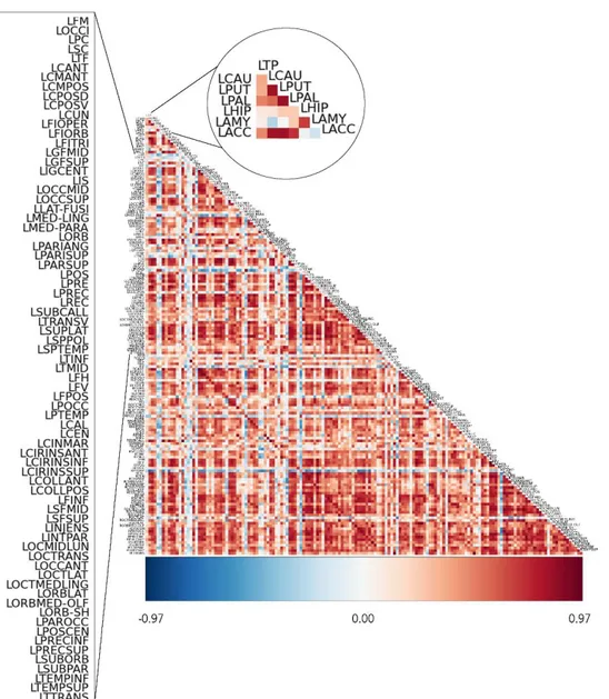
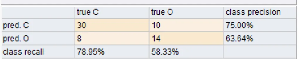
Figure 1 - Graphic representation of a graph. The blue circles are the nodes and the lines are the edges that connect the nodes, making a network. [Adapted from (Boyd, n.d.)] ... 6 Figure 2 - Representation of the organism’s response to an activated brain region. As one can see in the second picture, when an area is activated, the blood vessel is dilated, increasing the blood flow in that specific area. [Adapted from (Devlin, 2007)] ... 13 Figure 3 – Schematic representation of the BOLD hemodynamic response function (HRF). The first vertical dashed line is the stimulus beginning. The response initially takes the form a dip that is only seen at high magnetic field strengths. Afterwards, the response hits a peak, about 4 to 8 seconds after the stimulus and then a negative overshot that dips below the baseline. [Adapted from (Kornak, Hall, & Haggard, 2011)] ... 14 Figure 4 – (A) Block design: stimulus of the same condition are presented subsequently; (B) event-related design: each stimulus’ hemodynamic response is detected, and can be analyzed in detail; (C) mixed design: combination of block and event-related. [Adapted from (Amaro & Barker, 2006)] ... 15 Figure 5 –The Default Mode Network includes areas in the medial pre-frontal cortex, precuneus, and bilateral parietal cortex. [Adapted from (Graner, Oakes, French, & Riedy, 2013)] ... 17 Figure 6 - Resting-state networks. Adapted from (M. P. van den Heuvel & Hulshoff Pol, 2010). 18 Figure 7 - Methods developed for functional connectivity MRI study. [Adapted from (Li et al., 2009)] ... 19 Figure 8 - Representation of a linear classifier that separates objects from two different classes, red and green. ... 27 Figure 9 – Example of a correlation matrix acquired via Nitime Python package. The scale ranges from blue to dark-red, being blue a strong negative correlation and dark-red a strong positive correlation. As one can see in the zoomed-in circle, the LPUT area is less correlated to LPT than it is to LCAU. ... 46 Figure 10 – Example of the results outcome by RapidMiner software. ... 52

xiii

Acronyms List

AUC Area under curve

BOLD Blood Oxygen Level Dependent

CBF Cerebral Blood Flow

CNA Complex Network Analysis

CSF Cerebrospinal Fluid

CT Computerized Tomography

DICOM Default Imaging and Communications on Medicine DMN Default Mode Network

EEG Electroencephalography

EPI Echo-planar Imaging

FA Flip Angle

FC Functional Connectivity

FOV Field of View

fMRI Functional Magnetic Resonance Imaging

FSL FMRIB Software Library

GLM General Linear Model

GM Grey Matter

GNB Gaussian Naive Bayes

GRF Gaussian Random Field

GUI Graphical User Interface

ICA Independent Components Analysis

IT Information Technology

kNN k-Nearest Neighbor

LDA Linear Discriminant Analysis

LR Logistic Regression

MCI Mild Cognitive Impairment

MEG Magnetoencephalography

MI Medical Informatics

MKL Multiple Kernel Learning

MNI Montreal Neurologic Institute

MRI Magnetic Resonance Imaging

NIfTI Neuroimaging Informatics Technology Initiative

xiv

PCA Principal Components Analysis

PET Positron Emission Tomography

RBF Radial Basis Function

RFE Recursive Feature Elimination

ROC Region of Convergence

ROI Region of Interest

RSNs Resting-State Network

SPM Statistical Parametric Mapping

SVM Support Vector Machine

TE Echo Time

TCP Transductive Conformal Predictor

TR Repetition Time

1

1 Introduction

Medical Informatics (MI), as a discipline, is considered young and multidisciplinary. The first use of Information Technology (IT) dates back to the 50’s and since then it has been rapidly expanding and evolving. Thus, it establishes one of the grounds of medicine and health care and, consequently, is responsible for improving the health of people. MI contributes to a better and more efficient health care as well as encourages groundbreaking research in biomedicine and health-related computer sciences (Haux, 2010). Given its multidisciplinary character, MI is hard to define, nonetheless it follows a possible definition:

Definition | Medical informatics is the science that underlies the academic investigation and practical application of computing and communications technology to healthcare, health education and biomedical research. This broad area of inquiry incorporates the design and optimization of information systems that support clinical practice, public health and research; modeling, organizing, standardizing, processing, analyzing, communicating and searching health and biomedical research data; understanding and optimizing the way in which biomedical data and information systems are used for decision-making; and using communications and computing technology to better educate healthcare providers, researchers and consumers. Tools and techniques developed from health informatics research have become and will remain integral components of the best strategies in biomedical research and the best practices in healthcare delivery and public health management (University of Virginia, n.d.).

Nowadays, MI is part of a hospital’s daily life, either in recording and storing patient information on hospital database, monitoring patients’ vital signals or in medical imaging diagnosis. Given the fact that this discipline is multidisciplinary, MI can have a role in different areas such as Medical Imaging, Intelligent Systems, Electronic Health Record and Clinical Decision Support Systems. Besides that, this discipline also shows its worth in information processing in order to extract useful knowledge from the massive amount of information that today’s technology produces. Picturing medicine without technology allows us to realize how valuable this discipline is (Haux, 2010).

2

In Portugal, the Associação Portuguesa de Informática Médica was established in the city of Coimbra in November 5th, 1979. This association was created with the intent to promote the use

of Informatics in the public health, medical practice and medical investigation domains, as well as the propagation of this discipline (APIM, 2012). Despite their efforts and the increasing number of work and investigation done at academic level, in practice, this discipline still has a lot of space to grow. Portuguese hospitals have information systems implemented in some departments. An information system is an integrated set of components – hardware, software, infrastructure and people – designed to store, process, and analyze data, as well as report results on a regular basis (Zwass, n.d.). Usually, each department has its own information system. Portuguese health institutions are investing in IT systems, such as information systems, however this investment is not coordinated, resulting in advanced small islands that unfortunately are incapable of communicating with each other (Fonseca, 2011).

Still concerning MI and regarding the present work, there’s an area that stands out – Medical Imaging. This area provides the methods and techniques that allow visual representation of human organs and tissue. Neuroimaging is the subset of Medical Imaging in charge of the application of such procedures to study brain structure and function. These methods and techniques include Computerized Tomography (CT), Positron Emission Tomography (PET), Magnetic Resonance Imaging (MRI), Magnetoencephalography (MEG), and Electroencephalography (EEG).

1.1 Neuroimaging

It has long been an interest of the human being to figure out how the brain works, particularly how it encodes information and interacts with the environment. In order to explore the brain, more and more advanced techniques have arisen for the task, such as functional Magnetic Resonance Imaging (fMRI), EEG and others. EEG is a technique with poor spatial resolution, making it unsuitable for the study of high-level cognitive activities involved with multiple cortices. In its turn, fMRI allows to further explore the brain function as a whole and with a reasonable spatial resolution (Norman, Polyn, Detre, & Haxby, 2006; S. Song, Zhan, Long, Zhang, & Yao, 2011).

3

fMRI is a non-invasive medical imaging technique used to detect neural activation of different brain regions (Ogawa, Lee, Kay, & Tank, 1990). In the mid-90’s, Ogawa discovered that oxygen-poor hemoglobin and oxygen-rich hemoglobin were affected by the magnetic field in different ways. This discovery allowed him to take advantage of this contrast in order to map images of brain activity (Stephanie Watson, 2008), so this technique takes advantage from the fact that a local variation in the oxygen levels happens when a brain region is active. Therefore, fMRI allows us to study patterns of brain activity during the performance of tasks (Josephs, Turner, & Friston, 1997) or at rest (B. Biswal, Yetkin, Haughton, & Hyde, 1995) which in turn can be used to characterize various pathological conditions such as schizophrenia (Cohen, Gruber, & Renshaw, 1996), Alzheimer’s disease (Greicius, Srivastava, Reiss, & Menon, 2004), Parkinson’s disease (Haslinger et al., 2001) and non-pathological ones, like healthy aging (Hesselmann et al., 2001).

The brain is often seen as a network, built with several regions, anatomically apart but functionally connected, that share information continuously between each other. Using fMRI to study the brain has led to a new concept described below:

Definition | Functional Connectivity (FC) is the temporal dependence of neuronal activity patterns of anatomically separated brain regions (M. P. van den Heuvel & Hulshoff Pol, 2010).

When two or more distinct and anatomically apart brain regions show synchronous neuronal activity or react in the same way to a common stimulus or task, it is then possible to claim that there is FC between them. This synchrony is usually measured by dependencies between blood oxygen-level dependent (BOLD) signals obtained for different anatomical regions.

Since the mid-90’s, the study of FC has drew the attention of neuroscientists and computer scientists as it opens a new window to the network that is the human brain (Li, Guo, Nie, Li, & Liu, 2009). Once in possession of a large amount of FC data, it becomes essential and relevant to extract useful information and knowledge from it. Different methods have been adopted since then and they range from brain activity mapping, FC analysis through exploratory techniques such as Independent Component Analysis (Comon, 1992) to network analysis via graph theory applied to FC data (J. Wang, Zuo, & He, 2010). A relatively new approach in this area is the use of machine learning, mainly classification algorithms, using measures extracted from neuroimaging data. Such methodologies can be valuable in relation to the development of diagnostic support

4

tools and possible forecast of the occurrence of several diseases (Castro, Gómez-Verdejo, Martínez-Ramón, Kiehl, & Calhoun, 2013; Dosenbach, Nardos, Cohen, Fair, & Al., 2010; Long et al., 2012; Nouretdinov et al., 2011; Wee et al., 2012). Classification through machine learning allows the extraction of useful knowledge from large amounts of data in a more automatic way, hence speeding up the process and reducing the human error fraction.

1.2 Machine Learning

The fundamental goal of a learner is to generalize from its experience. In this context, generalization is the ability to give good and accurate results on unseen new data, based on the experience acquired along the learning process.

Definition | Machine Learning is a branch of computer science that, allied with statistics, is focused on the development and study of algorithms that can learn from data instead of simply following programmed instructions. Or, as Arthur Samuel said in 1959, machine learning is a field of study that gives computers the ability to learn without being explicitly programmed (Samuel, 1959).

A classifier, given a training set, is able to learn the association between an examples’ set of attributes (or features) and its corresponding label. This way, it’s possible to perceive the classifier as a function that, for a given example, returns a prediction of its corresponding label. There are many classifiers, however, the ones frequently used in fMRI data are the Nearest Neighbor (kNN), Logistic Regression (LR), Support Vector Machine (SVM), Gaussian Naïve Bayes (GNB) and Fisher’s Linear Discriminant Analysis (LDA) (Pereira, Mitchell, & Botvinick, 2009).

In particular, the classifier used in (Long et al., 2012) to tell apart between patients with early Parkinson’s disease and control subjects was obtained from the SVM method applied to structural and functional images of the participants. This classification method was also used in (Wee et al., 2012) to identify patients with Mild Cognitive Impairment (MCI) and in (Dosenbach et al., 2010) to predict the maturity of the brain from fMRI images. Less frequently used methods include the Multiple Kernel Learning (MKL) described in (Castro et al., 2013) to distinguish between individuals with schizophrenia and control subjects and also the Transductive Conformal Predictor

5

(TCP) algorithm that can calculate the degree of confidence of the prediction given and is described in (Nouretdinov et al., 2011).

Machine learning and pattern recognition are becoming more and more frequent between the chosen techniques to perform fMRI analysis. These techniques allow to detect subtle, non-strictly localized effects that may be invisible to conventional analysis with univariate statistics (Haynes & Rees, n.d.; Martino et al., 2008; Norman et al., 2006). This technique enables the investigator to take into account the pattern of activity from the whole brain. This activity, in its turn, is measured in several points at the same time (i.e. simultaneously). This technique also allows exploring the inherent multivariate nature of fMRI data.

Multivariate pattern analysis is the application of machine learning techniques to fMRI data and typically involves four steps: (Martino et al., 2008)

1. The selection of voxels (features);

2. The representation of brain activity as points in a multidimensional space; 3. The training of the classifier, with a subset of examples, to define the decision boundary;

4. The performance evaluation of the model created.

1.3 Graph Theory

Today’s techniques, whether in the Neuroscience context or in other scientific fields, can provide very large datasets. In the Neuroimaging field, these datasets usually contain anatomical and/or functional connections patterns. In the attempt to characterize these datasets, a new approach has been developed over the last 15 years. This multidisciplinary approach is known as Complex Network Analysis (CNA) and has its origin in the mathematical study of networks, known as Graph Theory (Berge & Doig, 1962). However, this analysis deals with real-life networks above all, which are large and complex (not uniformly random nor ordered) (Rubinov & Sporns, 2010). This method describes complex systems’ relevant properties by quantifying topologies of their respective network representations.

6

Definition | Graph Theory is a branch of mathematics that deals with the formal description and analysis of graphs. A graph (see Figure 1) is defined simply as a set of nodes (vertices) linked by connections (edges), and may be directed or undirected. When describing a real-world system, a graph provides an abstract representation of the system’s elements and their interactions (Bullmore & Sporns, 2009).

Figure 1 - Graphic representation of a graph. The blue circles are the nodes and the lines are the edges that connect the nodes, making a network. [Adapted from (Boyd, n.d.)]

In the context of brain networks, the analogy between the brain and a graph is more than useful, it’s intuitive. Since the brain consists of several different areas that are believed to be connected between each other, one good way to depict a brain is by representing it as a complex network, i.e., a graph (Sporns & Zwi, 2004). The areas of the brain can be seen as nodes and the connections between those areas as the edges of the graph.

A graph can be either weighted or unweighted. In the first case, the edges are attributed a value – weight – representing their importance/significance to the network. A more important or prominent connection should have a higher value. In the opposite case, the unweighted graph has no value assigned to each edge. It can be seen as a weighted graph, only every edge has the same value. There are several measures one can obtain in order to characterize a graph and they can be local – referring to a specific node – or global – referring to the network as a whole.

As said, a network is made by nodes and links. In large-scale brain networks, nodes represent brain regions and links can represent anatomical, functional or effective connections. So, in Neuroscience’s context we can find three types of connectivity (Rubinov & Sporns, 2010):

Structural Connectivity: consists of white matter tracts between pairs of brain regions (Greicius, Supekar, Menon, & Dougherty, 2009);

7

Functional Connectivity: consists of temporal correlations of activity between pairs of brain regions, which may be anatomically apart (M. P. van den Heuvel & Hulshoff Pol, 2010);

Effective Connectivity: represents direct or indirect influences that one region causes on another (K. J. Friston, Harrison, & Penny, 2003).

The characterization of structural connectivity and FC as a network is increasing (Bullmore & Sporns, 2009). This is a result of a combination of reasons. The method previously mentioned, CNA, quantifies brain networks in a reliable way and using only a small number of neurobiological meaningful and easy to compute measures (Hagmann et al., 2008; Sporns & Zwi, 2004). The definition of anatomical and functional connections on the same brain map helps to better investigate relationships between structural connectivity and FC (Honey & Sporns, 2009). Also, by comparing structural or functional network topologies between different subject populations it’s possible to detect connectivity abnormalities in neurological and psychiatric disorders (Leistedt et al., 2009; C J Stam, Jones, Nolte, Breakspear, & Scheltens, 2007; Cornelis J Stam & Reijneveld, 2007; L. Wang et al., 2009).

1.4 Problem

Graph theory and machine learning, individually, are not recent fields of investigation, however the combination of both is, especially when applied to FC data. Given the fact that this combination is recent, there isn’t much knowledge available on how to better take advantage of them together. The “know-how” is still very limited.

The use of machine learning in neuroimaging data is already a step ahead of statistical inference, because it allows to identify which features are relevant to distinguish two groups instead of just knowing that a significant difference exists between the groups. The arrangement of these three fields of investigation - machine learning, graph theory and FC - is a complex process that has a lot of potential.

The more knowledge there is about this combination, the easier is to build user-friendly software with graphical and/or command line interfaces, which are more accessible to researchers and allows them to focus on their research questions (Hanke et al., 2009). Besides investigation, these tools can also be relevant for diagnosis purpose, in a way that they might help detecting

8

neurological and psychiatric disorders at an early stage, thus bringing the application of functional neuroimaging to clinical settings.

1.5 Goals

The present work is mainly aimed to explore the use of machine learning algorithms applied to FC data in order to explore their suitability to neuroimaging studies. To this end, a selection of classification algorithms is proposed, as well as the implementation of such selection to the obtained FC data. Furthermore, the FC data will be used to create complex networks. Topological measures of these networks together with the FC data and brain regional volumes will be used as attributes to perform the classification tasks. Finally, a study of the accuracy of these algorithms on the distinction between a group of healthy subjects and subjects with a properly diagnosed neurological pathology, in this case, Obsessive Control Disorder (OCD), will be performed.

One of the issues of FC analysis is the consequential large amount of data. And since data is definitely not the same as knowledge, the need to “dig” for useful knowledge urges. Classification algorithms are somewhat similar to data mining and its use in neuroimaging is increasing, although there isn’t much knowledge on how to implement them. Thus the goal of the present work is to investigate the best way to apply machine learning algorithms to FC data derived from graph theory analysis. There are many classifiers that can be used, and for each one of them, there are several parameters that can be adjusted in order to obtain a better performance. Knowing this, it’s impossible to state that one classifier is better than the rest. There is no absolute truth about this matter, because it depends on the context of the classification problem, the data’s nature and, of course, the combination of the parameters. Hence the purpose of this work is to explore the best combination of parameters and which classifiers to implement in the context of neuroimaging, particularly, FC data.

Other approaches could have been the focus of the present work. Instead of machine learning, for instance, statistic inference could have been used. This approach consists in the process of drawing conclusions about populations or scientific truths from data that is subject to random variation (George Casella & Berger, 2001). Still, since machine learning is somewhat

9

relatively new to the field of neuroscience and appears to be promising in its results, it was, in fact, the path chosen for the present work.

1.6 Structure of the document

This document can be roughly divided in two parts, the first being of introductory and theoretical background while the second comprises the procedures performed throughout the development of this work and the discussion of the obtained results.

Besides the present chapter, chapters 2 and 3 constitute the first part of the document. Chapter 2 introduces the neuroimaging technique that allows the data used, which is fMRI. This technique was discovered by (Ogawa et al., 1990) and is the mother of a relatively new concept that is FC. This technique also allows the investigation of brain activity patterns that can be analyzed through a series of methods, including CNA. This method models the brain as a complex network, where the nodes are brain regions and the edges are connections, functional or anatomical, between the brain areas.

Chapter 3 presents the concept of Machine Learning, which allows to generalize the structure of a certain dataset to unseen data points, given that they are of the same nature as the dataset. In this chapter, the classification algorithms used in the development of the present work are described in detail, as well as some applications of these algorithms to FC data.

Regarding the second part of the document, chapter 4 describes every step and procedure performed throughout the development of this work, starting with the fMRI images and finishing with the attributes and classifiers. This chapter also explains how the correlation matrices were achieved, as well as the complex networks and how the dataset was built.

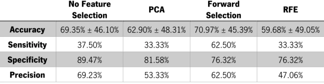
Chapter 5 presents the results obtained for each combination of classifier and feature selection algorithm, as well as the results for each classifier without feature selection. Here, values of accuracy, sensitivity and specificity are presented for each classifier implemented in the development of this work. Comparisons and contextualization with previous results in the neuroimaging field are also presented.

Finally, chapter 6 outlines the conclusions drawn from the results obtained. At this point, is possible to infer which classifier produces the best results, as well as the influence feature

10

selection methods have on the results. Moreover, this chapter presents the main limitations of the work and proposes some improvements that can be made in future works in the field.

11

2 Functional Connectivity

Medical technology has benefited from evolution, so much that it is now possible for imaging scans to create 3D models of organs and tissues of the human body. Moreover, the use of IT in the medical environment has facilitated the recording, analysis and modeling of systems consisting of several interacting elements. These interactions happen in a structured way, resulting in complex and organized patterns that also portray an intrinsic connectivity network. The brain can be seen as one of these systems, constituted by nerve cells that interact with each other and form networks.

Being the brain a target of curiosity and interest as well as an object of study, methods to investigate intrinsic connectivity in this organ have been developed. One of this methods is fMRI, derived from the more conventional MRI, which is a recent technique of imaging that can help diagnose brain diseases, but also investigate human’s mental processes. Both fMRI and MRI are based on the same technology, regarding some differences.

2.1 Magnetic Resonance Imaging

MRI is a noninvasive technique that uses a strong magnetic field and radiofrequency waves to create detailed images of the body. The first time it was used in humans was in July 3, 1977 and it took almost 5 hours to produce one image (Gould & Edmonds, 2010).

This technique takes advantage of the hydrogen atom – abundant in the human body - and its magnetic properties. Initially, the hydrogen atoms are spinning and become aligned when under the influence of a magnetic field. Afterwards, the atoms are hit by a specific radio-frequency pulse, causing them to absorb energy and change their spinning direction, i.e., they are no longer aligned. When the pulse is ceased, the atoms return to the initial alignment, releasing the energy previously absorbed which is picked up by the machine. The signal is then converted into an image by means of the Fourier Transform.

Usually, a superconducting magnet is used. It consists in many coils of wire passed by a current of electricity, thus creating a magnetic field (Gould & Edmonds, 2010). The most common MRI machines yield a 3 Tesla magnetic field, which is equivalent to 50 000x the Earth’s magnetic field. In Tallahassee, vertical widebore magnets are capable of performing MRI with 21.1 Tesla

12

(“National High Magnetic Field Laboratory,” 2014). However, this is not yet used in humans. Stronger magnet fields produce better images but also more noise, making the acquisition much more uncomfortable for the patient, so the typical magnetic field used is of 3 Tesla.

2.2 Functional Magnetic Resonance Imaging

In its turn, fMRI focus on blood flow and detects oxygen levels in the brain, thus providing an indirect measure of neural activity.

Neural activity is an aerobic process, i.e. consumes oxygen 𝑂₂. Given this fact, it’s safe to say that the cerebral metabolic rate of 𝑂₂ consumption and neural activity go side by side, so it’s possible to measure the latter indirectly by means of the former. A healthy brain arterial blood is saturated with oxygen and when this blood arrives to a brain area with increased neural activity and, therefore, with increased 𝑂₂ local consumption, the oxygen gradient across the vessels in that area intensifies. This means that the 𝑂2 molecules are abandoning the hemoglobin, i.e.,

increasing the concentration of deoxyhemoglobin. A higher concentration of deoxyhemoglobin denotes a shorter decay time 𝑇₂∗_{, because it provokes faster de-phasing of excited spins, which, in}

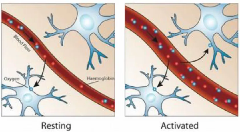
turn, implies a smaller BOLD signal measured at the echo time. However, studies from the beginning of neural activity research with fMRI showed the exact opposite result – the BOLD signal increases with neural activity, hence the deoxyhemoglobin concentration decreases (Ogawa et al., 1992). This divergence can be explained by a phenomenon called neurovascular coupling. Given the 𝑂₂ demand, parallel with increased neural activity, the human body reacts by increasing the cerebral blood flow (CBF), i.e., the vessels dilate locally to enlarge the volume of oxygen-rich blood reaching the area with increased neural activity (see Figure 2). The result of the coupling mechanism overlaps the 𝑂2 consumption, disguising the increase of deoxyhemoglobin

13

Figure 2 - Representation of the organism’s response to an activated brain region. As one can see in the second picture, when an area is activated, the blood vessel is dilated, increasing the

blood flow in that specific area. [Adapted from (Devlin, 2007)]

2.2.1 BOLD

The imaging method most used when dealing with brain function is the BOLD contrast. This method is based on MRI images made sensitive to changes in the state of oxygenation of the hemoglobin. The BOLD signal results from the fact that oxyhemoglobin is diamagnetic and deoxyhemoglobin is paramagnetic. This means that oxyhemoglobin has no unpaired electrons in its outer layer and is not affected by the magnetic field. However, deoxyhemoglobin is affected by the magnetic field because it has at least one unpaired electron (Helmenstine, 2014).

Following, Eq. 1 describes the BOLD signal (Murphy, Birn, & Bandettini, 2013):

𝑆 = 𝑀0exp (−𝑇𝐸_𝑇

2∗) Eq.1 Where:

𝑆 = BOLD signal strength 𝑀0 = Initial magnetization

𝑇𝐸 = Echo time (at which the image is acquired) 𝑇2∗ = Decay time

The initial magnetization (𝑀0) depends on the number of excited spins in a voxel and the

changes in the decay time (𝑇₂∗_{) are the basis for the BOLD signal. 𝑇}

2∗ is the inverse of the relaxation

14

is chosen to maximize the BOLD contrast and, for a 3 Tesla magnetic field, is usually 30 ms (Murphy et al., 2013).

The brain volume consists in several voxels – a volume unit that can be portrayed as a pixel with a third dimension. For each voxel, the BOLD signal is measured over a period of time, resulting in a timeseries for each voxel. In Figure 3, a schematic representation of the BOLD signal is presented.

Figure 3 – Schematic representation of the BOLD hemodynamic response function (HRF). The first vertical dashed line is the stimulus beginning. The response initially takes the form a dip that

is only seen at high magnetic field strengths. Afterwards, the response hits a peak, about 4 to 8 seconds after the stimulus and then a negative overshot that dips below the baseline. [Adapted

from (Kornak, Hall, & Haggard, 2011)]

2.2.2 Task-related fMRI

Task-related fMRI is the most common of fMRI acquisition and is used to detect neural activity in response to a determined event, by means of the BOLD signal. When performing a task-related fMRI, the patient must perform an a task, whether talk, answer questions via response pads, move a finger or simply visualize images (Josephs et al., 1997). There is a wide range of fMRI study designs available for neuroscientists who investigate cognition and other brain processes and different acquisition schemes can be used, such as block design or event-related (Amaro & Barker, 2006).

The strategy of a task-related fMRI experiment is to perform some sort of interference in a system (the brain, in this case) and observe the modulation of the system response. In other words, the experimenter executes an action and observes the reaction. Usually the interference caused or the action made is a cognitive task or a stimulus presented to the subject under study

15

and the reaction is measured by the BOLD signal that shows the hemodynamic response to that specific stimulus. The set of structured, temporal organized and ordered tasks or stimulus is called a paradigm.

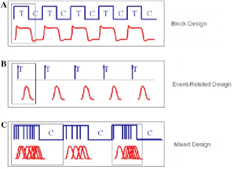
In early days, fMRI studies consisted of stimuli presented in sequence within blocked conditions. The reason for this is the historical influence of PET, because this technique studies had investigated changes in blood flow measured over time periods of up to 1 min, while the subjects had to maintain their cognitive engagement (Amaro & Barker, 2006). Over the years, fMRI has evolved to implement several stimulus presentation schemes, such as block and event-related designs, as well as a combination of both (see Figure 4). Minimum degree of complexity is advised when building a paradigm. Also, the experimenter must formulate a hypothesis, preferably with neuroanatomical background.

Figure 4 – (A) Block design: stimulus of the same condition are presented subsequently; (B) event-related design: each stimulus’ hemodynamic response is detected, and can be analyzed in detail; (C) mixed design: combination of block and event-related. [Adapted from (Amaro & Barker,

2006)]

Regarding block design, this type of paradigm is based on maintaining cognitive engagement in a task by presenting stimuli sequentially within a condition, alternating this with other moments (epochs) when a different condition is presented. When two conditions are used, the design is called an “AB block” and two epochs of each condition form a “cycle”. The BOLD

16

response is composed from individual hemodynamic responses from each stimulus and is generally higher in magnitude.

In its turn, event-related design is based on the observation that changes in hemodynamics are rapid and occur within seconds after a neuronal event. These events can be the result of presentation of a stimulus, delay period and response. In this case, stimuli are not presented in a set sequence; the presentation is randomized and the time between stimuli can vary. This paradigm design has emerged to better exploit fMRI, which has good temporal resolution and is sensitive to transient signal changes of brief neuronal events (Buckner, 1998), allowing the temporal characterization of the hemodynamic response. For each stimulus, the matching response is collected by the fMRI scanner.

As shown in Figure 4, both block and event-related designs can be used together as a mixed design. In this case, a combination of events closely presented, intermixed with control condition, provides the technical needs for event-related analysis as well as cognitive state information.

2.3 Resting-State fMRI and FC

Resting-state fMRI aims to investigate the brain’s functional connections between different regions of the brain when it is “at rest”. In this case the patient is asked to close his/her eyes and try to think about nothing, instead of performing a task in a task-related fMRI. Resting-state fMRI aims to study the spontaneous synchronous neural activity that happens in the human brain when the subject isn’t particularly focused, i.e., not performing a task, not thinking in something specific.

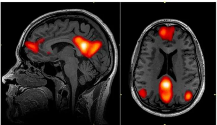
Although the mechanisms behind this neural activity are yet to be known, many resting-state networks have been discovered. The most known is the default mode network (DMN) – see Figure 5. DMN was first discovered using an imaging technique called PET (Raichle et al., 2001), however, fMRI is the preferred tool to further investigate this and other resting-state networks. Its better spatial resolution, compared to EEG and MEG, allows the localization and separation of the various resting-state networks simultaneously (Murphy et al., 2013).

17

Figure 5 –The Default Mode Network includes areas in the medial pre-frontal cortex, precuneus, and bilateral parietal cortex. [Adapted from (Graner, Oakes, French, & Riedy, 2013)]

Compared with task-related fMRI, resting-state fMRI has a downside: since all the voxel’s timeseries are acquired at the same time, the resulting measure of FC can be a spurious result, because one or both timeseries of the brain region in cause could be affected by any non-neural activity at that time. Everything that might affect the FC and is not neural activity related is considered noise and, whenever possible, should be omitted or reduced. This includes the cardiac frequency, as well as the patient breathing movements. This is why the patients are asked to stay as still as possible during the acquisition period.

2.3.1 Functional Connectivity

FC has its foundation in the assumption that temporal similarity between BOLD signals of brain regions denotes that they are connected, thus forming a functional network (M. P. van den Heuvel & Hulshoff Pol, 2010). In order to find these temporal similarities, the BOLD signals from all the brain regions must be correlated against each other to find which areas are active. If two given areas are highly correlated, it means they are active at the same time (or during the same task, in task-related fMRI) and are, presumably, functionally connected.

FC is believed to be vital in complex cognitive processes by allowing a continuous integration of information. Thus, regarding the study and investigation of the human brain structure and organization, the analysis of FC shows to be very important. In neuroimaging, FC depicts the level of communication between anatomically apart brain regions, by describing the neuronal activity patterns of those regions.

18

2.3.2 Resting State Networks

Several resting-state networks (RSNs) have been identified over time. RSNs is the designation of a set of brain regions identified in FC studies as being anatomically apart but functionally connected when the brain is at rest. These sets of brain regions can also be designated as low frequency networks, because these networks mostly consist of low frequency spectrums. These networks can be seen in Figure 6, where a schematic representation of the brain areas active in each RSN is shown. In spite of different test subjects, different methods and even different imaging techniques, the results converge to the same resting-state networks (B. B. Biswal, 2012; J. Damoiseaux, 2006; M. P. van den Heuvel & Hulshoff Pol, 2010).

Figure 6 - Resting-state networks. Adapted from (M. P. van den Heuvel & Hulshoff Pol, 2010).

These networks are alleged to be the reflection of intrinsic demands of energy from brain cells - neurons - which go off together with a common functional purpose (Cole, Smith, & Beckmann, 2010; Saini, 2004). It is possible to reliably detect and to reproduce results of the detected RSNs both at individual and group level across a range of analysis techniques (J. Damoiseaux, 2006; Greicius et al., 2004; J. Wang et al., 2010). Moreover, a determined set of co-activating functional systems is consistently found across subjects (C. F. Beckmann, DeLuca, Devlin, & Smith, 2005; J. Damoiseaux, 2006), stages of cognitive development (Cole et al., 2010; Horsch et al., 2007) and degrees of consciousness (Cole et al., 2010; Greicius et al., 2008). Thus

19

enforcing the assumption of RSNs as core functional networks that support perceptual and cognitive processes in the human brain.

2.4 Methods for the investigation of FC

Several methods to analyze fMRI data are described in literature (Li et al., 2009). In fMRI studies, a method called General Linear Model (GLM) is often used (K. Friston & Holmes, 1995). Concerning FC, other approaches are available and include Principal Component Analysis (PCA) (K. Friston & Frith, 1993), Independent Component Analysis (ICA) (C. F. Beckmann et al., 2005; Calhoun, Adali, Pearlson, & Pekar, 2001), clustering (Cordes, Haughton, & Carew, 2002; M. van den Heuvel, Mandl, & Hulshoff Pol, 2008) and seed methods (Cordes et al., 2002; M. Song et al., 2008). These approaches can be divided in model-dependent methods and model-free (also known as data-driven) methods (M. P. van den Heuvel & Hulshoff Pol, 2010). A flow chart representing an organized view of current methods is visible in Figure 7.

Figure 7 - Methods developed for functional connectivity MRI study. [Adapted from (Li et al., 2009)]

20 STATISTICAL PARAMETRIC MAPPING

This is a model-based method used to find activation patterns consequential from cognitive tasks. Over the years, statistical parametric mapping (SPM) has come to refer to the conjoint use of the GLM and Gaussian Random Field (GRF) theory to make typical inferences about spatially extended data through statistical parametric maps (Li et al., 2009). In few words, SPM uses GLM to estimate the parameters that could explain the data and uses GRF to resolve the multiple comparison problems in making statistically powerful inferences (K. Friston & Holmes, 1995). This method was initially used for FC detection in a resting-state data set by (Greicius, Krasnow, Reiss, & Menon, 2003). All brain voxels go through a scaling and filtering process and are then averaged in a certain seed, which is considered as a covariate on interest in the first-level SPM analysis. Afterwards, the contrast images corresponding to this regressor are determined individually for each subject and enter into a second-level random effect analysis, so to determine the brain areas that show significant FC across all subjects belonging to the dataset. SPM is an extremely univariate approach since a statistic (e.g. t-value) is calculated for every voxel, using the general linear model (Fumiko Hoeft, 2008).

SEED-BASED CORRELATION ANALYSIS

This model-based analysis starts with the a priori selection of a voxel, cluster or atlas region from which the timeseries data is extracted; this is called a seed. This selection can be done based on literature or functional activation maps from a localizer experiment. Afterwards, the data is used as a regressor in a linear correlation analysis or in a GLM analysis so to calculate whole-brain, voxel-wise FC maps of correlation with the seed region. This process is considered univariate because each voxel’s data is regressed against the model apart from the other voxels (Cole et al., 2010; Jo, Saad, Simmons, Milbury, & Cox, 2010). In other words, the correlation between the seed’s timeseries and every other voxels’ timeseries is calculated. The correlation coefficient 𝑟 can be calculated by the Eq. 2.

𝑟 =

21

In the previous expression, 𝑋 is the timeseries from the voxel under the scope and 𝑌 is the timeseries from the seed voxel. In its turn, 𝑋 ̅̅̅̅and 𝑌 ̅̅̅ are averaged timeseries, respectively.

The areas with bigger correlation index are the ones activated at the same time as the seed and are hence functionally connected. This results in a FC map that depicts the functional connections of the predefined brain region (seed) and provides information about which areas are connected to the seed and to what extent. Given that this method is considerably straightforward and simple, some researchers prefer it. However, the information retrieved by the FC map is limited to the seed selected, which makes it more difficult to perform an analysis on the whole-brain scale, because it requires to perform every step for each voxel (M. P. van den Heuvel & Hulshoff Pol, 2010). Another downside concerns the noise that might be present in the seed voxel or region that can influence the timeseries and thus confound the results.

PRINCIPAL COMPONENTS ANALYSIS

This is a technique widely used for data analysis and its fundamental goal is to represent the fMRI timeseries by way of a combination of orthogonal contributors. Each contributor consists in a temporal pattern – a principal component – multiplied with a spatial pattern, called an Eigen map. Next, Eq.3 shows how a timeseries 𝑋 can be represented with principal components.

𝑋 = ∑

𝑆

𝑈

𝑉

In Eq.3, 𝑆𝑖 denotes the singular value of 𝑋, 𝑈𝑖 denotes the ith principal component and

𝑉_𝑖 represents the corresponding eigen map. 𝑃 represents the number of components. Typically, the vectors which contribute less to the data variance are excluded, resulting in refined signal data with most of the signal preserved. The generated eigen maps depicts the connectivity between different brain regions and the bigger the absolute eigen value is, the bigger is the correlation between those brain regions (Li et al., 2009).

This FC technique has been applied to some studies (Baumgartner et al., 2000) but its application has some constrains regarding FC because it fails to identify activations at lower contrast-to-noise ratios when other sources of signal are present, such as physiological noise. In addition, there isn’t a consensus about the optimum number of components. In spite of these disadvantages, this method is good at detecting the extensive regions of correlated voxels. Still, this

22

method can be used as a preprocessing step to achieve dimensionality reduction since it reduces second-order dependency between each component.

COMPLEX NETWORK ANALYSIS

Complex network systems and neuroscience are two study fields that meet to create this new perspective of FC analysis (Bullmore & Sporns, 2009; Onias et al., 2013). In this kind of analysis, commonly, several brain regions are defined as nodes of a network and connections (edges) between regions are modeled as the FC between each pair of regions.

The first step of CNA comprises the selection of the nodes. This can be done by one of three ways, being image voxels, segregation based on brain functional division and anatomical brain divisions. The latter is the most common approach and uses brain atlases to segment the brain in a number of regions that will be the nodes. On the other hand, the links constitute measures of functional or effective connectivity between pairs of nodes. These values have their origin in the timeseries computed from the average hemodynamic response at each node. These timeseries will be correlated against each other for all the nodes, yielding a 𝑁 × 𝑁 symmetric correlation matrix. This matrix can be used to create a network straight way, however it is commonly thresholded in order to obtain a binary matrix or to obtain the 𝑥 percentage of strongest connections (being 𝑥 a value determined by the experimenter). When all matrices are thresholded at the same value for all subjects, it is possible to calculate the desired metrics. Every subject will have a specific value, hence, group averages may be computed and a statistical comparison between different groups can be performed.

This approach has been used by numerous studies that have found complex network changes related to different conditions in basic neuroscience (Schröter et al., 2012), neurology (C J Stam et al., 2007) and psychiatry (Liu et al., 2008).

INDEPENDENT COMPONENT ANALYSIS

Unlike the model-based methods, data-driven methods allow the exploration of whole-brain FC patterns without having to previously define a region of interest or seed. ICA, used in several RSNs studies (C. Beckmann, 2005; Calhoun et al., 2001), is one of these methods.

Starting with a signal that is a combination of several sources mixed together by an unknown process, this method tries to find the unknown signal sources. Particularly, in FC analysis, ICA tries to find a combination of sources that might explain RSNs’ patterns, based on the

23

assumption that the signal sources are statistically independent from non-Gaussian distributions. Iteratively, this method finds the components by maximizing the degree of independence amongst them. ICA analysis can be spatial, when the components are independent in the space domain, or they can be temporal, when the components are independent in the time domain (Sui, Adali, Pearlson, & Calhoun, 2009).

2.5 Other Applications

MRI is not only notable for the flexibility of the image contrast between tissues that it permits but also for the range of anatomical and physiological studies that can be undertaken with this technology. Despite its relative maturity, MRI technology is still very dynamic and new applications are being developed and adopted into clinical practice at an impressive rate.

In cancer patients, MRI is still an essential method to establish the staging of cancer and preferred over CT for specific sites of the body including the uterus and bladder, prostate, ovaries, and head and neck cancer. Contrast-enhanced MRI can reduce the number of biopsies in women with abnormal mammograms; and in difficult cases it can reveal residual cancer and help in treatment planning.

Regarding Magnetic Resonance Angiography (MRA), the increased speed of newer MRI systems, together with improved resolution and software processing methods, allows impressive angiographic imaging results through all of the human body. Given the high quality of MRA images, physicians are able to make clinical decisions based on these images. This way, it’s possible to avoid invasive procedures that would have return the same diagnosis and also to perform a better planning of the treatment procedures.

On the subject of cardiac MRI, recent studies have demonstrated that cardiac magnetic resonance (CMR) can produce images of myocardial perfusion that compare positively with those obtained using positron emission tomography and single photon emission computed tomography (Ibrahim et al., 2002).

As for the central nervous system, the use of perfusion and diffusion imaging is becoming a clinical standard in addition to regular MR imaging to help guide the early treatment of stroke. Furthermore, improvements have been observed in MR spectroscopy for the characterization of brain tumors and the follow-up treatment.

24

Software for the coregistration of fMRI data with images from other radiological modalities continues to be developed. This technology is particularly important for stereo-tactical surgical and radio-surgical treatment planning. (A. Maidment, Seibert, & Flynn, n.d.).

25

3 Machine Learning

Machine learning can be found in a numerous amount of applications, such as spam filtering, optical character recognition, search engines and computer vision (Cortes & Vapnik, 1995; Wernick, Yang, Brankov, Yourganov, & Strother, 2010).

The learning algorithm or classifier must learn a number of parameters called features from a set of examples. After the learning process, the classifier is a model that represents the relationship between the features and the class (or label) for that specific set of examples. Later, the classifier can be used to verify if the features used contain information about the class of an example. This relationship is tested by applying the classifier in another set. The training and testing examples are independently drawn from an “example distribution”; when judging a classifier on a test set, we are obtaining an estimate of its performance on any test set from the same distribution. Quote from (Pereira et al., 2009).

These sets are organized in a matrix where each row is an example and, since an example is a row of features, each column is a feature. The testing set has one column missing – the label. The features can have different weight values (𝑤) amongst them, meaning that some features can be more important than others to the result.

A classifier can be seen as a function that receives an example and returns a class label prediction for that example. The various types of classifiers are distinguished by the specific kind of function they learn (Pereira et al., 2009).

Usually, the data from a classification problem is divided in two sets – the train and test set – and both these sets are constituted by examples. In their turn, these examples are an instance of the problem’s population and each one of them has a group of attributes or features. These features are common for all examples, i.e. all the examples have the same features. However the value of the feature varies amongst the examples. In a simple, yet effective, explanation, please consider the mock data set depicted in Table 1.

26

Table 1 – Mock data set that embodies a typical representation of data concerning classification problems

Car Brand Color Year Condition Car_1 Opel Grey 2010 Good Car_2 Nissan Red 2003 Bad Car_3 BMW Blue 2003 Average

This dataset has 3 examples, identified in the first column. The second, third and fourth columns – Brand, Color, and Year – are the features that characterize the objects. All three objects have the same features, however, not all have the same values. The last column is the attribute that depends from the other three and is considered the target value, i.e., the label. Regarding the test set, the last column is omitted, because that is the value intended to predict by the learner. All 5 columns are considered attributes, however they aren’t all the same. The first and last columns are special attributes because they have a role. The former uniquely identifies each one of the examples and the latter is the target value, i.e., the value that identifies the examples in any way and must be predicted for new examples (Akthat & Hahne, 2012).

The more examples used in the training set, the better the classifier will be. When using voxels in the whole brain, it usually results in a few tens of examples and, at least, a few hundreds of features. A possible outcome of this is a phenomenon called over-fitting, which is the likelihood of finding a function that will produce good results in the training set, however it’s not guaranteed that it will do well in the test set (Pereira et al., 2009). It’s very important to avoid this phenomenon in machine learning because it means the trained classifier, i.e. the obtained model, is not appropriate to use in new data. This happens usually when the number of training examples is low and so the learner may adjust to a specific subset of features that have no causal relation to the target function. Despite the increasing performance in the training examples, the model will deliver bad performance results on unseen (new) data sets.

To avoid this problem, from among the functions with good results, one must chose a simple one. A simple function is one where the prediction depends on a linear combination of the features that can reduce or increase the influence of each one of them. When working with linear classifiers, one can be sure that each feature only affects the prediction with its weight and it doesn’t interact with other features, thus giving us the measure of its influence on that prediction. Learning a linear classifier is equivalent to learning a line that separates points in the two classes

27

as well as possible (Pereira et al., 2009). A representation of a linear classifier is shown in Figure 8.

Figure 8 - Representation of a linear classifier that separates objects from two different classes, red and green.

3.1 Supervised vs. Unsupervised

Usually, machine learning tasks can be divided in two categories - supervised and unsupervised learning.

Concerning supervised learning, the algorithm receives as input a set of data examples as well as their respective output (i.e., label), and the goal is to learn the rule that explains the relationship between the examples and their label. This way, when new examples are supplied to the algorithm, it can predict the label, based on the learned rule.

As for unsupervised learning, the algorithm receives only the data examples and no labels. In this case, trying to find natural groups (or clusters) in the input data is the goal. This can also be used to detect patterns in the input data examples.

3.2 Types of Algorithms

Regarding the classifiers that learn a classification function, these fall into two categories, discriminative or generative models. The first ones’ goal is to learn how to predict straight from the training set of examples. Usually, this requires learning a prediction function with a given parametric form by setting its parameters. In the second case, a statistical model of the join probability, 𝑝(𝑥, 𝑦), of the inputs 𝑥 and the label 𝑦 is learned. This model is capable of generating an example that belongs to a given class. The distribution of feature values on the example is

28

modelled like 𝑝(𝑥|𝑦 = 𝐴) and 𝑝(𝑥|𝑦 = 𝐵), where A and B are two distinct classes. Afterwards, this is inverted via Bayes Rule to classify and the prediction result is the class with the largest probability (Ng & Jordan, 2002).

General consensus shows that discriminative classifiers are almost always preferred over the generative ones. One of the reasons for this is that “one should solve the [classification] problem directly and never solve a more general problem as an intermediate step [such as modeling 𝑝(𝑥|𝑦)]” as Vapnik said (Vapnik, 1998).

3.2.1 Algorithms

Numerous learning algorithms are available nowadays, including neural networks, SVM and as well as simpler ones, such as the kNN, amongst others. Each learning algorithm is unique and requires a specific set of parameters in order to perform. Hence, the performance results may vary with the algorithm used, apart from the dataset used.

From the vast range of learning algorithm existing, some discriminative approaches for machine learning algorithms are described ahead. In these descriptions, the definition of the parameters is included, as well as some theory about each algorithm.

NEAREST NEIGHBOR

kNN is one of the simplest classification algorithms and it doesn’t need to learn a classification function (Pereira et al., 2009), i.e., there is no model to fit. The basis behind this classifier is that close objects are more likely to belong to the same category.

Examples from the test set are classified according to the 𝑘 closest examples - the neighbors - from the training set. Being 𝑛 the number of features, all objects are set in the 𝑛-dimensional space. A new, unlabeled object is also set in the same 𝑛-dimension space and each object in the surroundings adds a vote to one of the possible label classifications. The new object is classified according to the most similar and close objects. This similarity can be measured by the lowest Euclidian distance, for instance. However, there are several ways to measure this distance. When dealing with binary classification problems, i.e. when there are two possible labels to assign, it’s better to choose an odd 𝑘, to avoid tied votes.