Research Article
xTrek: An Influence-Aware Technique for
Dijkstra’s and A
∗
Pathfinders
Gonçalo P. Amador
and Abel J. P. Gomes
Instituto de Telecomunicac¸˜oes and Universidade da Beira Interior, Covilh˜a, Portugal
Correspondence should be addressed to Abel J. P. Gomes; [email protected]
Received 22 October 2017; Revised 23 January 2018; Accepted 7 February 2018; Published 12 April 2018 Academic Editor: Hock S. Seah
Copyright © 2018 Gonc¸alo P. Amador and Abel J. P. Gomes. This is an open access article distributed under the Creative Commons Attribution License, which permits unrestricted use, distribution, and reproduction in any medium, provided the original work is properly cited.
We propose a new pathfinding technique called xTrek that combines conventional pathfinding and influence fields; that is, we are introducing a new influence-sensitive pathfinder or influence-aware pathfinder. The leading idea of influence-aware pathfinding is to avoid unwanted regions and/or converge to desired regions of the search space during the path search. As shown throughout the paper, this region avoidance/convergence is more striking using our technique than in other field-aware pathfinders as, for example, risk-adverse pathfinders and constraint-aware navigation pathfinders. Furthermore, our technique constrains the search space even more than such state-of-the-art influence-aware pathfinders, aiming to reduce the memory space consumption, to speed up pathfinding computations, and at the same time to have better control on the paths to be discovered.
1. Introduction
Artificial intelligence (AI) has many definitions, but Poole et al. [1] describe it as “the study and design of intelligent agents.” An intelligent agent (e.g., NPC, shorthand of on-player character) is an autonomous entity that analyzes the surrounding environment, from where it avoids eventual obstacles, makes decisions, and acts accordingly to achieve its goal or objective [2]. Influence fields, also known as force fields in robotics, are often seen as an obstacle avoidance technique by associating repulsive fields to obstacles. How-ever, influence fields may also work as a trail-orienteering technique by assigning attractive fields to landmarks leading to the desired destination. By combining such repulsive and attractive influence fields, an NPC can follow a collision-free path from a point to another on the game map.
Usually, an NPC is programmed in a loose way to ensure a player has a chance to win a game. NPCs are not intelligent agents in literal terms, but they behave in a seamlessly plau-sible intelligent manner, particularly when they are chasing a player in the game world. For this plausible intelligent behavior, much contributes motion planning algorithms for NPCs and agents [3]. In games, motion planning is known as
pathfinding and has to do with the motion of a given NPC from one place to another in the game world.
1.1. Pathfinders. Before proceeding any further, let us show that pathfinding algorithms are used in many areas other than video games [4, 5], namely, communication network routing [6, 7], robotics path planning [8, 9], and global positioning system navigation systems [10], just to mention a few.
Pathfinding operates over a search graph that describes the path network of the game world. The idea is to find a path (if it exists) between two given locations (two graph nodes), preferably with the lowest cost; in other words, the
pathfinder should be complete and optimal. Dijkstra’s and A∗
[11, 12] pathfinders are two examples of complete pathfinders,
but only the first is optimal; A∗is optimal if the heuristic is
appropriate, that is, if the heuristic function cost estimate is always lower than or equal to the real cost from either node to
the goal of the search. Dijkstra’s is a particular A∗pathfinder
with the heuristic taking on the value 0.
In games, it suffices to use complete pathfinders [13]. Finding the shortest path is not a strict requirement in games, just because such will turn into an advantage for NPCs over Volume 2018, Article ID 5184605, 19 pages
the player. That is, it is harder, not to say impossible, for a player to beat an NPC that acts optimally. Therefore, it is acceptable to propose pathfinding algorithms that sacrifice optimality for performance, as it is the case of the
influence-aware Dijkstra’s and A∗pathfinders introduced in this paper.
These influence-aware pathfinders have the advantage of consuming less memory space, of being faster than their counterparts without influence, and additionally of being context-aware; that is, they avoid unwanted regions and go through preferable regions.
1.2. Influence Fields. In addition to spatial reasoning-based strategy [14–20], influence fields (also known as influence maps) have been also used as an obstacle avoidance technique in motion planning. For example, Ms. PacMan game [21, 22] uses influence fields generated by repulsors and attractors. Repulsors (e.g., ghosts and inedible objects) exert a negative influence, while attractors exert a positive influence (e.g., food, health, or point-scoring objects). That is, repulsors are divergence locations, whereas attractors are convergence locations, regardless of whether they are moving in the game or not. Another example is for activity-centric crowd authoring [23], where influences were used to simulate crowd movement; that is, avatars avoid others yet they converge to areas of interest (e.g., a mall restaurant area).
However, and unlike pathfinders, influence fields were not thought of to find a path between two locations, but at most to induce a steering motion on game entities that move around the environment, yet avoiding obstacles. Recall that an influence field is defined as a function that ascribes a single value (e.g., weight or cost) to each point in game space and time, that is, a concept known in mathematics as a scalar field [24]. It happens that like any other function, an influence field may possess one or more local extrema (i.e., minima and maxima). These local extrema constitute the principal problem of influence fields, because any object moving in the scene may be attracted to and trapped at an extremum. Consequently, influence fields do not ensure that the goal position is reached if one finds a local extremum in the meanwhile.
It is worth noting that a few path planners based on potential fields have been also proposed in the literature [25– 27]. A potential field is also a scalar field, but usually, one takes advantage of a vector field (e.g., the gradient field) associated with it. For example, the path planner introduced by Dapper et al. [26] uses the gradient descent to find routes from any point of the game map to a goal position. The resulting routes are not only smooth but also free of local minima. This path planner was inspired by BVP-based motion planners used in robotics [28], where BVP is the shorthand of boundary value problems. It is not a pathfinder because it uses a motion equation rather than a cost function. However, and similar to grid-based pathfinders, it requires the decomposition of the game map into a grid of square cells. Then, cells spanning obstacles are set to the potential value 1 (repulsors) to avoid collisions, while cells containing target or goal locations for NPCs are set to 0 (attractors). In this BVP framework, each NPC has a local map with a single attractor located at target location so that whenever the NPC moves around in the
environment, its map requires an update to its position and velocity. However, solving the BVP-based motion equation for a given NPC requires the interpolation of the potential values on the grid between obstacle locations and the target location of such NPC [26].
1.3. Related Influence-Aware Pathfinders. At our best knowl-edge, there are five works incorporating awareness of the avatar’s surroundings into pathfinding, yet they differ in their purposes. The first is due to Laue and R¨ofer [29], who used a vector field for navigation of agents in a virtual world. This vector field-based navigation algorithm only takes advantage of a pathfinder when the agent gets trapped at a local extremum. That is, the pathfinder is only used near a local extremum when there is a need to escape from it.
The second work attempts to integrate pathfinders and influence maps and is due to Paanakker [30]. This work
modified the cost functions of Dijkstra’s and A∗pathfinders
to include influence values tied to repulsors and attractors, yet such values are constant within the area of influence of
each repulsor/attractor, that is,−1 for attractors and +1 for
repulsors. This technique is known as risk-adverse pathfind-ing (RAP), so it uses repulsors as risk-adverse entities. It is a repulsor-oriented technique so that a path goes away from repulsors. However, the moving agent often ignores the presence of attractors, walking straight ahead through their influence areas. Furthermore, the behavior of the agent depends on the game map and tuning parameters; that is, the human-like movement behavior that gets out from repulsors and approaches attractors rarely happens and is not automated.
The third work is by Adaixo et al. [31], which replaces such constant influence values by decreasing values obtained from a Gaussian kernel function, but this has not improved the straight moving behavior of agents though attractors (neither repulsors) in a noticeable manner. This problem comes out because there is no guarantee that the cost function value of the next node to be evaluated is less than the cost function value of the current node. In contrast, our field-sensitive pathfinders guarantee that their cost functions monotonically decrease from the start node to the goal node.
The fourth work is due to Sturtevant [32] and incorporates avoidable agents (i.e., agents to avoid) in the process of pathfinding. More specifically, one uses the circular AoI of each agent to be avoided, as well as the distance and the line of sight to it, in the reformulation of the cost-so-far function. Therefore, the AoI plays the role of a repulsor somehow. The idea is to pass by each avoidable agent (e.g., an enemy player) without being seen. However, this technique does not use any concept similar to attractors.
Finally, Kapadia et al. [23, 33, 34] developed influence-aware pathfinders called constraint-influence-aware navigation (CAN) pathfinders. These pathfinders consider both attractors and repulsors, which they called constraints. However, seemingly this technique is not sensitive (or is slightly sensitive at most) to repulsors.
Summing up, among these five techniques, only two integrate influence with pathfinders, namely, risk-adverse pathfinders (RAP) [30] and constraint-aware navigation
(CAN) [23, 33, 34]. However, only the CAN technique is automated; that is, it does not need any manual tuning of parameters. However, CAN only accounts for attractors and repulsors in the proximity of the path found by the traditional
A∗ and Dijkstra’s pathfinders; that is, the convergence to
attractors and divergence from repulsors only occurs if the path found by CAN gets close to the corresponding path by
A∗and Dijkstra’s pathfinders without constraints. In contrast,
the xTrek technique—with “𝑥” standing for either “Dijkstra”
or “A∗”—finds a path that goes toward attractors and deviates
from repulsors. Besides, the placement of attractors and repulsors is also automated and builds upon on the minimum spanning tree of the graph of passable nodes of the game map. In a way, our technique mimics both obstacle avoidance and trail orienteering, whose control points are here repulsors and attractors, respectively.
1.4. Organization of the Paper. The remainder of this paper is organized as follows. Section 2 details the mathemati-cal theory of fields and shows how it can be applied in pathfinding. Section 3 details our influence-aware Dijkstra’s
and A∗ pathfinders, named DjTrek (or DjT) and A∗Trek
(A∗T), including their cost functions that combine the
traditional cost functions with influence functions. Section 4 presents the experimental results obtained from a battery of tests performed for 20 game maps taken from the HOG2 map repository (http://movingai.com/benchmarks/). Section 5 further discusses the applicability of our influence-aware technique in solving the problems of path adap-tivity and smoothness. Finally, Section 6 draws relevant conclusions and points out new directions for future work.
2. Theory of Fields for Games
As explained further ahead, we use attractors and repulsors to guide the agent (avatar) on its way to the goal, avoiding obstacles at the same time. An attractor is a local minimum of a scalar field, while a repulsor is a local maximum of a scalar field. In mathematics, a scalar field ties a scalar value to
every point in space (e.g., 3D Euclidean space orR3). Recall
that a scalar field is known as influence field or influence map
in games. Even considering that the game world𝐷 ⊂ R3 is
bounded in size, the number of points of𝐷 is uncountable, so
we need to discretize𝐷 into a finite number of cubes so that
we then calculate the value of the scalar field at each corner of every single cube. For the sake of convenience, we consider
that𝐷 represents the terrain of the game world; that is, it is
tiled into squares, not into cubes.
A scalar field in R2 is generated by a real bivariate
function𝑓 : R2→ R; that is, 𝑓 is defined at every single point
ofR2. We use a Gaussian function𝑓𝑖to model the scalar field
generated by each repulsor𝑖, which is given by
𝑓𝑖(p) = 𝑎𝑒−𝑑
2
𝑖⋅𝛿2𝑖, (1)
where𝑎 stands for the amplitude of the Gaussian, 𝑑𝑖 is the
distance of an arbitrary pointp ∈ R2to the locationp𝑖of
the repulsor𝑖, and 𝛿𝑖is the decay factor of the Gaussian with
the distance in relation to the location of the repulsor𝑖. More
specifically, we have 𝑎 = 1 2𝜋𝜎2, 𝑑𝑖= p − p𝑖, 𝛿𝑖= 1 √2𝜎, (2)
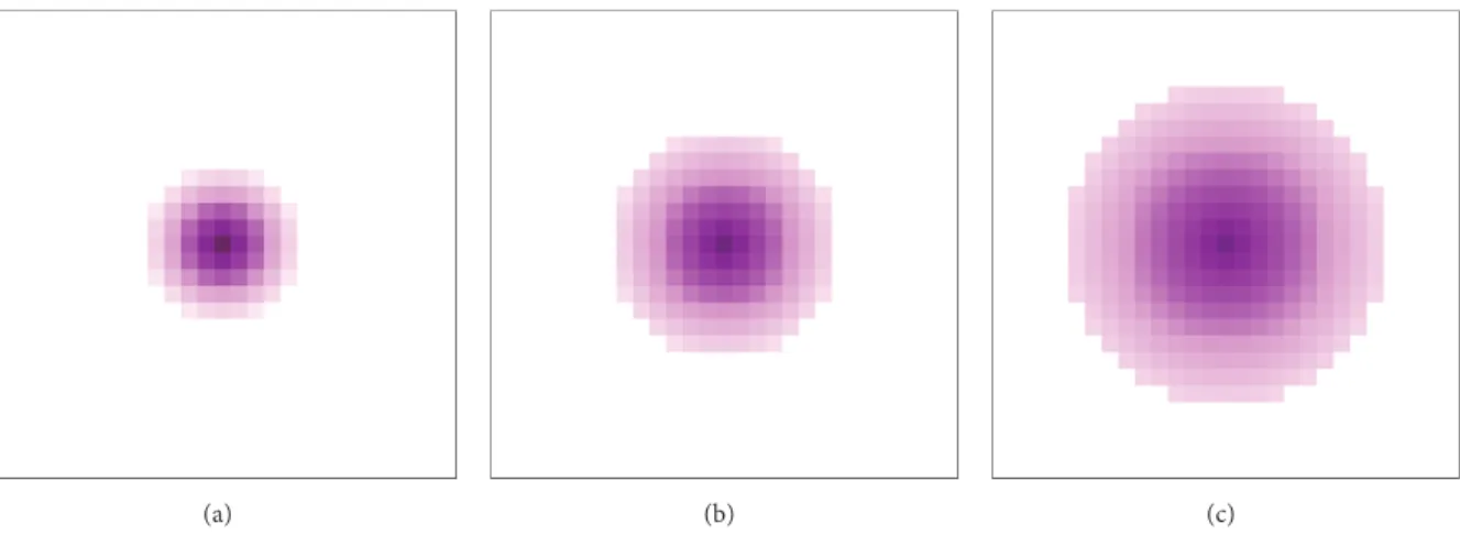
where𝜎 denotes the standard deviation. Figure 1 shows us the
effect of the decay𝛿𝑖on the influence area of a repulsor, so that
the bigger the decay, the lesser the influence area of a repulsor.
Note that each function𝑓𝑖represents the decaying behavior
of the scalar field of the repulsor𝑖 with the distance. That is,
the repulsor is stronger at its location than at any other point in the game world.
On the contrary, an attractor is defined by the negative of Gaussian given in (1) as follows:
𝑔𝑗(p) = −𝑎𝑒−𝑑2𝑗⋅𝛿2𝑗. (3)
Summing up the scalar fields of all repulsors and attractors
results in a scalar field𝐹 of the game world as follows:
𝐹 (p) =𝑛−1∑
𝑖=0
𝑓𝑖(p) +𝑚−1∑
𝑗=0
𝑔𝑗(p) , (4)
where 𝑛 and 𝑚 stand for the numbers of repulsors and
attractors, respectively. In Figure 2, we have 11 attractors in red and 66 repulsors in lilac. Note that repulsors seem less in number because they are side-by-side in adjacent cells.
The main problem with any Gaussian repulsor𝑓𝑖(resp.,
attractor 𝑔𝑗) is that its kernel is unbounded: that is, it
contributes to the value of 𝐹 in (4) at every point of the
game world. Consequently, when a repulsor (resp., attractor)
moves, the overall scalar field𝐹 must be recalculated for every
corner of the terrain tiles. To overcome this problem, one must use truncated Gaussian repulsors (resp., attractors). For every truncated Gaussian repulsor (resp., attractor), we have
thus to consider a small threshold 𝜏 (e.g., 𝜏 = 0.1) below
which the value of|𝑓𝑖| (resp., |𝑔𝑗|) is always zero. Doing so,
it is straightforward to determine the influence radius of each repulsor from (1) as follows:
𝜏 = 𝑎𝑒−𝑑2𝑖⋅𝛿2𝑖 (5)
and, by manipulating (5), we get the influence radius of the
repulsor𝑖, which is given by
𝑑𝑖= 1
𝛿√ln (𝑎𝜏). (6)
So, given the tile size Δ, we can say that the square
influence neighborhood of each repulsor 𝑖 is a 2⌈𝑑𝑖/Δ⌉ ×
2⌈𝑑𝑖/Δ⌉ neighborhood centered at p𝑖, where ⌈𝑑𝑖/Δ⌉ is
smallest integer not less than 𝑑𝑖/Δ. That is, the values of
(a) (b) (c)
Figure 1: Different values for the decay𝛿 of a repulsor: (a) with 𝜎 = √5; (b) with 𝜎 = √10; and with 𝜎 = √20.
(a) (b) (c)
Figure 2: Representation of a grid-based game world: (a) game map; (b) influence map with attractors (in red-to-yellow) and repulsors (in dark lilac-to-light lilac); and (c) game map together with influence map.
from the time they were calculated through (1), regard-less of whether the repulsor moves in the game world or not.
When a repulsor moves around in the game world, what changes is the influence field of the game, which is a discrete
representation of the overall scalar field𝐹 given by (4). We
say “discrete” because, after partitioning the game terrain into
square tiles,𝐹 is evaluated at the center of each tile. Note that
the changes in the influence field are local because they are confined to tiles under the influence of a given repulsor (resp., attractor).
So, the leading idea of the discrete motion planners described in this paper is to fuse a typical pathfinder with a Gaussian influence field, resulting in a pathfinder that avoids obstacles in its way to the goal, without being trapped by
minima. For that purpose, we incorporate the value of 𝐹
(cf. (4)) into cost function of the pathfinder. For simplicity,
attractors were defined by the parameters𝜎 = −√10 and 𝜏 =
0.1, while repulsors were parameterized through 𝜎 = √10
and𝜏 = 0.1 (see (2) and (5)).
3. Influence-Aware A
∗Pathfinders
Before proceeding any further, let us approach the represen-tations for game maps.
3.1. Representations for Game Maps. We only considered grid-based game maps. Each grid-based map is a quadrangle divided into square tiles, also called cells. Each cell is surrounded by eight cells, except if it is a boundary cell of the map; a corner cell has three neighbor cells, while an edge cell has five neighbor cells. Regarding programming, a game map is encoded as a 2-dimensional array of size 𝑙 × 𝑤, where 𝑙 stands for the number of cells along the
length, while𝑤 is the number of cells along the width of
the map. We use these 2-dimensional arrays to host maps retrieved from the HOG repository; more specifically, we used Dragon Age: Origins (DAO) and Warcraft III (W3) maps.
Cells are either passable or impassable. For example, in games like DAO and W3, such cells are as follows:
(i) White cells are passable cells in indoor and outdoor scenarios.
(ii) Black cells are out-of-bounds cells, so they are impass-able cells.
(iii) Green cells correspond to walls and plants, as well as other decorative elements, in indoor scenarios of DAO; in outdoor scenarios as those of W3, green cells denote forests and other obstacles. Therefore, they are impassable.
(iv) Blue cells correspond to deep water, so they are im-passable cells.
(v) Blue sapphire cells are passable, though with a higher cost because they denote shallow water of lakes, rivers, and oceans.
Furthermore, we adopted the following types of cells that do not exist in the HOG format:
(i) Red-to-yellow cells are passable cells and correspond to the circular AoI of each attractor.
(ii) Dark-to-light-lilac cells are passable cells and corre-spond to the circular AoI of each repulsor.
(iii) Cyan cells are passable cells and correspond to cells visited (or explored) by the space search of a given pathfinder.
(iv) Gray cells are passable cells and correspond to doors between different regions of the game map.
For pathfinding purposes, each passable node includes a list of pointers (or references) to its eight neighboring passable nodes at most. We might use a hash map to store neighbor information of each passable node as such data structure has a constant time complexity. However, in practice, it is slower to have the adjacency lists as data of a hash map than having each of them linked to each passable node. This is so because accessing an adjacency list in a hash map using a hash key takes more time than directly accessing such an adjacency list in a passable node.
3.2. A∗ Pathfinding. A∗ search was introduced by Hart et
al. [12] in 1968. Its cost function𝑓(𝑛) comprises two terms,
the cost-so-far function𝑔(𝑛) and a heuristic function ℎ(𝑛) as
follows:
𝑓 (𝑛) = 𝑔 (𝑛) + ℎ (𝑛) . (7)
The cost-so-far function 𝑔(𝑛) stands for the lowest cost to
travel from the current node𝑛 to the start node in the graph.
The heuristic ℎ(𝑛) represents the likelihood of the current
node converging faster to the goal, which is an estimate of the cost to the goal. For example, a possible heuristic is the Euclidean distance from the current node to the goal node.
In other words,𝑔(𝑛) refers to the cost of the current node to
the start node, whileℎ(𝑛) denotes the estimated cost of the
current node to the goal node. Considering only nonnegative
costs, the use of a heuristic means that A∗is solely optimal if
the heuristic is appropriate; that is, the heuristic value must always be less than or equal to the real cost from the current
node to the goal. Dijkstra’s pathfinder [11] is a particular case
of A∗because the heuristic takes on the value zero (ℎ(𝑛) = 0).
Both Dijkstra’s and A∗ pathfinders use identical data
structures, namely, an open list, a closed list, and a graph. The graph holds the passable nodes of the game map, as well as their adjacent nodes. This graph was implemented
as a hash map⟨𝑛𝑜𝑑𝑒, 𝑛𝑒𝑖𝑔𝑏𝑜𝑟𝑠⟩ so that each passable node
representing a game map cell (𝑖, 𝑗) is surrounded by eight neighboring passable nodes at most. Therefore, accessing the nodes neighboring a given node (𝑖, 𝑗) is performed with
complexityO(1).
The open list was implemented as a priority queue, which holds open nodes ordered by increasing costs. An open node is a node in the open list for which the shortest path (i.e., minimum cost) was not found yet. The closed list was implemented as a hash set, which holds closed nodes. A closed node is a node in the closed list for which the shortest path (i.e., minimum cost) was already found; sometimes, a closed node is also called evaluated node. Accessing a closed node using its key (𝑖, 𝑗) has complexity O(1). This key represents the (𝑖, 𝑗)-cell of the game map, but accessing to closed nodes is only for graphics rendering of the cyan nodes that denote the search expansion of the pathfinder. In fact, cyan nodes are the visited nodes of the search space, which include closed nodes and open nodes, as shown, for example, in Figure 3. Note that closed nodes will never be reopened because we assume that all costs are greater than or equal to zero.
3.3. Influence-Aware A∗Pathfinding. The present paper intro-duces a technique to reduce the resources (i.e., memory space
and processing time) usually ascribed to A∗ pathfinders,
including Dijkstra’s pathfinder. Such reduction is achieved by
combining A∗search with an influence field generated by the
Gaussian function𝐹(𝑛) given by (4) as follows:
𝑓 (𝑛) =𝐹MIN− 𝐹 (𝑛)
𝐹MIN ⋅ 𝑑, 𝐹(𝑛) < −𝜏, (8)
𝑓 (𝑛) = 𝑔 (𝑛) + ℎ (𝑛) , 𝐹 (𝑛) ∈ [−𝜏, 𝜏] , (9)
𝑓 (𝑛) = 𝑔 (𝑛) + 𝐹 (𝑛) ⋅ 𝑁 ⋅ 𝑑, 𝐹 (𝑛) > 𝜏, (10)
where𝑛 is the current node (under evaluation), while 𝑁 is
the total number of nodes;𝐹(𝑛) is the influence value at the
current node as yield by (4); 𝐹MIN is the (negative) global
minimum of the influence map, which corresponds to the
value of the influence at the center of some attractor;𝜏 defines
the influence radius of an attractor/repulsor as given by (5);𝑑
stands for the Euclidean distance between the centers of two
connected neighboring nodes. If𝑑 is the horizontal distance
between two nodes, we only get paths along𝑥- and 𝑦-axes,
but, if𝑑 is the diagonal distance between two nodes, we obtain
paths along diagonals in addition to paths along𝑥- and
𝑦-axes (see Figures 3, 4, and 5). The cost function𝑓(𝑛) given
by (8)–(10) also applies to Dijkstra’s pathfinder by setting ℎ(𝑛) = 0.
For simplicity, we assume𝑓(𝑛) ≥ 0, ∀𝑛 ∈ N; that is,
all costs are positive or zero. This assumption avoids getting
(a) (b) (c) (d)
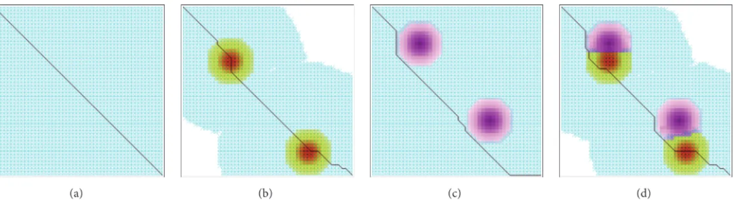
Figure 3: Finding a path (in black) from the top-left node to the bottom-right node of a 50× 50 grid using our influence-aware Dijkstra’s
(DjT) pathfinder: (a) without attractors and repulsors, the search space (neutral nodes in cyan) covers the entire map; (b) with 2 attractors, the search space does not cover the entire map, but it counts on neutral nodes (in cyan) and attractor nodes (in red-to-yellow blended with cyan); (c) with 2 repulsors, the search space covers neutral nodes (in cyan) but not repulsor nodes (in dark lilac-to-light lilac); (d) with 2 attractors and 2 repulsors, the search space partially covers neutral nodes (in cyan) and attractor nodes (in red-to-yellow blended with cyan). Nodes in cyan or blended with cyan represent visited nodes, that is, nodes in the open and closed lists.
(a) (b) (c) (d)
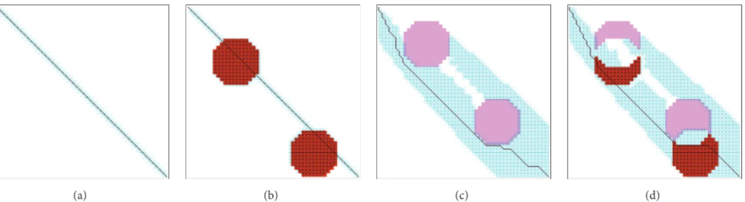
Figure 4: Finding a path (in black) from the top-left node to the bottom-right node of a 50× 50 grid using the risk-adverse Dijkstra’s (DjRAP)
pathfinder: (a) without attractors and repulsors, the search space (neutral nodes in cyan) covers the entire map; (b) with 2 attractors, the search space covers the entire map, including neutral nodes (in cyan) and influence-constant attractor nodes (in red blended with cyan); (c) with 2 repulsors, the search space covers neutral nodes (in cyan) but not influence-constant repulsor nodes (in light lilac); (d) with 2 attractors and 2 repulsors, the search space covers neutral nodes (in cyan) and influence-constant attractor nodes (in red blended with cyan) but not repulsor nodes (in light lilac). Nodes in cyan or blended with cyan represent visited nodes, that is, nodes in the open and closed lists.
(a) (b) (c) (d)
Figure 5: Finding a path (in black) from the top-left node to the bottom-right node of a 50× 50 grid using the constraint-aware navigation
Dijkstra’s (DjCAN) pathfinder: (a) without attractors and repulsors, the search space (neutral nodes in cyan) covers the entire map; (b) with 2 attractors, the search space also covers the entire map, including neutral nodes (in cyan) and attractor nodes (in red-to-yellow blended with cyan); (c) with 2 repulsors, the search space again covers the entire map, including neutral nodes (in cyan) and repulsor nodes (those in purple blue as a result of blending dark-lilac-to-light lilac with cyan); (d) with 2 attractors and 2 repulsors, the search space covers the entire space, including neutral nodes (in cyan), attractor nodes (in red-to-yellow blended with cyan), and repulsor nodes (in purple blue). Nodes in cyan or blended with cyan represent visited nodes, that is, nodes in the open and closed lists.
values, that is, to avoid that the pathfinder gets stuck and stops moving. Equations (8), (9), and (10) produce the values of 𝑓(𝑛) for attractor, neutral, and repulsor nodes, respectively. 3.3.1. Neutral Nodes. These nodes obey (9), which is the cost
function𝑓(𝑛) for A∗and its variants. Neutral nodes are not
subject to the influence of any attractor or repulsor.
3.3.2. Nodes under Influence of an Attractor. Nodes under influence of an attractor obey (8). The AoI of an attractor
includes a central node at which𝐹(𝑛) attains a negative local
minimum𝐹MIN; that is, the value of𝐹(𝑛) decreases from the
attractor’s influence area boundary (i.e., AoI boundary) to its center. This behavior ensures that the path goes through the attractor’s influence area, because the next node of the path is the one with minimum cost in the open list, which is a priority queue sorted by increasing costs, and attractor nodes always have inferior costs compared to neutral and repulsor nodes. In part, this explains why we are not considering the value
of𝑔(𝑛) in (8); otherwise, there would not be any guarantee
to traverse the attractor’s influence area with a noticeable
deflection toward its center. Therefore, discarding𝑔(𝑛) from
(8) allows the path to sense the presence of an attractor; that is, the path deflects toward the attractor center. Note that the
expression|(𝐹MIN− 𝐹(𝑁))/𝐹MIN| varies in the interval [0, 1]
to normalize the values of𝐹(𝑛) in the entire influence field.
3.3.3. Nodes under Influence of a Repulsor. Repelling nodes obey (10). The AoI of each repulsor includes a central node at
which𝐹(𝑛) attains a positive local maximum. In this case, we
can combine𝑔(𝑛) and 𝐹(𝑛) because they are both positive for
a node that is under influence of a repulsor. Intuitively, a node under the influence of a repulsor must have a higher cost than a neutral node or an attractor node. In fact, (10) was designed to endow each node under the influence of a repulsor with less priority (or more costly) relative to any other type of node in the set of open nodes. Therefore, if one does not attain the goal node after searching the entire region of the map outside repulsor’s influence area, the first encountered node under the influence of a repulsor will no longer block path search toward the goal node. In fact, nodes under attractor’s influence will be considered first in the open list, and nodes under repulsor’s influence will be checked later or not at all.
Note that the heuristic is absent in (10) because, when
traveling from the start node to goal node, the cost 𝑔(𝑛)
increases as the heuristicℎ(𝑛) decreases in the traversal of a
repulsor’s influence area. Consequently, the path goes straight across a repulsor’s influence area; that is, the repelling effect is not noticeable. Thus, to mimic the repelling impact on an agent approaching a repulsor, we must guarantee that the global cost is monotonically increasing, hence, the absence
ofℎ(𝑛) in (10).
3.3.4. Behavior of Influence-Aware Dijkstra’s and A∗ Pathfind-ers. The cost function ruled by (8)–(10) is subtle in the sense that it changes the typical behavior of the traditional Dijkstra’s
and A∗ pathfinders. Let us compare the behavior of our
influence-aware Dijkstra’s and A∗ pathfinders (i.e., DjT and
A∗T) with RAP and CAN counterparts.
Regarding DjT pathfinder shown in Figure 3, we observe the following:
(i) Like Dijkstra’s pathfinder, DjT tends to search the entire space.
(ii) However, in the presence of attractors, DjT tends to constrain the space search, as shown in Figures 3(b) and 3(d). This constraint is so because an attractor is a convergence entity that pulls the search to itself. (iii) In the presence of repulsors, the path formed by DjT
goes around each repulsor. Therefore, each repulsor works as a blocker to the path; that is, it fully deflects the path. In fact, as shown in Figures 3(c) and 3(d), the interior nodes of the AoI of each repulsor are not visited at all unless they are also nodes of an attractor. As shown in Figure 4, the risk-adverse Dijkstra’s (DjRAP) pathfinder has a similar behavior to DjT with respect to repulsors because it is adverse to the risk; that is, DjRAP repels above all. However, attractors seemingly do not limit the expansion of the space search. Regarding constraint-aware navigation Dijkstra’s (DjCAN) pathfinder, attractors do not limit the expansion of the search space either, as shown in Figures 5(b) and 5(d). Furthermore, repulsors seemingly do not block paths generated by DjCAN. In fact, as can be observed in Figures 5(c) and 5(d), the interior of the AoI of each repulsor is visited, so the path crosses the AoI of both repulsors.
Regarding A∗T pathfinder shown in Figure 6, we observe
the following:
(i) It also tends to pass through attractors and to avoid repulsors.
(ii) Attractors have even a more striking effect in reducing
the A∗search space than Dijkstra’s pathfinder. Paths
deflect toward attractors when they cross their AoIs (see Figures 6(b) and 6(d)).
(iii) Paths generated by A∗T avoid AoI of repulsors. In
fact, a path does not cross the AoI of a repulsor (i.e., its nodes are not visited), so that each repulsor blocks any path (see Figures 6(c) and 6(d)).
In the case of A∗RAP (Figure 7), its behavior is similar to
A∗T because attractors also constrain search space, while
repulsors expand the search space by blocking the path
being trailed. On the contrary, regarding A∗CAN, attractors
seemingly do not constrain the search space, while repulsors do not entirely block the path being trailed.
4. Experimental Results
Our experimental tests focused on memory space consump-tion and processing time. We compared our field-aware
algorithms, DjT and A∗T, to their counterparts without
influ-ence, Dijkstra’s (point-to-point variant) and A∗ pathfinders,
respectively. We also benchmarked DjT and A∗T relative to
the other four field-aware pathfinders, namely, DjRAP and
4.1. Software/Hardware Setup. We used the Java program-ming language to encode the eight pathfinders mentioned above. Tests were performed on a desktop computer running a Windows 7 64-bit Professional operating system, with an Intel Core i7 2670QM @ 2.2 GHz processor, 8 GB DDR3 RAM, and an NVIDIA GeForce GT 550 M graphics card with 2 GB GDDR3 RAM.
4.2. HOG Dataset. For testing, we used a dataset of 20 game maps taken from the HOG2 [35] map repository (http://movingai.com/benchmarks), 10 of which belong to DAO [36], while the remaining 10 maps concern W3 [37]. Recall that DAO is a role-playing game (RPG), which mostly consists of indoor dungeon-like scenarios. In turn, W3 is a real-time strategy (RTS) game, which is an outdoor game with open scenarios, mostly swamps and islands. The HOG repository does not contain any dataset for first-person shooter (FPS) games.
4.3. Testing Methodology. Before proceeding any further, let us state that we generated an influence map that is congruent with each game map. As shown in Figure 8, nodes within the influence radius of an attractor are depicted in red, orange, and yellow, depending on the distance to the attractor, while nodes within the influence radius of a repulsor are in lilac, with lilacs getting lighter with the distance to repulsor. Note the movement step from a map cell to any of its eight neighbor cells that define four oriented diagonal directions, two oriented horizontal directions, and two oriented vertical directions.
4.3.1. Selection of Paths. In testing, we used four passable nodes to generate 12 paths per map to determine the average memory space expenditure and average processing time. Such nodes are the following: left topmost node A, right top-most node B, left bottomtop-most node C, and right bottomtop-most
node𝐷. Those 12 paths are the following:
(i) Three paths from𝐴 to B, C, and D
(ii) Three paths from𝐵 to A, C, and D
(iii) Three paths from𝐶 to A, B, and D
(iv) Three paths from𝐷 to A, B, and C
Note that the paths from𝐴 to 𝐵 and 𝐵 to 𝐴 can be different
as usual in pathfinding. In fact, even when an optimal pathfinder as, for example, Dijkstra, computes the shortest
path from𝐴 to B, it may create other shortest paths from 𝐴
to𝐵. In testing, we did not allow paths between repulsors,
neither paths between attractors and repulsors (cf. Figures 9 and 10). The reason behind this procedure is because in these cases the search over the graph tends to expand significantly as repulsors have the lowest priority in the process of searching over the graph. Note that the leading idea of influence-aware pathfinders is to constrain the search of the graph representing the map.
Despite the previous testing methodology, nothing pre-vents the placement of an attractor or a repulsor at the starting node, nor at the goal node. However, it does not make sense
to place a repulsor at a goal node, unless we want to delay the arrival of a given NPC to such a node. In fact, when the goal node is assigned a repulsor, the pathfinder first explores the neutral and attractor nodes before evaluating the repulsor nodes in the open list. Recall that the open list works as a priority queue, and repulsor nodes are those with less priority. Thus, a path that ends at a repulsor leads to a more extensive graph search. In the worst case, the search graph may be fully explored before even reaching the repulsor placed at the goal node.
4.3.2. Placement of Attractors and Repulsors. The placement of attractors and repulsors depends on the goals we intend to reach with the game. They may be static or dynamic; for example, a moving enemy may be associated with a repulsor, while an attractor may be a meeting point for some virtual characters. For simplicity, we assume that all attractors and repulsors are static.
The automated placement of attractors in each game map requires the prior generation of its minimal-spanning tree (MST) through Prim’s algorithm [38]. Then, we place attractors along the MST’s minimal path between the start node and goal node of the game map. Alternatively, we might use either a visibility graph [39–41] or a Voronoi diagram [42, 43] to place attractors in the game map. Nevertheless, the MST of each grid-based map has the following benefits:
(i) Similar to the visibility graph and Voronoi diagram, an MST can be precomputed for each map.
(ii) Unlike the visibility graph and Voronoi diagram, the MST of a game map provides some shortest paths between nodes, but many paths are not the shortest ones, as needed to mimic the nonoptimal pathfinding performed by humans when they move around with the necessary space clearance relatively to obstacles. It is worth noting that the visibility graph computes the shortest collision-free path between two nodes (see, e.g., [41, Chapter 15]). However, such shortest paths are tangent to obstacles; that is, there is no space clearance. This lack of space clearance is unnatural, not to say unacceptable, for many motion planning algorithms, including pathfinders. On the contrary, the Voronoi diagram of the obstacles [42– 44] produces paths with maximal space clearance, which may be much longer than the shortest ones. (iii) Also, unlike the visibility graph and Voronoi diagram,
the MST has no cycles, so finding a path between two nodes is straightforward.
Besides, the MST has the advantage of having much less number of nodes and edges to consider in each iteration. In fact, given the hierarchical nature of the MST, it is not necessary to use a common pathfinder (e.g., Dijkstra) to encounter a path between two of its nodes. In a way, the MST works as a global trail-orienteering technique that allows us to place attractors as landmarks along the way between two nodes.
On the other hand, the placement of repulsors in the game map aims at constraining the graph search as much
(a) (b) (c) (d)
Figure 6: Finding a path (in black) from the top-left node to the bottom-right node of a 50× 50 grid using influence-aware A∗algorithm
(A∗T): (a) without attractors and repulsors, the search space only covers neutral nodes (in cyan) along or close to the path (in black); (b)
with 2 attractors, the search space substantially reduces itself to neutral nodes (in cyan) along the path and attractor nodes (in red-to-yellow blended with cyan) provided that they are on the way to the goal node; (c) with 2 repulsors, the search space also substantially reduces itself to neutral nodes (in cyan) along the path, as the interior nodes of repulsors were not visited; (d) with 2 attractors and 2 repulsors, the search space is again limited to neutral nodes (in cyan) and attractor nodes (in red-to-yellow blended with cyan) along the path, with repulsor nodes (in purple blue) not being visited. Nodes in cyan or blended with cyan represent visited nodes, that is, nodes in the open and closed lists.
(a) (b) (c) (d)
Figure 7: Finding a path (in black) from the top-left node to the bottom-right node of a 50× 50 grid using the risk-adverse A∗algorithm
(A∗RAP): (a) without attractors and repulsors, the search space only covers neutral nodes (in cyan) along or close to the path (in black); (b)
with 2 attractors, the search space reduces itself to neutral nodes (in cyan) and influence-constant attractor nodes (in red blended with cyan) found on the way to the goal node; (c) with 2 repulsors, the search space covers neutral nodes (in cyan) found on the way to the goal node, but influence-constant repulsor nodes (in light lilac) repel the search; (d) with 2 attractors and 2 repulsors, the search space covers neutral nodes (in cyan) and influence-constant attractor nodes (in red blended with cyan) but not repulsor nodes (in light lilac). Nodes in cyan or blended with cyan represent visited nodes, that is, open and closed nodes.
(a) (b) (c) (d)
Figure 8: Finding a path (in black) from the top-left node to the bottom-right node of a 50× 50 grid using the constraint-aware navigation
A∗algorithm (A∗CAN): (a) without attractors and repulsors, the search space only covers neutral nodes (in cyan) along or close to the path
(in black); (b) with 2 attractors, the search space almost covers the entire map, including neutral nodes (in cyan) and attractor nodes (in red-to-yellow blended with cyan); (c) with 2 repulsors, the search space covers neutral nodes (in cyan) found on the way to the goal node, and part of the repulsor nodes (those in purple blue as a result of blending light dark-to-light lilac with cyan); (d) with 2 attractors and 2 repulsors, the search space covers the entire map, including neutral nodes (in cyan), attractor nodes (in red-to-yellow blended with cyan), and repulsor nodes (in purple blue as a result of blending light dark-to-light lilac with cyan). Nodes in cyan or blended with cyan represent visited nodes, that is, nodes in the open and closed lists.
(a) (b)
(c) (d)
Figure 9: Distinct paths found within the arena2 map of Dragon Age: Origins by (a) Dijkstra’s, (b) DjT, (c) DjRAP, and (d) DjCAN pathfinders. Cyan nodes are neutral nodes covered by the space search. DjT repulsor nodes in (b) kept their original dark lilac-to-light-lilac colors so that they were not visited. Thus, DjT repulsors contain the space search. However, the same repulsor nodes in (d) appear in purple blue because they were visited, that is, their original dark lilac-to-light-lilac colors were combined with cyan. This color blending occurs because DjCAN does not repel enough: that is, DjCAN repulsors do not sustain the space search. Note that the attractor nodes in (b) and (d) appear in dark red-to-green because they were visited, that is, their original red-to-yellow color was blended with cyan. In (c), we see that repulsors (in light lilac) also sustain the expansion of the search space, but repulsor nodes have the same color because their influence values are constant in DjRAP.
as possible (i.e., to limit the number of visited nodes) to contain the memory consumption and speed up pathfind-ing. Repulsors are just placed at door nodes of the map. Therefore, the automated placement of repulsors in each game map requires the prior computation of its all doors between regions of such map, what is here done using the automated map decomposition algorithm due to Halld´orsson and Bj¨ornsson [45]. As for the MST, the computation of door nodes is performed as a preprocessing step for each game map. For pathfinding purposes, all doors (i.e., door nodes) are closed by default. Closing a door node means to place and turn on a repulsor at its location. Note that we have not turned on all possible repulsors in the figures (e.g., Figures 9 and 10) of this paper for legibility sake. Opening a door node (i.e., turning off its repulsor) only occurs if it is on the
way of the minimum path (of the MST) used to find a path between two nodes (i.e., the start and goal nodes). In other words, closing doors (i.e., turning on repulsors at door nodes) helps the pathfinder to avoid undesirable regions of the map. 4.4. Memory Consumption. Memory consumption has to do with how constrained is the graph search (i.e., the number of evaluated nodes). In fact, memory consumption depends on the number of nodes that have passed by the open priority ordered queue (or simply the open list) and have been moved
into a hash map ⟨ID, 𝑛𝑜𝑑𝑒⟩ of closed nodes. This search
expansion process lasts, while the goal node is not found or the open list gets empty (i.e., no path is found). Thus, the total memory consumption comprises the memory occupied by the nodes that passed on the open list, and this includes
(a) (b)
(c) (d)
Figure 10: Distinct paths found within the arena2 map of Dragon Age: Origins by (a) A∗, (b) A∗T, (c) A∗RAP, and (d) A∗CAN pathfinders.
Cyan nodes are neutral nodes visited during the space search. A∗T repulsor nodes in (b) maintain their original dark lilac-to-light-lilac colors
because they were not visited. Therefore, and like DjT, A∗T repulsors sustain the space search. On the contrary, A∗CAN repulsors in (d) do
not contain the space search because their original dark lilac-to-light-lilac colors were combined with cyan, resulting in purple-blue colored
nodes. This color change means that A∗CAN repulsor nodes were visited. Also, the attractor nodes in (b) and (d) are in dark red-to-green
because they were visited: that is, their original red-to-yellow color was blended with cyan. In turn, the A∗RAP repulsors (in light lilac) in
(c) also sustain the expansion of the space search, though repulsor nodes own the same color because their influence values are constant in DjRAP.
those nodes in the closed hash map. Note that each node 𝑛 comprises the following fields: ID, 𝑔(𝑛), ℎ(𝑛), 𝑓(𝑛), and PID (parent’s ID); PID is required to reconstruct the path backwards.
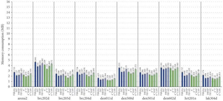
After a brief analysis of the charts shown in Figures 11 and 12, we observe that
(i) W3 consumes more memory space than DAO. This is so because each map’s graph of the former is larger than the largest map of the latter.
(ii) The influence-aware Dijkstra’s pathfinders consume less memory space than Dijkstra pathfinder without influence. Note that DjT ranks first among Dijkstra’s variants for all maps of DAO and W3. For DAO maps, DjT, DjRAP, and DjCAN consume 81.5%,
85.5%, and 94.2% of Dijkstra’ memory space on average, respectively. For W3 maps, DjT, DjRAP, and DjCAN consume 71.7%, 86.3%, and 93.5% of Dijkstra’ memory space on average, respectively. DjT and DjRAP consume the same memory approximately because repulsors constrain the space search, while repulsors seemingly do not constrain the search space of DjCAN.
(iii) In the case of the four benchmarked A∗ pathfinders,
and contrary to A∗CAN, both A∗T and A∗RAP
con-sume less memory space than A∗pathfinder (without
influence). A∗T ranks first among A∗ variants for
all maps of DAO and W3. As far as DAO maps
are concerned, A∗T, A∗RAP, and A∗CAN consume
lak304d hrt201n den602d den501d den500d den011d brc204d brc203d brc202d arena2 0 1 2 3 4 5 6 7 8 9 10 11 12 13 14 15 16 M emo ry co n sum p tio n (MB) 2.735 2.127 2.206 2.495 2.212 1.879 2.024 2.454 4.661 3.81 4.021 4.382 4.109 3.334 2.434 2.048 2.144 2.337 1.997 1.659 1.956 2.286 2.758 2.266 2.437 2.636 2.206 1.926 2.169 2.601 1.633 1.327 1.407 1.564 1.218 1.169 1.292 1.537 3.863 4.31 3.553 2.779 2.87 3 .31 2. 77 2.458 2.639 3.272 2.698 2.284 2.405 2.581 2.245 2.095 2.285 2.557 3.591 3.28 3.425 3.591 3.465 3.045 3.326 3.585 2.727 2.048 2.154 2.529 2.157 1.856 2.021 2.48 2.174 1.606 1.676 1.854 1.575 1.42 1.562 1.813 Di jkstra DjT DjRAP DjCAN T RAP CAN ! ∗ ! ∗ ! ∗ ! ∗ Di jks tra DjT DjRAP DjCAN T RAP CAN ! ∗ ! ∗ ! ∗ ! ∗ Di jkstra DjT DjRAP DjCAN T RAP CAN ! ∗ ! ∗ ! ∗ ! ∗ Di jks tra DjT DjRAP DjCAN T RAP CAN ! ∗ ! ∗ ! ∗ ! ∗ Di jkstra DjT DjRAP DjCAN T RAP CAN ! ∗ ! ∗ ! ∗ ! ∗ Di jks tra DjT DjRAP DjCAN T RAP CAN ! ∗ ! ∗ ! ∗ ! ∗ Di jkstra DjT DjRAP DjCAN T RAP CAN ! ∗ ! ∗ ! ∗ ! ∗ Di jks tra DjT DjRAP DjCAN T RAP CAN ! ∗ ! ∗ ! ∗ ! ∗ Di jkstra DjT DjRAP DjCAN T RAP CAN ! ∗ ! ∗ ! ∗ ! ∗ Di jks tra DjT DjRAP DjCAN T RAP CAN ! ∗ ! ∗ ! ∗ ! ∗
Figure 11: Memory space consumption for 10 maps of Dragon Age: Origins.
15.814 0 1 2 3 4 5 6 7 8 9 10 11 12 13 14 15 16 M emo ry co n sum p tio n (MB) 11.031 7.5 8.329 9.875 7.475 6.85 7.572 9.487 14.62 10.42 12.739 13.926 10.207 9.799 10.245 13.614 14.486 10.58 12.301 13.691 10.134 10.057 10.606 13.312 12.159 8.902 10.533 11.621 8.627 8.31 9.186 11.434 11.028 8.023 9.297 10.102 7.461 7.295 8.096 9.953 15.474 9.577 11.365 13.511 9.8 62 8.825 9.939 13.018 13.807 11.102 13.129 13.27 9.237 10.334 10.745 12.905 16.757 12.368 16.22 10.732 10.247 11.053 15.859 9.184 6.521 8.959 8.916 6.18 5.827 6.25 8.566 8.071 5.758 6.839 7.199 6.11 5.239 6.099 7.015 Tranquilpaths Thecrucible Isleofdread Harvestmoon Gardenofwar Frostsabre Dragonfire Divideandconquer Blastedlands Battleground Di jks tra DjT DjRAP DjCAN T RAP CAN ! ∗ ! ∗ ! ∗ ! ∗ Di jks tra DjT DjRAP DjCAN T RAP CAN ! ∗ ! ∗ ! ∗ ! ∗ Di jks tra DjT DjRAP DjCAN T RAP CAN ! ∗ ! ∗ ! ∗ ! ∗ Di jks tra DjT DjRAP DjCAN T RAP CAN ! ∗ ! ∗ ! ∗ ! ∗ Di jks tra DjT DjRAP DjCAN T RAP CAN ! ∗ ! ∗ ! ∗ ! ∗ Di jks tra DjT DjRAP DjCAN T RAP CAN ! ∗ ! ∗ ! ∗ ! ∗ Di jks tra DjT DjRAP DjCAN T RAP CAN ! ∗ ! ∗ ! ∗ ! ∗ Di jks tra DjT DjRAP DjCAN T RAP CAN ! ∗ ! ∗ ! ∗ ! ∗ Di jks tra DjT DjRAP DjCAN T RAP CAN ! ∗ ! ∗ ! ∗ ! ∗ Di jks tra DjT DjRAP DjCAN T RAP CAN ! ∗ ! ∗ ! ∗ ! ∗
Figure 12: Memory space consumption for 10 maps of Warcraft III.
on average, respectively. Regarding W3 maps, A∗T,
A∗RAP, and A∗CAN consume 96.2%, 104.4%, and
133.8% of A∗memory space on average, respectively.
A∗CAN consumes more memory space than A∗
because repulsors do not limit the search space of
A∗CAN.
xCAN pathfinders tend to consume too much memory space because repulsors seemingly are ignored concerning the process of expanding the search space. That is, though
the path deflects from the center of a repulsor, repulsors do not hamper the expansion of the search space, as illustrated in Figures 9(d) and 10(d). Also, xCAN pathfinders seem to ignore the effect of attractors, unless they are in the proximity of the found path. On the other hand, xRAP pathfinders often ignore attractors, and this explains why they
consume more memory than our DjT and A∗T pathfinders,
as illustrated in Figures 9(c) and 10(c). However, as in DjT and
A∗T pathfinders, repulsors have the effect of hampering the
lak304d hrt201n den602d den501d den500d den011d brc204d brc203d brc202d arena2 0 1 · 10−2 2 · 10−2 3 · 10−2 4 · 10−2 5 · 10−2 6 · 10−2 7 · 10−2 8 · 10−2 9 · 100.1−2 0.11 0.12 0.13 0.14 0.15 0.16 0.17 0.18 0.190.2 0.21 0.22 T o ta l time (s) 1.465 ·10 −2 1.152 ·10 −2 1.567 ·10 −2 9.29 ·10 −3 9.49 ·10 −3 4.78 ·10 −3 7.47 ·10 −3 1.69 ·10 −2 1.812 ·10 −2 2.206 ·10 −2 2.139 ·10 −2 2.082 ·10 −2 1.805 ·10 −2 2.15 ·10 −2 1.35 ·10 −2 1.95 ·10 −2 1.139 ·10 −2 1.127 ·10 −2 1.165 ·10 −2 6.35 ·10 −3 9.3 ·10 −3 9.03 ·10 −3 9.57 ·10 −3 1.409 ·10 −2 1.421 ·10 −2 1.389 ·10 −2 8.43 ·10 −3 9.14 ·10 −3 8.42 ·10 −3 9.1 ·10 −3 1.102 ·10 −2 9.13 ·10 −3 1.056 ·10 −2 3.98 ·10 −3 4.91 ·10 −3 9.87 ·10 −3 3.49 ·10 −3 1.038 ·10 −2 5.22 ·10 −3 7.19 ·10 −3 1.679 ·10 −2 1.599 ·10 −2 9.06 ·10 −3 9.73 ·10 −3 9.53 ·10 −3 1.11 ·10 −2 1.488 ·10 −2 1.647 ·10 −2 1.085 ·10 −2 6.92 ·10 −3 9.07 ·10 −3 6.23 ·10 −3 7.33 ·10 −3 9.38 ·10 −3 1.128 ·10 −2 8.79 ·10 −3 1.613 ·10 −2 1.691 ·10 −2 2.266 ·10 −2 2.05 ·10 −2 1.61 ·10 −2 1.057 ·10 −2 1.761 ·10 −2 1.703 ·10 −2 1.303 ·10 −2 4.78 ·10 −3 6.59 ·10 −3 6.73 ·10 −3 1.162 ·10 −2 1.322 ·10 −2 6.72 ·10 −3 7.56 ·10 −3 2.77 ·10 −3 4.57 ·10 −3 8.83 ·10 −3 4.6 ·10 −3 1.208 ·10 −2 5.42 ·10 −3 5.39 ·10 −3 9.13 ·10 −3 Di jks tra DjT Dj RA P DjCAN CAN ! ∗ RAP ! ∗ T ! ∗ ! ∗ Di jks tra DjT DjRAP DjCAN CAN ! ∗ RAP ! ∗ T ! ∗ ! ∗ Di jkstra DjT Dj RA P DjCAN CAN ! ∗ RAP ! ∗ T ! ∗ ! ∗ Di jks tra DjT DjRAP DjCAN CAN ! ∗ RAP ! ∗ T ! ∗ ! ∗ Di jks tra DjT DjRAP DjCAN CAN ! ∗ RAP ! ∗ T ! ∗ ! ∗ Di jkstra DjT Dj RA P DjCAN CAN ! ∗ RAP ! ∗ T ! ∗ ! ∗ Di jks tra DjT DjRAP DjCAN CAN ! ∗ RAP ! ∗ T ! ∗ ! ∗ Di jkstra DjT Dj RA P DjCAN CAN ! ∗ RAP ! ∗ T ! ∗ ! ∗ Di jkstra DjT Dj RA P DjCAN CAN ! ∗ RAP ! ∗ T ! ∗ ! ∗ Di jks tra DjT DjRAP DjCAN CAN ! ∗ RAP ! ∗ T ! ∗ ! ∗
Figure 13: Time performance for 10 maps of Dragon Age: Origins.
0 1 · 10−2 2 · 10−2 3 · 10−2 4 · 10−2 5 · 10−2 6 · 10−2 7 · 10−2 8 · 10−2 9 · 10−2 0.1 0.11 0.12 0.13 0.14 0.15 0.16 0.17 0.18 0.190.2 0.21 0.22 T o ta l time (s) Tranquilpaths Thecrucible Isleofdread Harvestmoon Gardenofwar Frostsabre Dragonfire Divideandconquer Blastedlands Battleground 0.163 0.155 0.136 0.221 0.255 0.261 0.242 0.206 0.203 0.209 0.192 0.141 0.104 0.151 0.148 0.15 0.129 0.128 0.123 0.271 0.232 0.21 0.195 0.231 0.315 0.225 0.179 0.207 0.259 0.218 0.378 0.286 0.272 0.116 0.143 0.134 0.125 4.464 ·10 −2 6.014 ·10 −2 2.348 ·10 −2 4.206 ·10 −2 7.368 ·10 −2 7.156 ·10 −2 8.235 ·10 −2 4.738 ·10 −2 5.462 ·10 −2 7.179 ·10 −2 5.558 ·10 −2 5.865 ·10 −2 5.159 ·10 −2 8.237 ·10 −2 5.121 ·10 −2 6.507 ·10 −2 8.308 ·10 −2 5.766 ·10 −2 9.079 ·10 −2 7.113 ·10 −2 3.259 ·10 −2 6.328 ·10 −2 6.073 ·10 −2 1.826 ·10 −2 8.003 ·10 −2 5.519 ·10 −2 8.687 ·10 −2 4.522 ·10 −2 2.174 ·10 −2 1.801 ·10 −2 2.825 ·10 −2 7.455 ·10 −2 2.767 ·10 −2 4.778 ·10 −2 5.518 ·10 −2 3.822 ·10 −2 1.342 ·10 −2 4.053 ·10 −2 5.363 ·10 −2 4.469 ·10 −2 6.756 ·10 −2 4.48 ·10 −2 7.16 ·10 −2 Di jks tra DjT DjRAP DjCAN ∗CAN!
RAP ! ∗ T ! ∗ ! ∗ Di jkstra DjT DjRA P DjCAN ∗CAN! RAP ! ∗ T ! ∗ ! ∗ Di jks tra DjT DjRAP DjCAN ∗CAN!
RAP ! ∗ T ! ∗ ! ∗ Di jkstra DjT DjRA P DjCAN ∗CAN! RAP ! ∗ T ! ∗ ! ∗ Di jks tra DjT DjRAP DjCAN ∗CAN!
RAP ! ∗ T ! ∗ ! ∗ Di jkstra DjT DjRA P DjCAN ∗CAN! RAP ! ∗ T ! ∗ ! ∗ Di jks tra DjT DjRAP DjCAN ∗CAN!
RAP ! ∗ T ! ∗ ! ∗ Di jkstra DjT DjRA P DjCAN ∗CAN! RAP ! ∗ T ! ∗ ! ∗ Di jks tra DjT DjRAP DjCAN ∗CAN!
RAP ! ∗ T ! ∗ ! ∗ Di jks tra DjT Dj RA P DjCAN ∗CAN! RAP ! ∗ T ! ∗ ! ∗
Figure 14: Time performance for 10 maps of Warcraft III.
noted during testing that the search-constraint pathfinders (i.e., xTrek and xRAP pathfinders) become more efficient in terms of the memory consumption relative to ground-truth pathfinders. This performance improvement indicates that search contention effects become noticeable.
4.5. Time Performance. The time performance depends on the number of iterations (or, equivalently, closed nodes) carried out by each pathfinder. In fact, each iteration picks up a node from the open queue and turns it into a closed node. A brief analysis of the charts in Figures 13 and 14 allow us to conclude the following:
(i) Traversing W3 maps takes longer than DAO maps because W3 maps are more extensive than DAO maps.
(ii) The influence-aware Dijkstra’s pathfinders are faster than Dijkstra’s pathfinder without influence. DjT and DjRAP have similar time performance and perform better than DjCAN for all maps of DAO and W3 because the repulsors constrain the expansion of the search space. For DAO maps, DjT, DjRAP, and DjCAN take 92.7%, 85.7%, and 114.4% of Dijkstra’ processing time on average to walk the 12 paths per
map mentioned above, respectively. Concerning W3 maps, DjT, DjRAP, and DjCAN take 51.3%, 96.1%, and 102.2% of Dijkstra’ processing time on average, respectively.
(iii) In the case of the four benchmarked A∗
pathfind-ers, only A∗T is faster than A∗ pathfinder (without
influence). A∗T ranks first among A∗ variants for
all maps of DAO and W3. Considering DAO maps,
A∗T, A∗RAP, and A∗CAN spend 84.2%, 102.9%, and
139.3% of A∗ time on average to walk the 12 paths
per map mentioned above, respectively. As far as W3
maps are concerned, A∗T, A∗RAP, and A∗CAN spend
69.6%, 136.3%, and 315.5% of A∗ time on average,
respectively. The poor performance of A∗CAN is
because repulsors do not constrain the search space
of A∗CAN.
Finally, we noted that the time performance of the search-constraint pathfinders (i.e., xTrek and xRAP pathfinders) tends to improve with the increasing length of paths when compared with the time performance of ground-truth pathfinders. This improved time performance is so because the effects of search contention become apparent. In short,
DjT and A∗T perform better than other state-of-the-art
influence-aware pathfinders regarding both memory space and time consumption. Furthermore, their performance improves when the map size increases.
4.6. Path Quality. We carried out a study about the quality of the paths generated by both families of pathfinders, Dijkstra
and A∗. Dijkstra’s family includes Dijkstra’s, DjT, DjRAP,
and DjCAN pathfinders, with Dijkstra as the ground-truth pathfinder, because it generates the shortest paths. In turn,
A∗ family includes A∗, A∗T, A∗RAP, and A∗CAN, and A∗
obviously works as the ground-truth pathfinder for this fam-ily, because it also generates the shortest paths. Furthermore, we also considered two scenarios for the placement of trail-orienteering attractors and the turning off of door repulsors: (i) using the minimal path of the MST for any path between 𝐴 and 𝐵 and (ii) using the shortest path generated by Dijkstra
or A∗.
To measure the quality of a path𝑝 between two nodes
𝐴 and 𝐵, we used the ratio 𝑄 = 𝑛𝑠/𝑛𝑝, where𝑛𝑠represents
the number of nodes of the shortest path from𝐴 to 𝐵 (i.e.,
Dijkstra’s path or A∗ path), and𝑛𝑝is the number of nodes
of𝑝. It is clear that the quality of Dijkstra/A∗ paths is 1, as
shown in Figure 15. A brief glance at Figure 15 also shows us the following:
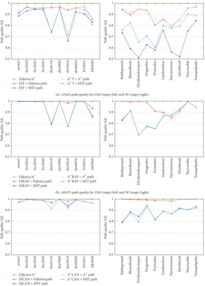
(i) The path quality of xCAN pathfinders (Figure 15(c)) is greater than the one of xRAP pathfinders (Fig-ure 15(b)), which in turn is better than the path quality of xTrek pathfinders (Figure 15(a)), and these facts are valid for W3 and DAO maps. This is so because xTrek and xRAP pathfinders effectively constrain the space search, sometimes forcing NPCs to deviate significantly from the shortest route; for example, such a deviation is remarkable for the DAO map called “den501d.”
(ii) This deviation is more pronounced when one uses
MST’s minimal path, rather than the Dijkstra’s or A∗
shortest path, as the path to follow to place attractors. (iii) As expected, such a deviation relative to the shortest path is not so noticeable when one uses Dijkstra’s or
A∗ shortest path itself as the path to follow to place
attractors.
(iv) The path quality is higher for DAO maps (indoor maps) than for W3 maps (outdoor maps).
(v) In DAO maps (see left-hand side of Figure 15), xTrek
pathfinders (i.e., DjT and A∗T) produce paths of
similar quality when one considers each type of trail-orienteering path separately, either MST path or shortest path. The same applies to both xRAP and xCAN pathfinders.
(vi) In W3 maps (see right-hand side of Figure 15), xTrek
pathfinders (i.e., DjT and A∗T), as well as xRAP (i.e.,
DjRAP and A∗RAP) and xCAN (i.e., DjCAN and
A∗CAN) pathfinders, also produce paths of similar
quality regarding each type of trail-orienteering path separately, and this fact is also true for both xRAP and xCAN pathfinders. The only exception is the xTrek pathfinders when one uses the MST’s minimal paths
as trail-orienteering paths; in this case, A∗T generates
paths of better quality than DjT.
From this comparative analysis based on path quality, we observe the path quality of influence-aware pathfinders is, in general, high or acceptable in the context of games because there is no strict requirement in ensuring the shortest paths. However, when one uses MST’s minimal paths as trail-orienteering paths for the placement of attractors, the path quality is not so high for three out of ten DAO maps, particularly for the maps den011d, den501d, and lak304d. Fur-thermore, the path quality noticeably degrades for W3 maps, especially when one uses MST paths as trail-orienteering paths.
5. Open Issues
The focus of the paper is on how to combine influence fields and pathfinding to obtain more efficient pathfinders regarding memory and time consumption. However, there are open issues like path adaptivity, path smoothness, and multiagent pathfinding whose solutions are in progress.
5.1. Path Adaptivity. Most discrete pathfinders assume that the game map is static; that is, no object moves across the virtual world, no object is being destroyed, and so forth. That is, the search graph remains unchanged. It happens that, in dynamic scenes of game worlds, the graph of passable nodes changes over time indeed; that is, they change their state from passable to impassable, and vice versa. Therefore, we need adaptive pathfinders in games, but as far as we know no adaptive pathfinder has been successful in games,
although they exist in robotics as it is the case of D∗ [46],
ar ena 2 brc 202 d brc 203 d brc 204 d den 011 d den 50 0d den 50 1d den 60 2d hr t201 n lak 30 4d Dijkstra/A∗ DjT + Dijkstra path DjT + MST path A∗T + A∗path A∗T + MST path 0.5 0.6 0.7 0.8 0.9 1 P at h q u ali ty ( Q ) 0.5 0.6 0.7 0.8 0.9 1 P at h q u ali ty ( Q ) Ba tt le gr o u n d Bl aste d lands Di vide an dco nq uer Drag o nfir e Fro st sa b re Ga rdeno fwa r H ar vestmo o n Is leo fdr ea d Thecr ucib le T ra n q u il pa th s
(a) xTrek’s path quality for DAO maps (left) and W3 maps (right)
ar ena 2 brc 202 d brc 203 d brc 204 d den 011 d den 50 0d den 50 1d den 60 2d hr t201 n lak 30 4d Dijkstra/A∗
DjRAP + Dijkstra path DjRAP + MST path 0.5 0.6 0.7 0.8 0.9 1 P at h q u ali ty ( Q ) 0.5 0.6 0.7 0.8 0.9 1 P at h q u ali ty ( Q ) !∗RAP + MST path !∗RAP +!∗path Ba tt le gr o u n d Bl aste d lands Di vide an dco nq uer Drag o nfir e Fro st sa b re Ga rdeno fwa r H ar vestmo o n Is leo fdr ea d Thecr ucib le Tr an q u il p at h s
(b) xRAP’s path quality for DAO maps (left) and W3 maps (right)
ar ena 2 brc 202 d brc 203 d brc 204 d den 011 d den 50 0d den 50 1d den 60 2d hr t201 n lak 30 4d Dijkstra/A∗
DjCAN + Dijkstra path DjCAN + MST path 0.5 0.6 0.7 0.8 0.9 1 P at h q u ali ty ( Q ) 0.5 0.6 0.7 0.8 0.9 1 P at h q u ali ty ( Q ) !!∗CAN + MST path ∗CAN +!∗path Bat tlegr o und Bl aste d la n ds Di vide an dco nq uer Drag o nfir e F rosts ab re Ga rdeno fwa r H ar vestmo o n Is leo fdr ea d The cr ucible T ra n q u il pa th s
(c) xCAN’s path quality for DAO maps (left) and W3 maps (right)
(a) (b) (c)
Figure 16: Close-ups of arena2 map of Dragon Age: Origins for A∗T: (a) without changing the influence field or search graph; (b) after
removing a graph node and its 8 neighbors (in black); and (c) after adding two repulsors at the same location (in blue).
been used in games because it often performs worse than
A∗. This performance drop is so significant that for games
it is preferable to redo the search than using an adaptive pathfinder [47].
On the contrary, DjT and A∗T pathfinders described in
this paper are adaptive; that is, they can deal with game world changes over time, namely, removal/adding a new node and removal/adding of a repulsor or attractor (see Figure 16). More specifically, the following situations require the local reconstruction of a path:
(i) A path includes a bridge that was destroyed by an earthquake. In this case, a subset of passable cells associated with such a road becomes impassable. There is no need to place repulsors in both extremities of the street to get away from such street.
(ii) A path includes a street that was temporarily closed to traffic for some reason. In this case, we need to place repulsors at the entry and exit of the street deal with this situation.
(iii) An obstacle is placed somewhere on a path for some reason. In this case, we need to place at least one repulsor at the location of the obstacle so that the repulsor’s influence goes beyond the area occupied by the obstacle.
(iv) A moving NPC stops on a cell of a path found for another NPC that is approaching it quickly so that such cell becomes the meeting point of both NPCs. The stopped NPC turns on its repulsive shield to force the incoming NPC to deviate from it.
For the local reconstruction of the path, we only need to know where the path interruption starts and ends, applying then the
pathfinder (DjT or A∗T) to a subpath between the new start
and goal nodes. That is, and unlike the usual procedure in other pathfinders, we do not need to reevaluate the nodes of the original path. This is so because we do not need to ensure that each path is the shortest one. In short, path adaptivity is controlled by the placement of repulsors in the game map, though we may use attractors to provoke small deviations to a path. Moreover, the local reconstruction of a path may occur during the backward reconstruction of a path from the goal to the start node or even during the smoothness step.
5.2. Path Smoothness. The discretization of the game map through a grid of cells makes any path looking jagged, even when one uses diagonals (i.e., using an 8-neighborhood to pick up the next node of a path). To endow the human-like movement to an NPC, we must smooth the jagged path, making it a curved path [13]. The typical solution to this problem is using an approximating spline (e.g., a B´ezier spline), but this geometric solution does not guarantee that the path does not collide with obstacles in the scene [48], because of the approximated nature of the curve to the path nodes. To avoid the occurrence of obstacle collisions, we can use an interpolating, rather than approximating, cubic spline [49], but, even so, there is no guarantee of ridding off such collisions, because of the small oscillations of the cubic interpolation spline when it turns right or left. To solve this problem, we combine two tools. The first is the piecewise cubic Hermite interpolating polynomial [50], which does not suffer from shape oscillations. The second is a repulsor placed at each obstacle corner to slightly deviate from the path and get the necessary space clearance for the moving NPC.
5.3. Multiagent Pathfinding. In games, there may be many NPCs moving around a map with the distinct start and goal nodes. In the context of multiagent pathfinding, the
path found using DjT (or A∗T) for each NPC is determined
independently of the existence of other NPCs. That is, an NPC only recognizes its associated trail-orienteering attractors and door repulsors on its way to the goal node; such attractors and repulsors are not sensitive to other NPCs.
To avoid collisions between NPCs, we can associate a repulsor to each NPC, but it is not practical because we would have to recalculate and update the influence field of nodes of each NPC’s AoI whenever it moves around, not to mention the necessary computations whenever another NPC crosses its path. The right way to ensure no collisions between NPCs is to keep their associated repulsors turned off most of the time, and only turning on them where strictly necessary.
Let us imagine two NPCs moving around, A and B, whose
paths meet a point𝑝. If 𝐴 attains the meeting point 𝑝 before
𝐵 without stopping, or vice versa, there no need for action because there is no collision between them, so there is no need to turn on the repulsor of one of them. However, some