A multiple-indicator latent growth mixture model to track courses with low-quality teaching

Repositório ISCTE-IUL

Deposited in Repositório ISCTE-IUL:

Deposited version:

Peer-review status of attached file:

Citation for published item:

Guerra, M., Bassi, F. & Dias, J. G. (2020). A multiple-indicator latent growth mixture model to track courses with low-quality teaching. Social Indicators Research. 147 (2), 361-381

Further information on publisher's website:

Publisher's copyright statement:

This is the peer reviewed version of the following article: Guerra, M., Bassi, F. & Dias, J. G. (2020). A multiple-indicator latent growth mixture model to track courses with low-quality teaching. Social Indicators Research. 147 (2), 361-381, which has been published in final form at

https://dx.doi.org/10.1007/s11205-019-02169-x. This article may be used for non-commercial purposes in accordance with the Publisher's Terms and Conditions for self-archiving.

Use policy

Creative Commons CC BY 4.0

The full-text may be used and/or reproduced, and given to third parties in any format or medium, without prior permission or charge, for personal research or study, educational, or not-for-profit purposes provided that:

• a full bibliographic reference is made to the original source • a link is made to the metadata record in the Repository • the full-text is not changed in any way

The full-text must not be sold in any format or medium without the formal permission of the copyright holders.

Serviços de Informação e Documentação, Instituto Universitário de Lisboa (ISCTE-IUL) Av. das Forças Armadas, Edifício II, 1649-026 Lisboa Portugal

Phone: +(351) 217 903 024 | e-mail: administrador.repositorio@iscte-iul.pt https://repositorio.iscte-iul.pt

1

A multiple-indicator latent growth mixture model to track courses with low-quality teaching

Abstract

This paper describes a multi-indicator latent growth mixture model built on the data collected by a large Italian university to track students’ satisfaction over time. The analysis of the data involves two steps: first, a pre-processing of data selects the items to be part of the synthetic indicator that measures students’ satisfaction; the second step then retrieves heterogeneity that allows the identification of a clustering structure with a group of university courses (outliers) which underperform in terms of students’ satisfaction over time. Regression components of the model identify courses in need of further improvement and that are prone to receiving low classifications from students. Results show that it is possible to identify a large group of didactic activities with a high satisfaction level that stays constant over time; there is also a small group of problematic didactic activities with low satisfaction that decreases over the period under analysis.

Keywords: higher education, quality of didactics, latent growth mixture models, outlier detection, synthetic indicator, data science.

1. Introduction

In recent years, the expansion of the education sector has been the source of much concern and attention, in particular, in relation to the quality of the service provided and the satisfaction of students and other involved publics, seen as consumers (Harvey and Green 1993, Nixon et al. 2016). Students’ participation in university life, as well as their perception and evaluation of teaching quality, play a major role in higher education. In fact, the role of students seems to be a relevant part of the teaching evaluation process, and students’ evaluations of teaching (SETs) have become an almost universally accepted method of gathering information about the quality of education (Zabaleta 2007). The service provided and consumer satisfaction in higher education can benefit from benchmarking other services industries with a long tradition of attention to both the quality of the service provided and customer satisfaction. This could increase loyalty and create stronger ties with alumni and positive word-of-mouth effects. Additionally, student opinion surveys on the university are input for the construction of most rankings in the academic world (see, as an example, The European Teaching Ranking published by Times Higher Education). On the other hand, dissatisfied students may drop out of higher education or move to another institution. Further, this procedure fosters continuous advances in terms of programs, campus facilities, and other attributes. Research on SETs addresses issues such as the importance of involving students in evaluation processes as well as the need to obtain meaningful information that could be used for improvement (Svinicki and McKeachie 2013, Theall and Franklin 2007, Zabaleta 2007). SETs are considered a valuable

2

tool designed to enhance both students’ learning and teaching performance but this is only true if their results are interpreted and used to develop teaching and if students’ feedback is transformed into a stimulus for improvement (Zabaleta 2007). Students’ participation and involvement in the higher education assessment processes is fundamental to promote a growing awareness of their role as stakeholders, as underlined in many European documents (European University Association 2006). Thus, it is important that students’ satisfaction with the service provided is measured regularly to evaluate the different attributes involved and assist in decision making. However, recent literature has also debated the potential drawbacks connected with the use of SETs to assess teaching quality. Uttl et al. (2016), for example, in their meta-analysis found that in many cases there is no significant association between SETs and achievement in subsequent exams on the same subject. According to these authors, the idea that students learn more from highly rated professors is not always verified; indeed, the students’ evaluation is more a measure of satisfaction than of teaching effectiveness. Similar evidence is presented by Boring et al. (2016), while Braga et al. (2014) found a negative correlation between the measure of teacher effectiveness and students’ evaluation. Stroebe (2016) even postulates that when university administration relies on SETs, it induces teachers to adopt didactic practices that students appreciate and not necessarily the ones aimed at improving learning.

Despite this ongoing lively debate (Hornstein 2017), many universities continue to assess the quality of the didactics by means of SETs. In Italy, for example, the Italian Agency for University Evaluation (ANVUR) has made this practice mandatory. This paper seeks to contribute by suggesting a sound procedure to analyze data collected from students about their assessment of teaching in university courses1_{. Although it may not yet be clear if SETs are a measure of}

teaching effectiveness or more an expression of students’ satisfaction, they are in any case an important piece of information that can be processed by university management to monitor and possibly improve the quality of the service. In this strongly competitive environment, higher education institutions need to develop effective decision support tools that accurately inform and assist in all managerial processes (Murias et al. 2008). Developing appropriate academic tools to gather, retrieve, and analyze student data is one of the first steps to be taken (Baker 2014). Data science can play an important role as it extracts patterns using statistical, mathematical and machine learning techniques from large datasets, bringing insights on the meaning of specific patterns that are not easily detected.

Clustering or unsupervised learning is an efficient way to find homogeneous groups in data where members of the same group are more similar to each other than members from different groups. Model-based clustering, also known as finite mixture or latent class models (Lazarsfeld and Henry 1968, Goodman 1974, Clogg 1995, McLachlan and Peel 2000, Wedel and Kamakura 2000, Hagenaars and McCutcheon 2002), has proved to be a powerful paradigm in many

1 _{We use course and didactic activity as synonymous. To be more precise, didactic activity is understood as the}

3

scientific fields as a parametric alternative to heuristic clustering (Dias and Vermunt 2007). This semi-parametric approach assumes that each component of the mixture is a distinct cluster. For instance, Alves and Dias (2015) propose an application to identify clients with different levels of risk in the context of behavioral credit scoring analysis. Indeed, market segmentation has been one of the most important applications of mixture modeling (Wedel and Kamakura 2000). Clustering allows the detection of segments of customers with different levels of perceived service quality and can provide managers with important information about the improvements required. In recent years, the widespread availability of longitudinal data has created the need to identify unique groups or trajectories in populations. This type of data tends to be challenging for any clustering. Heuristic procedures for the classification of time series require the original times series to be transformed into a set of indicators. The first stage in clustering time series data both in statistics and data mining literature was based on adapting the clustering of cross-section data to longitudinal data (Esling and Agon 2012). An alternative approach assumes a latent Markov process in the filtering procedure prior to the heuristic clustering of time series data (Wiggins 1955, Baum et al. 1970, van de Pol and Langeheine 1990, Vermunt et al. 1999, van de Pol and Mannan 2002, Frühwirth-Schnatter 2006, Collins and Lanza 2010, Biemer 2011, Bartolucci et al. 2012, de Angelis and Dias 2014, Dias and Ramos 2014, Zucchini et al. 2016). For instance, a mixture of Markov chains (Dias 2007) and a mixture of hidden Markov models (Dias et al. 2015) have been applied to clustering times series data.

This study does not take the marketing angle as we do not classify customers e.g. into segments. Our focus is on service supply and the detection of critical quality-related situations. Specifically, we proposed a multi-indicator latent growth mixture model (Nagin and Land 1993, Muthén and Shedden 1999, Muthén 2004, Bollen and Curran 2006) with covariates affecting both the latent trajectory and class membership. In addition to the relevant methodologies adopted in the literature to analyze SETs (see, e.g., Rampichini et al. 2004, Bacci et al. 2017, La Rocca et al. 2017), the model proposed herein focuses on the evolution of the quality of the didactics, as judged by the students, over time, allowing heterogeneity among courses and considering also some relevant course characteristic. Given our interest in modeling satisfaction as a latent construct over time, we prefer to rely on the latent growth approach rather than the Markovian approach, which is more suitable to analyze latent dynamics among discrete latent states (Pennoni and Romeo 2017). Hence, we focus on the dynamics of the trajectory as opposed to the dynamics of clustering. Thus, we assume time-invariant clusters of didactic activities with different trajectories of students’ satisfaction.

This model allows university managers to track the progress of courses, identify problematic trajectories of specific courses and act to prevent further damage to course quality and student satisfaction. That is, the framework identifies the universities’ didactic activities that suffer from low-quality teaching. It is illustrated with students’ evaluations of a

4

sample of didactic activities over three academic years from 2012 to 2014 in a large Italian university. The paper is organized as follows: Section 2 describes the case study problem and the data set. Section 3 introduces the latent growth approach. Section 4 presents the results obtained from the model estimation. Section 5 discusses the managerial implications of the results. The final section concludes.

2. The data set

The University of Padua has been collecting information on students’ satisfaction for 15 years. The students’ evaluations of teaching are assigned a major role in the quality assurance system. Since the early 2000s, much attention and extensive resources have gone to gathering high-quality data for the continuous improvement of teaching-learning activities. The survey of students’ opinions supports the various levels of the internal evaluation process; detailed survey results are given to individual professors and managers of the various organizational structures (Course Councils, Departments, Athenaeum Schools). Furthermore, summary results are published on the university website. Specifically, the following indicators are published for each teacher and course: the overall level of satisfaction; an indicator related to the organizational aspects of the course (clarity of scope, examination arrangements, observance of timetable and didactic material); and an indicator related to efficacy of didactics (interest stimulation, clear explanation). A description of the organization of the didactics at the university level in Italy is provided in a recent paper (Meggiolaro et al. 2017).

In the academic years 2012-2013, 2013-2014, and 2014-2015, the questionnaire for the students began with two introductory questions: the first asked if the student was available to participate in the survey, the second asked for the percentage of lessons of the course under assessment that the student had attended. If the student had attended less than 30% of the lessons, he/she was asked to answer only a number of selected questions on some selected items and specifically on why he/she had attended so few classes; otherwise, they were asked to answer all questions.

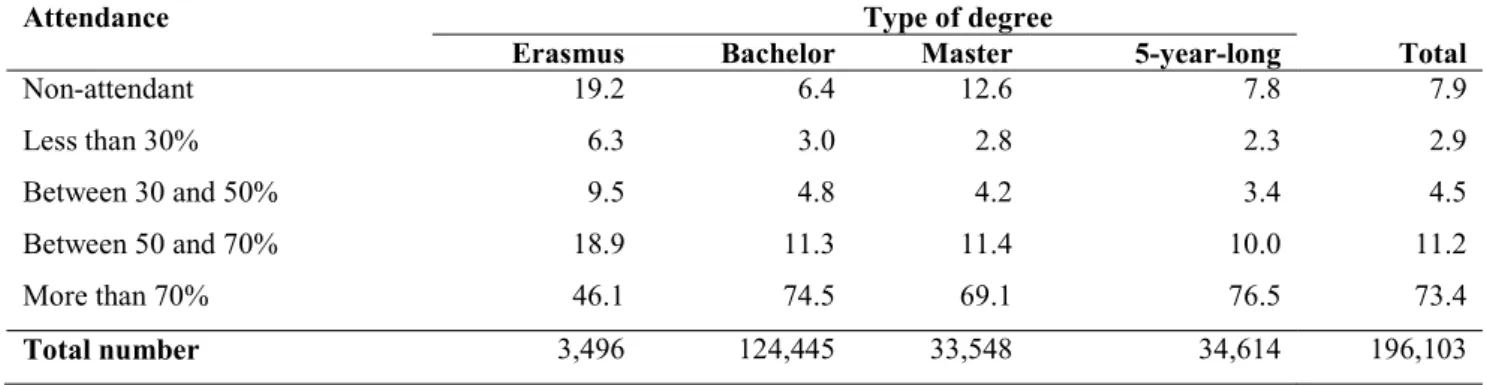
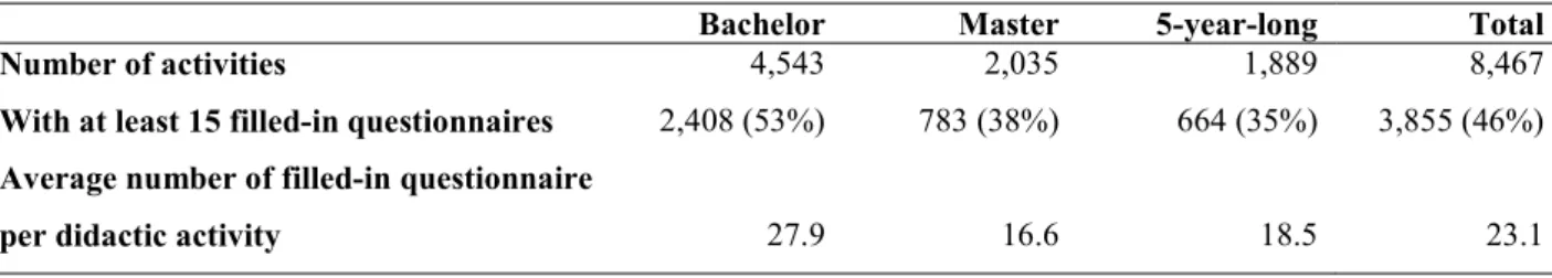
In the academic year 2012-2013, 253,318 questionnaires were administered to the students. Only 196,103 (77.4% of total) were effectively filled in and 57,215 students did not want to participate in the survey with reference to the course they had just attended. Table 1 reports the completed questionnaires classified by the percentage of classes attended by the respondent student and the type of degree in which he/she is enrolled based on the answer to the introductory question. Table 2 lists the number of didactic activities evaluated in the academic year 2012-2013, the number of questionnaires with at least 15 completed forms and the average number of filled-in questionnaires for the degree of the respondent student. Tables 1 and 2 give an idea of the extent of the teaching activity at the University of Padua.

5

==== Table 1 about here ==== ==== Table 2 about here ====

A smaller representative sample was available for our analysis: 1,854 courses (didactic activities) in which there had been no change in teacher or number of teaching hours in the three academic years of reference. Observations with missing data or evident errors were excluded from the analysis, for a total of 11 records (0.6% of the total). Hence, we considered a sample of 1,843 courses taught at the University of Padua in the three academic years. Only questionnaires completed by regular students (i.e. not Erasmus students or enrolled in single courses) who attended at least 50% of the lessons were taken into account. For each course, we also have information on the type of degree (Bachelor, Master or 5-year-long), if it is an elective course attached to a different degree to that of the enrolled student, number of teaching hours and corresponding credits (ECTS), university school where the course is taught, and position of the teacher (assistant, associate, full professor, or other). For reasons of data privacy, all information was anonymized: courses, schools, and teachers were given a code to replace their name. Table 3 contains descriptive statistics with reference to our data set of assessed didactic activities.

==== Table 3 about here ====

The questionnaire contains distinct items covering several dimensions of students’ satisfaction with the courses attended. These items are not exactly the same in the three academic years due to slight changes to the instrument to improve data reliability. Our data set contains only 12 items that remained unchanged during the time frame of academic years under analysis: 11 items concerning specific aspects of the didactic activity, and a general item, the “gold standard”, measuring overall satisfaction. Students were asked to express their level of satisfaction on a scale from 1 (low) to 10 (high). The wording of the 12 items is as follows:

 Item 1 – Were the aims and topics clearly outlined at the start of the course?  Item 2 – Were examination arrangements clearly stated?

 Item 3 – Was the class schedule observed?

 Item 4 – Is preliminary knowledge sufficient to understand all topics?

 Item 5 – Regardless of how the course was taught, how interested are you in the topic?  Item 6 – Does the teacher stimulate interest in the topic?

6

 Item 7 – Does the teacher explain clearly?  Item 8 – Is the suggested study material adequate?  Item 9 – Was the teacher available during office hours?

 Item 10 – If included, are laboratories/practical activities/workshops adequate?

 Item 11 – Is the requested workload proportionate to the number of credits assigned to the course?  Item 12 – How satisfied are you with this course?

We do not have the student level data but only aggregated data that is the arithmetic mean of the sample of respondents in each didactic activity for each year in the study. Nevertheless, a 10-point scale can be reliably treated as interval scales and it allows the computation of arithmetic means (Weng 2004, Wu and Leung 2017).

==== Table 4 about here ====

Table 4 lists the means and the standard deviations for the 12 items, the mean level of satisfaction for the 11 items. Students give lower scores to items 4 (preliminary knowledge) and 11 (workload), higher scores to items 3 (course timetable) and 9 (teacher availability). However, the distribution of judgments is very asymmetric with lower scores used only rarely. Comparing means over time reveals a quite stable situation; only a slight decrease in satisfaction is detected for almost all items. However, these are average values, for almost 2,000 evaluated activities, with non-negligible standard deviations.

3. The model

3.1. The factor-analytic component

Let 𝑦 be the indicator 𝑗, j=1,…,J, for didactic activity i at time t. The responses to the items in the questionnaire from the same didactic activity at a point in time define the latent factor 𝜂 . It is assumed that intercepts and factor loadings are invariant over time. Thus, the factor-analytic component is given by

7

where 𝑦 is the arithmetic mean over the sample of respondents of item j in the questionnaire to evaluate didactic activity i in academic year t, 𝜈 is the time invariant intercept for indicator 𝑗, 𝜆 denotes the time invariant factor loading for indicator 𝑗, and 𝜐 are uncorrelated error terms with variance 𝜎 = 𝑉𝑎𝑟(𝜐 ).

3.2. The latent growth component

The latent growth component links the three waves of the data set to take longitudinal dynamics into account (McArdle and Epstein 1987, Meredith and Tisak 1990, Bollen and Curran 2006). It specifies the latent trajectory of 𝜂 as a result of a random intercept (𝛼 ) and a random slope (𝛽 ):

𝜂 = 𝛼 + 𝛾 𝛽 + 𝝎𝒛 + 𝜖 . (2)

where the usual convention for linear growth2 is that 𝛾 = 𝑡 − 1 and the residuals are normally distributed with variance 𝜃 , i.e., 𝜖 ~ 𝑁(0, 𝜃 ). Time-varying covariates (𝒛 ) are allowed to explain the latent factor. Finally, the random intercept and slope define the trajectory of each didactic activity taking the average trajectory into account.

Conditional latent growth models not only describe the trajectory but also examine predictors of individual change over time. The random effects are, consequently, specified as

𝛼 = 𝜇 + 𝝁 𝒙 + 𝜁 (3)

and

𝛽 = 𝜇 + 𝝁 𝒙 + 𝜁 . (4)

where 𝒙 is a vector containing the value of time-invariant explanatory variables for didactic activity i. The model assumes 𝜁 ~ 𝑁(0, Ψ ), 𝜁 ~ 𝑁(0, Ψ ), and 𝐶𝑜v(𝜁 , 𝜁 ) = Ψ . 𝜁 , 𝜁 , and 𝜖 are mutually independent for every i and t. The parameters of interest are the intercepts, slopes, and variances of the random effects, and the residual variances over time. A second-order growth model is also known as a growth model with multiple indicators since it allows the modeling of the latent trajectory of a variable that is itself not directly observable. This model specification has been used in service quality analysis (see, e.g., Masserini et al. 2017).

3.3. The mixture component

8

The mixture model decomposes the data set into subsets with distinct heterogeneity. Thus, the latent growth mixture model is an extension of the model described in the previous paragraph (Nagin and Land 1993, Muthén and Shedden 1999, Bassi 2016). It relaxes the assumption that considers that all individuals come from the same population and it states that there are different subpopulations characterized by different trajectories (Connel and Frey 2006). The model estimates the intercept and slope for each latent class and didactic activity variation around these growth factors:

𝛼 = 𝜇 + 𝝁 𝒙 + 𝜁 (5)

and

𝛽 = 𝜇 + 𝝁 𝒙 + 𝜁 , (6)

where 𝑘 indicates one of the 𝐾 subpopulations with probability 𝜋 . It is assumed that factor loadings and intercepts of indicators are invariant across clusters and that 𝜁 ~ 𝑁(0, Ψ ), 𝜁 ~ 𝑁(0, Ψ ) and 𝜖 ~ 𝑁(0, 𝜃 ) are independent. Residual variances are kept component-invariant (𝜎 ).

In this specification, each subpopulation, identified by the categories of the latent variable, has its own trajectory over time.

The mixture model can be further extended by allowing covariates to explain the latent categorical variable that defines the mixture. The proportions of the mixture component can be regressed on covariates, called concomitant variables (Dayton and Macready 1988, Formann 1992). Assuming a multinomial logit link function, the probability that didactic activity 𝑖 belongs to component 𝑘, given the set of concomitant variables 𝒘 , is given by

𝜋 = ( 𝜸 𝒘 )

∑ ( 𝜸 𝒘 ), 𝑘 = 1, … , 𝐾 − 1, 𝑖 = 1, … , 𝑛 (7)

where 𝛾 and 𝜸 are the intercept and slopes, respectively. This component of the model is used to estimate the probability of a didactic activity to belong to each component (𝜋 ).

3.4. Conceptual framework

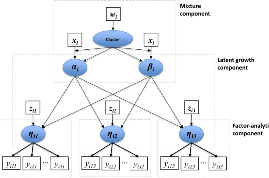
Figure 1 summarizes the model applied in this research. After the selection of the items to be included in the modeling (item pre-selection), a latent growth mixture model that contains the three components previously discussed is specified. Hence, the longitudinal latent factor measuring the time-specific items is assumed to follow a latent growth model conditional to the mixture component. In the case of two components, we expect to detect trajectories that are not doing so well (outliers). Additionally, the trajectory (a component of the mixture) is conditional on characteristics of didactic activities (concomitant variables) that allow easy tracking of the outliers.

9

==== Figure 1 about here ====

3.5. Model estimation and model selection

The maximum likelihood estimation of this latent class model is not available in closed form and the expectation– maximization algorithm (Dempster et al. 1977) is used to obtain the estimates. The decision on the optimal number of mixture components is traditionally given by information criteria (McLachlan and Peel 2000). We report the BIC – Bayesian Information Criterion (Schwarz 1978) and AIC – Akaike Information Criterion (Akaike 1974), whose lower values indicate the most parsimonious model (trade-off between model fit and model complexity). Where there is disagreement between BIC and AIC, we decide on the selection based on BIC due to its good performance in retrieving the right model (Dias 2006). All models are estimated using the statistical software MPlus.

4. Results

4.1. Reliability of the synthetic indicator

Before conducting the modeling, we assess the reliability of the indicators to measure students’ satisfaction. It is of the utmost importance that these indicators, and the instrument by which they are collected, have the properties of validity and reliability that guarantee their purpose. In Dalla Zuanna et al. (2015), the scale has been shown to be reliable and valid following the traditional procedure proposed in the psychometric literature (Churchill 1979) that implies taking a number of steps when developing a measurement instrument. These steps refer to construct and domain definition and scale validity, reliability, dimensionality, and generalizability (Bassi 2010). Factor analysis is a commonly used statistical tool for describing the associations among a set of manifest variables in terms of a smaller number of underlying continuous latent factors (Bartholomew and Knott 1999). Thus, using exploratory factor analysis, a single factor should be identified. Confirmatory analysis checks the goodness-of-fit of the model.

10

The 12 items are highly correlated; all correlation coefficients are greater than 0.67. There is a strong correlation, for example, between items 6 and 7 (0.94), and 7 and 8 (0.91). Scale validity is ensured by the fact that the 11 items are all highly correlated (>0.77) with item 12, which measures overall satisfaction and is considered the “gold standard”. An exploratory factor analysis was conducted of the data set for the three years3_{. Item 12 is excluded as it is already a}

kind of summary measure of the other 11 items assessing didactic activities. Table 5 lists factor loadings, item-to-rest correlation coefficients, and Cronbach’s alpha coefficient when the item is deleted. One factor explains almost 81% of total variance and shows very high standardized loadings, greater than 0.84 for all 11 items. As regards scale reliability, the Cronbach’s alpha coefficient is 0.967, 0.972, and 0.976 for the three academic years, respectively. The values of Cronbach’s alpha when each item is deleted from the scale are all lower than the value of Cronbach’s alpha for the complete scale. This synthetic indicator represents students’ satisfaction with university didactic activities (Table 5). This result does not contradict the evidence reported in Bassi et al. (2017) about four latent dimensions for the measurement scale; in this analysis, we could consider only the 11 items from the 17 that were proposed to the students in three consecutive academic years.

==== Table 6 about here ====

Table 6 lists the results of confirmatory factor analysis and reports the intercept and the slope for each item. All coefficients are statistically significant confirming that all items contribute to measuring the synthetic indicator although with different magnitudes. However, there is a problem of fit: the likelihood ratio is equal to 2,401.42 and it rejects the null hypothesis considering a chi-square distribution with 24 degrees of freedom. This is probably due to the fact that the model does not include co-varying error terms and 11 highly correlated items are too many for just one underlying factor. Consequently, the number of items was reduced from 11 to five in the following way: a) an arithmetic mean of items 1, 2, 3, and 8 was calculated to aggregate them into an indicator of students’ satisfaction with organizational aspects (OA); b) using an arithmetic mean again, items 6 and 7 were aggregated into a measure of students’ satisfaction with efficacy of didactics (ED). These two indicators are published by the University of Padua for every didactic activity and have been shown to be valid and reliable in a previous study (Bassi et al. 2017). Items 4 (preliminary knowledge), 9 (teacher availability) and 11 (workload) are kept for the analyses, while the other items – items 5

3 _{Exploratory factor analysis on the data referring to the three academic years gave similar results; therefore, we}

decided to report only for the most recent academic year 2014-2015. Extracting factors with principal-components factoring gave the same solution; on the other hand, extracting the factors with methods such as iterative maximum likelihood did not provide good results as a Heywood case was encountered (Fabrigar et al. 1999). KMO index is equal to 0.956.

11

(interest in the topic) and 10 (practical activities) – are discarded. These last items had showed the highest residual correlation and also a high correlation with at least one of the items kept in the analysis; specifically, item 5 is highly correlated with 6 and item 10 with items 8 and 9. A factor analysis with these five indicators shows the presence of one underlying factor that explains more than 86% of total variance and all standardized factor loadings are greater than 0.88. Moreover, the fit of the model with the reduced number of indicators improves with reference to several indices (AIC, BIC, likelihood ratio statistics, root mean squared error, Table 7). The small loss of information due to the exclusion of items 5 and 10 is well compensated by a better fit and a lower model complexity. Cronbach’s alpha coefficient of 0.946 ensures internal reliability. Additionally, the use of the single gold standard item (item 12) aggregates too much over students’ data (didactic activity and dimensions of the analysis), which makes it difficult to detect specific problems in the didactic activities.

==== Table 7 about here ====

4.2. Model estimates

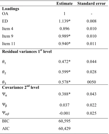
Different growth models were estimated in order to understand whether there was a significant change in the level of students’ satisfaction with the courses taught at the University of Padua in the academic years from 2012-2013 to 2014-2015. We started with a second-order unconditional growth model with a linear latent trajectory, i.e., a second-order growth model with five indicators (OA, ED, item 4, item 9, and item 11) and one underlying latent factor. We assumed loadings as time invariant. Table 8 lists estimation results: the residual variances of the latent construct (first-level) are significantly different from 0 indicating a lack of fit with the data. Even though the model must be improved, the estimates of the latent trajectory provide the evolution of the students’ evaluation of the didactics at the University of Padua in the three academic years of the reference period. According to the variances of the latent factors, the intercept and the slope of the model are uncorrelated. Only the intercept has a variance significantly different from 0, as shown by the estimates of the covariance of the second-level component of the model; this means that there are differences in the initial level of students’ satisfaction in the sample of didactic activities but that there is a non-significant different evolution over time.

12

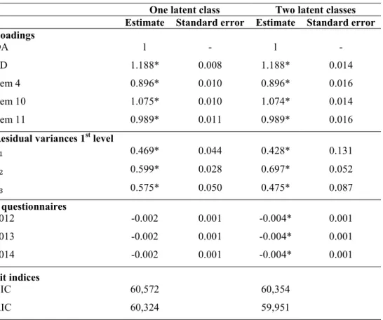
The general specification defines the mixture growth model with covariates, i.e., specifying conditional models. Table 9 compares the estimates obtained with the two conditional models: one-component mixture models (𝐾 = 1) and two-component mixture model (𝐾 = 2)4_{. Again, we considered factor loadings as invariant over time and over the two}

classes in the case of the mixture model. Type of degree, school, the position of the teacher, the fact that the course is an elective offered by a different degree course, and the number of hours taught5 _{have been considered as potential}

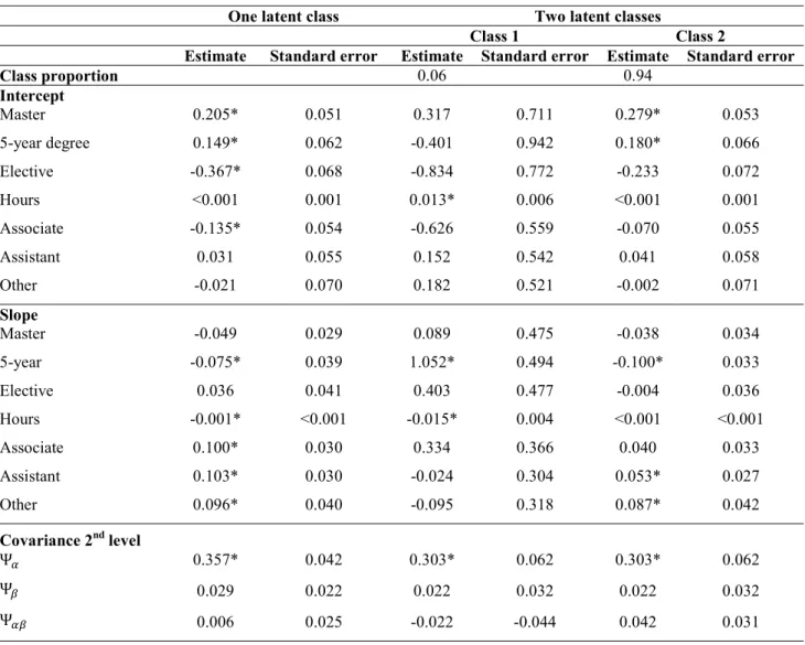
covariates for the latent intercept and slope and of the two latent classes. Table 10 lists the results only for those covariates that showed a significant effect either on the intercept or the slope; for categorical variables, the level missing in the table is the reference category. The number of filled-in questionnaires, the only time-varying variable, has been included in the model as a potential covariate for the latent factor; it shows a significant effect only in the two-class model (Table 9).

==== Table 9 about here ====

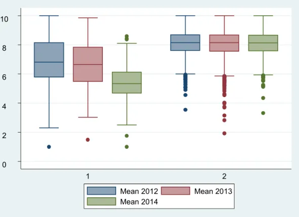
The measurement component of the two models under comparison is not very different; in the case of two classes, standard errors of estimates are only slightly higher (Table 9). The conditional latent growth mixture model shows a better fit to the data according to the AIC and BIC indices. The two unobservable classes of didactic activities have very different sizes. In the smallest group (6%, 114 courses)6_{, the average level of satisfaction is lower (Figure 2). It is}

interesting to note that the only time-varying covariate, which is the average number of filled-in questionnaires, has a significant negative effect on the mixture model. This effect (parameter) is assumed to be constant over classes and time. The estimated value shows that the number of students filling in the questionnaires, which is a proxy of the size of the audience of the course, has a negative effect on satisfaction.

==== Figure 2 about here ====

==== Table 10 about here ====

4 _{Three-component mixture models always perform worse than the two-component mixture model (based on BIC).} 5 _{The number of credits has been excluded from the potential covariates since it is highly correlated with the number}

of hours.

6 _{The classification is based on the estimates given by Equation 7 and assigned to the latent class with maximum}

probability (Bayes’ optimal rule). The relative entropy index, which varies between 0 (min) and 1 (max), is 0.908. Thus, we have a good level of separation of the mixture components (Ramaswany et al. 1993).

13

In the homogeneous conditional growth model, the type of the degree, the fact that the course is an elective from another degree and the position of the teacher significantly affect the intercept and the slope of the latent trajectory (Table 10). Courses in Master and 5-year degrees have a higher initial level of satisfaction than those in Bachelor degrees. The fact that the course is an elective from another degree has a negative impact on satisfaction in the academic year 2012-2013. Finally, courses taught by an associate professor have a lower initial level of satisfaction vis-a-vis those taught by full professors; however, satisfaction with courses not taught by a full professor improves over time. Finally, students’ satisfaction diminishes over time as the number of hours increases and in 5-year degrees. In the mixture conditional growth model, the number of hours has a positive and significant effect on the intercept in the smallest class, i.e., longer courses have a higher initial level of satisfaction but the number of hours has a significant negative effect on the slope, i.e., a decrease in satisfaction is estimated with an increase in the number of didactic activities. Moreover, in class 1 a significant positive effect is estimated on the slope in the case of courses belonging to 5-year degrees. In class 2, courses in Master and 5-year degrees have a higher initial level of satisfaction. There is a significant and positive effect on the slope when the teacher is other than full professor and a significant negative effect for 5-year courses.

Figure 2 contains the box plot of the mean obtained with the five indicators (Item 4, 10 and 11, OA and ED) in the two classes over the three academic years. The great majority of didactic activities in class 2 do not generally show variations in the level of students’ satisfaction over time and this level is higher with reference to all indicators. Didactic activities in class 1 (114 courses) clearly show a lower initial level of satisfaction and its decline over the academic years.

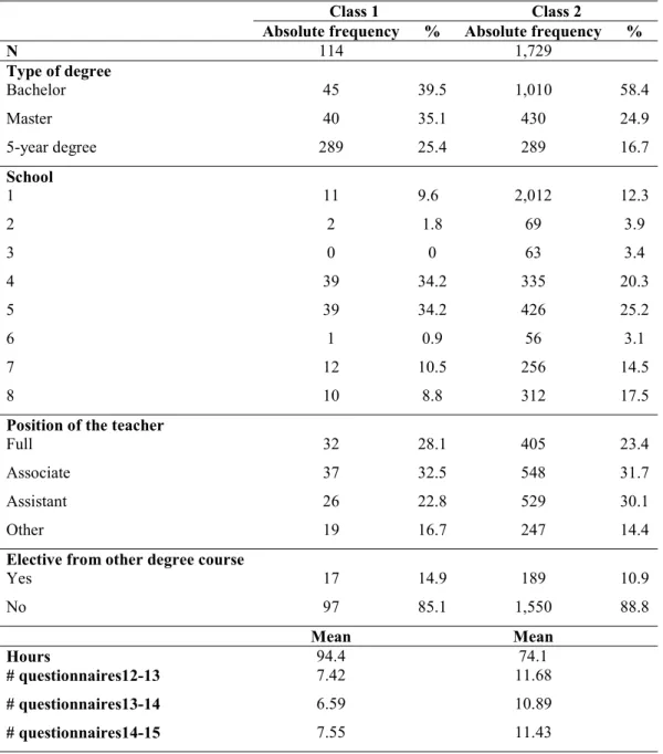
The estimation of the mixture conditional growth model allows us to isolate a small group of problematic didactic activities with lower assessments by students in the academic year 2012-2013 and with no improvement in the quality of these activities in the subsequent academic years. Table 11 compares the two classes of courses with the characteristics available in our database. In class 1, we find a higher proportion of didactic activities in Master and 5-year degrees, taught by full professors, electives from other degrees, with a higher average number of hours and, consequently, credits; in class 1, the average number of questionnaires filled in by the students is lower in all three academic years. This last evidence suggests that students attend these courses less. The distribution across university schools is very different in the two classes. The type of degree, the school, the number of hours and the average number of filled-in questionnaires is significantly different in the two groups of courses. This result is confirmed by the concomitant component of the model (Equation 7) with prior probabilities as the dependent variable (Class 2 is the reference category, Table 12).

14

==== Table 11 about here ==== ==== Table 12 about here ==== 5. Discussion

In this paper, we estimate a multiple-indicator growth mixture model on SET educational records regarding students’ satisfaction with teaching at university. The model tracks students’ satisfaction with the didactics of courses at a large Italian university. The case study uses data collected from questionnaires to measure students’ satisfaction over three consecutive academic years. Only items that were repeated measures in the questionnaire for all the three years were selected for courses that maintained the same characteristics such as the number of class hours and the teacher. Our goal was to develop a model able to track outlier didactic activities for which the patterns in the evolution of students’ assessments over time are very different from the average. Additionally, the outlier didactic activities identified can be associated with covariates that cause the specific dynamics over time and require managerial intervention.

The proposed latent growth mixture model contains three-components: a factor-analytic component that defined the measurement model based on five indicators (items 4, 9, 11, and indictors OA and ED); the latent growth component that models the dynamics of the latent trajectory; and the mixture component, which identifies the outlier group and conditionally includes covariates that affect growth factors and class membership.

The mixture model is able to identify a small group of problematic courses that not only have a low initial level of satisfaction but also a declining level of satisfaction over time in the three academic years under analysis. The majority of the examined didactic activities seem to go well with a high average satisfaction rate at the start of the observation period (almost 8 on a scale from 1 to 10) and continuing with the same level over time. The model manages to separate these many good didactic activities from the small residual group of bad ones. The identification of these didactic activities is very important for the university in order to improve the overall quality of didactics. These didactic activities are characterized by a higher average number of hours of lessons and by the fact they are mostly electives from other degrees. Despite the non-significance of the covariate identifying the school in the concomitant component for class membership, the majority of problematic courses (almost 70%) belong to two specific schools. It is also revealing that some of the covariates are not important in tracking the outlier courses. The university management is provided with an overview of the quality of the didactics, the evolution over consecutive academic years and, at the same time, a clear picture of didactic activities that are underperforming and require intervention.

15

The proposed model proves to be a very useful instrument to identify problematic aspects in the service industry even in a context, as in this large university, where client (student) satisfaction is on average high. Unlike other traditional frameworks, this framework integrates the different components from the pre-selection of items up to the identification of outlier services and factors explaining that behavior. Its implementation involves a combination of data reduction and clustering (unsupervised) methods.

This approach permits the introduction of covariates in the model that describe the characteristics of customers or the service. Regarding specific applications, it may be useful to consider richer databases that include the teacher’s characteristics, such as age or gender, and the composition of the course, among others (Spooren et al. 2013). In particular, if the researcher has access to student-level data (instead of averaged items per course), a more detailed analysis can be made using, for example, multilevel structures with students within courses.

As there was no individual data, we ran models assuming metric observed data; alternatively, a nonmetric specification such as Item Response Theory (IRT) could have been applied (van der Linden and Hambleton 1997; Bartolucci et al. 2015), which would have allowed the identification of students with outlier patterns of change instead. If data aggregation at class level retains frequency of scores (not just the arithmetic mean), a specification of the measurement model similar to Bacci et al. (2017) is advised. Where more waves are available, the model could be extended to define more complex residual structures of the model. In particular, measurement values of the items may not be totally explained by the latent trajectory and an error correlation structure can be specified (Grilli and Varriale 2014, Grimm and Widaman 2010). Another possible model specification could define specific trajectories to the items and avoid the need for covariances between residuals (Bishop et al. 2015).

References

Akaike, H. (1974). A new look at statistical-model identification. IEEE Transactions on Automatic Control, AC19(6), 716-723.

Alves, B. C., & Dias, J. G. (2015). Survival mixture models in behavioral scoring. Expert Systems with Applications, 42(2), 3902-3910.

Bacci, S., Bartolucci, F., Grilli, L. & Rampichini, C. (2017). Evaluation of student performance through a multidimensional finite mixture IRT model. Multivariate Behavioral Research, 52(6), 732-746.

Baker, R. S. (2014). Educational data mining: An advance for intelligent systems in education. IEEE Intelligent Systems, 29(3), 78-82.

Bartholomew, D. J., & Knott, M. (1999). Latent Variable Models and Factor Analysis. London: Arnold.

Bartolucci, F., Bacci, S., & Gnaldi, M. (2015). Statistical Analysis of Questionnaires: A Unified Approach based on R and Stata. London: Chapman and Hall/CRC.

16

Bartolucci, F., Farcomeni, A., & Pennoni, F. (2012), Latent Markov Models for Longitudinal Data, Boca Raton: Chapman & Hall/CRC.

Bassi, F. (2010). Experiential goods and customer satisfaction: An application to movies. Quality Technology & Quantitative Management, 7(1), 51-67.

Bassi, F. (2016), Dynamic segmentation with growth mixture models. Advances in Data Analysis and Classification, 10(2), 263-279.

Bassi, F., Clerici, R. & Aquario, D. (2017). Students’ evaluation of teaching at a large Italian university: measurement scale validation. Electronic Journal of Applied Statistical Analysis, 10(1), 93-117.

Baum, L. E., Petrie, T., Soules, G., & Weiss, N. (1970). A maximization technique occurring in statistical analysis of probabilistic functions of Markov chains, Annals of Mathematical Statistics, 41(1), 164-171.

Biemer, P. P. (2011), Latent Class Analysis of Survey Error. Hoboken, NJ: John Wiley & Sons.

Bishop, J., Geiser, C., & Cole, D. A. (2015), Modeling latent growth with multiple indicators: A comparison of three approaches, Psychological Methods, 20(1), 43-62.

Bollen, K. A., & Curran, P. J. (2006). Latent Curve Models: A Structural Equation Approach. Hoboken, NJ: John Wiley & Sons.

Boring, A., Ottoboni, K., & Stark, P. B. (2016). Student evaluations of teaching (mostly) do not measure teaching effectiveness. Retrieved from Science Open.

Braga, M., Paccagnella, M. & Pellizzari, M. (2014). Evaluating students’ evaluations of professors. Economics of Education Review, 41(C), 71-88.

Churchill, G. A. (1979). A paradigm for developing better measures of marketing constructs. Journal of Marketing Research, 16(1), 64-73.

Clogg, C. C. (1995). Latent class models. In G. Arminger, C. C. Clogg, & M. E. Sobel (Eds.), Handbook of Statistical Modeling for the Social and Behavioral Sciences (pp. 311-359). New York: Plenum Press.

Collins, L. M., & Lanza, S. T. (2010), Latent Class and Latent Transition Analysis: With Applications in the Social, Behavioral, and Health Sciences. Hoboken, NJ: John Wiley & Sons.

Connel, A. M., & Frey, A. A. (2006). Growth mixture modelling in developmental psychology: overview and demonstration of heterogeneity in developmental trajectories of adolescent antisocial behaviour. Infant and Child Development, 15(6), 609-621.

Dalla Zuanna, G., Bassi F., Clerici, R., Paccagnella, O., Paggiaro, A., Aquario D., Mazzuco C., Martinoia, S., Stocco, C., & Pierobon, S. (2015). Tools for teaching assessment at Padua University: role, development and validation. PRODID Project (Teacher professional development and academic educational innovation) (Report of Research Unit n.3). Padua: Department of Statistical Sciences, University of Padua.

Dayton, C. M., & Macready, G. B. (1988). Concomitant-variable latent class models, Journal of the American Statistical Association, 83(401), 173-178.

de Angelis, L., & Dias, J. G. (2014). Mining categorical sequences from data using a hybrid clustering method. European Journal of Operational Research, 234(3), 720-730.

Dempster, A. P., Laird, N. M., & Rubin, D. B. (1977). Maximum likelihood from incomplete data via the EM algorithm (with discussion). Journal of the Royal Statistical Society B, 39, 1-38.

17

Dias, J. G. (2006). Latent class analysis and model selection. In M. Spiliopoulou, R. Kruse, C. Borgelt, A. Nürnberger, & W. Gaul (Eds.), From Data and Information Analysis to Knowledge Engineering (pp. 95-102). Berlin: Springer-Verlag.

Dias, J. G. (2007). Model selection criteria for model-based clustering of categorical time series data: A Monte Carlo study. In R. Decker, & H. J. Lenz (Eds.), Advances in Data Analysis (pp. 23-23). Berlin: Springer.

Dias, J. G., & Ramos, S. B. (2014). The aftermath of the subprime crisis - a clustering analysis of world banking sector. Review of Quantitative Finance and Accounting, 42(2), 293-308.

Dias, J. G., & Vermunt, J. K. (2007). Latent class modeling of website users’ search patterns: implications for online market segmentation. Journal of Retailing and Consumer Services, 14(6), 359-368.

Dias, J. G., Vermunt, J. K., & Ramos, S. B. (2015). Clustering financial time series: new insights from an extended hidden Markov model. European Journal of Operational Research, 243(3), 852-864.

Esling, P. & Agon, C. (2012), Time series data analysis. ACM Computing Survey, 45(19), 12.

European University Association (2016). Quality Culture in European Universities: A Bottom up Approach. Brussels: EUA.

Fabrigar, L. R., Wegener, D. T., MacCallum, R. C., & Strahan, E. J. (1999). Evaluating the use of exploratory factor analysis in psychological research. Psychological Methods, 4(3), 272-299.

Formann, A. K. (1992). Linear logistic latent class analysis for polytomous data, Journal of the American Statistical Association, 87(418), 476-486.

Frühwirth-Schnatter, S. (2006), Finite Mixture and Markov Switching Models, New York: Springer.

Goodman, L. A, (1974). Exploratory latent factor analysis using both identifiable and unidentifiable models. Biometrika, 61(2), 215-231.

Grilli, L., & Varriale, R. (2014). Specifying measurement error correlations in latent growth curve models with multiple indicators. Methodology: European Journal of Research Methods for the Behavioral and Social Sciences, 10(4), 117-125.

Grimm, K. J., & Widaman, K. F. (2010). Residual structures in latent growth curve modelling. Structural Equation Modeling, 17(3), 424-442.

Hagenaars, J. A., & McCutcheon, A. L. (2002). Applied Latent Class Analysis. Dordrecht: Kluwer Academic Publishers.

Harvey, L., & Green, D. (1993). Defining quality. Assessment and Evaluation in Higher Education, 18(1), 9-34. Hornstein, H. A. (2017). Student evaluations of teaching are an inadequate assessment tool for evaluating faculty

performance, Cogent Education, 4(1), 1-8.

La Rocca, M., Parrella, L., Primerano, I., Sulis, I, & Vitale, M.P. (2017). An integrated strategy for the analysis of student evaluation of teaching: from descriptive measures to explanatory models, Quality & Quantity, 51(2), 675-691.

Lazarsfeld, P. F., & Henry, N. W. (1968). Latent Structure Analysis. Boston: Houghton Mifflin.

Masserini, L., Liberati, C., & Mariani, P. (2017). Quality service in banking: a longitudinal approach. Quality & Quantity, 51(2), 509-523.

McArdle, J. J., & Epstein, D. (1987). Latent growth curves within developmental structural equation models. Child Development, 58, 110–133.

18

Meggiolaro, S., Giraldo, A., & Clerici, R. (2017). A multilevel competing risks model for analysis of university students’ careers in Italy. Studies in Higher Education, 42(7), 1259-1274.

Meredith, W., & Tisak, J. (1990). Latent curve analysis, Psychometrika, 55(1), 107-122.

Murias, P., de Miguel, J.C., & Rodríguez, D. (2008). A composite indicator for university quality assessment: The case of Spanish higher education system. Social Indicators Research, 89(1), 129-146.

Muthén, B. (2004). Latent variable analysis: Growth mixture modeling and related techniques for longitudinal data. In D. Kaplan (Ed.), Handbook of Quantitative Methodology for the Social Sciences (pp. 345–368). Newbury Park, CA: Sage Publications.

Muthén, B., & Shedden, K. (1999). Finite mixture modeling with mixture outcomes using the EM algorithm. Biometrics, 55(2), 463-469.

Nagin, D. S., & Land, K. C. (1993), Age, Criminal, careers, and population heterogeneity – specification and estimation of a nonparametric, mixed Poisson model, Criminology, 31(3), 327-362.

Nixon, E., Scullion, R., & Hearn, R. (20168). Her majesty the student: Marketised higher education and the narcissistic (dis)satisfactions of the student-consumer, Studies in Higher Education, 43(6), 927-943.

Pennoni, F., & Romeo, I. (2017). Latent Markov and growth mixture models for ordinal individual responses with covariates: a comparison. Statistical Analysis and Data Mining: The ASA Data Science Journal, 10(1), 29-39. Ramaswamy, V., Desarbo, W. S., Reibstein, D. J., & Robinson, W. T. (1993). An empirical pooling approach for

estimating marketing mix elasticities with PIMS data. Marketing Science, 12(1), 103-124.

Rampichini, C., Grilli, L., & Petrucci, A. (2004). Analysis of university course evaluations: from descriptive measures to multilevel models. Statistical Methods and Applications, 13, 357-373.

Schwarz, G. (1978). Estimating the dimension of a model. Annals of Statistics, 6, 461-464.

Spooren, P., Brockx, B., & Mortelmans, D. (2013). On the validity of student evaluation of teaching: the state of the art. Review of Educational Research, 83(4), 598-642.

Stroebe, W. (2016). Why good teaching evaluations may reward bad teaching: on grade inflation and other unintended consequences of student evaluations. Perspectives on Psychological Science, 1(86), 800-816.

Svinicki, M., & McKeachie, W. J. (2013). McKeachie’s Teaching Tips: Strategies, Research, and Theory for College and University Teachers. (13th _{ed.). Belmont, CA: Wadsworth.}

Theall, M., & Franklin, J. (2007). (Eds.) Student Ratings of Instruction: Issues for Improving Practice: New Directions for Teaching and Learning. San Francisco: Jossey-Bass.

Uttl, B., White, C. A., & Gonzalez, D. W. (2016). Meta-analysis of faculty’s teaching effectiveness: student evaluation of teaching ratings and student learning are not related. Studies in Educational Evaluation, 54, 22-42.

van de Pol, F., & Langeheine, R. (1990). Mixed Markov latent class models. Sociological Methodology, 20, 213-247. van de Pol, F., Mannan, H. (2002), Questions of a novice in latent Markov modelling, Methods of Psychological

Research Online, 7(2), 1-18.

van der Linden, W. J., & Hambleton, R. K. (1997), Handbook of Modern Item Response Theory, New York: Springer. Vermunt, J. K., Langeheine, R., & Bockenholt, U. (1999), Discrete-time discrete-state latent Markov models with

time-constant and time-varying covariates, Journal of Educational and Behavioral Statistics, 24(2) 179-207.

Wedel, M., & Kamakura, W. A. (2000). Market Segmentation: Conceptual and Methodological Foundations. Dordrecht: Kluwer Academic Publishers.

19

Weng, L.-J. (2004), Impact of the number of response categories and anchor labels on coefficient alpha and test-retest reliability, Educational and Psychological Measurement, 64(6), 956-972.

Wiggins, L. M. (1955). Mathematical Models for the Interpretation of Attitude and Behavior Change. Columbia University.

Wu, H., & Leung, S.-O. (2017), Can Likert scales be treated as interval scales? A simulation study, Journal of Social Service Research, 43(4), 527-532.

Zabaleta, F. (2007). The use and misuse of student evaluations of teaching. Teaching in Higher Education, 12, 55-76. Zucchini, W., MacDonald, I. L., & Langrock, R. (2016), Hidden Markov Models for Time Series: An Introduction using

20

21

Figure 2. Means obtained averaging the five indicators in the two classes over the three academic years 0 2 4 6 8 10 1 2 Mean 2012 Mean 2013 Mean 2014

22

Table 1. Filled-in questionnaires by percentage of class attendance and degree of the respondent, academic year 2012-2013.

Attendance Type of degree

Erasmus Bachelor Master 5-year-long Total

Non-attendant 19.2 6.4 12.6 7.8 7.9 Less than 30% 6.3 3.0 2.8 2.3 2.9 Between 30 and 50% 9.5 4.8 4.2 3.4 4.5 Between 50 and 70% 18.9 11.3 11.4 10.0 11.2 More than 70% 46.1 74.5 69.1 76.5 73.4 Total number 3,496 124,445 33,548 34,614 196,103

23

Table 2. Number of didactic activities evaluated and average number of filled-in questionnaires by degree of respondent, academic year 2012-2013.

Bachelor Master 5-year-long Total

Number of activities 4,543 2,035 1,889 8,467

With at least 15 filled-in questionnaires 2,408 (53%) 783 (38%) 664 (35%) 3,855 (46%)

Average number of filled-in questionnaire

24

Table 3. Descriptive statistics of the assessed didactic activities

Absolute frequency % Type of degree Bachelor 1,064 57.4 Master 471 25.4 5-year-long 319 17.2 School 1 223 12.0 2 71 3.8 3 63 3.4 4 376 20.3 5 472 25.5 6 57 3.1 7 269 14.5 8 323 17.4

Position of the teacher

Full 437 23.6

Associate 585 31.6

Assistant 555 29.9

Other 277 14.9

Elective from other degree course

Yes 207 11.2

No 1,647 88.8

Mean Standard deviation

Hours 75.6 43.0

ECTS 8.0 2.4

# questionnaires12-13 11.4 11.3

# questionnaires13-14 10.6 10.0

25

Table 4. Descriptive statistics of the items

Item Mean 2012 St. dev. 2012 Mean 2013 St. dev. 2013 Mean 2014 St. dev. 2014

Item 1 8.14 1.06 8.00 1.15 7.95 1.22 Item 2 8.17 1.06 8.04 1.17 8.03 1.18 Item 3 8.33 1.05 8.24 1.13 8.21 1.10 Item 4 7.60 1.07 7.70 1.17 7.68 1.17 Item 5 8.18 1.04 8.16 1.12 8.09 1.18 Item 6 7.89 1.22 7.86 1.31 7.83 1.34 Item 7 7.85 1.25 7.85 1.32 7.81 1.34 Item 8 7.77 1.15 7.77 1.24 7.75 1.27 Item 9 8.30 1.07 8.18 1.16 8.09 1.22 Item10 7.98 1.12 7.86 1.27 7.83 1.29 Item11 7.61 1.17 7.62 1.26 7.61 1.29 Item12 7.86 1.17 7.88 1.24 7.80 1.29 Average over first 11 items 7.98 0.97 7.93 1.07 7.90 1.11

26

Table 5. Results of the exploratory factor analysis

Item Loading Item-to-rest Cronbach alpha

Item 1 0.942 0.927 0.972 Item 2 0.904 0.882 0.973 Item 3 0.863 0.835 0.974 Item 4 0.843 0.812 0.975 Item 5 0.880 0.854 0.974 Item 6 0.940 0.924 0.972 Item 7 0.935 0.919 0.972 Item 8 0.936 0.920 0.972 Item 9 0.890 0,867 0.974 Item10 0.897 0.874 0.973 Item11 0.836 0.804 0.975

27

Table 6. Results of the confirmatory factor analysis

Item Intercept Standard

Error Slope Standard Error

Item 1 0.941* 0.003 6.535* 0.110 Item 2 0.889* 0.005 6.787* 0.114 Item 3 0.832* 0.007 7.435* 0.124 Item 4 0.818* 0.008 6.560* 0.110 Item 5 0.868* 0.006 6.851* 0.115 Item 6 0.947* 0.003 5.850* 0.099 Item 7 0.947* 0.003 5.842* 0.099 Item 8 0.934* 0.003 6.102* 0.103 Item 9 0.865* 0.006 6.638* 0.111 Item 10 0.880* 0.005 6.060* 0.102 Item 11 0.806* 0.100 5.911* 0.100

28

Table 7. Goodness of fit indices for the full and the reduced models

Index Full model Reduced model

LR (df) 2,072.765(44) 69,823(5) RMSEA 0.158 0.084 Prob RMSEA < 0.05 0.000 0.001 AIC 50,560.152 20,526.883 CFI 0.927 0.993 TLI 0.909 0.987 SRMR 0.026 0.012 CD 0.981 0.967 Cronbach’s alpha 0.976 0.949 AVE 0.785 0.790 CR 0.976 0.949

29

Table 8. Unconditional second-order growth model: estimation results Estimate Standard error

Loadings OA 1 - ED 1.139* 0.008 Item 4 0.896 0.010 Item 9 0.989* 0.010 Item 11 0.940* 0.011

Residual variances 1st _level

𝜃 0.472* 0.044 𝜃 0.599* 0.028 𝜃 0.578* 0050 Covariance 2nd _level Ψ 0.388* 0.043 Ψ _{0.037 0.022} Ψ -0.001 0.025 BIC 60,595 AIC 60,429 Note: * p-value <0.001.

30

Table 9. Conditional second-order growth model: estimation results in the case of homogeneity and of two latent classes – measurement component

One latent class Two latent classes

Estimate Standard error Estimate Standard error Loadings OA 1 - 1 - ED 1.188* 0.008 1.188* 0.014 Item 4 0.896* 0.010 0.896* 0.016 Item 10 1.075* 0.010 1.074* 0.014 Item 11 0.989* 0.011 0.989* 0.016

Residual variances 1st _level

𝜃 0.469* 0.044 0.428* 0.131 𝜃 0.599* 0.028 0.697* 0.052 𝜃 0.575* 0.050 0.475* 0.087 # questionnaires 2012 -0.002 0.001 -0.004* 0.001 2013 -0.002 0.001 -0.004* 0.001 2014 -0.002 0.001 -0.004* 0.001 Fit indices BIC 60,572 60,354 AIC 60,324 59,951 Note: * p-value <0.001.

31

Table 10. Conditional second-order growth model: estimation results in the case of homogeneity and of two latent classes – structural component

One latent class Two latent classes

Class 1 Class 2

Estimate Standard error Estimate Standard error Estimate Standard error

Class proportion 0.06 0.94 Intercept Master 0.205* 0.051 0.317 0.711 0.279* 0.053 5-year degree 0.149* 0.062 -0.401 0.942 0.180* 0.066 Elective -0.367* 0.068 -0.834 0.772 -0.233 0.072 Hours <0.001 0.001 0.013* 0.006 <0.001 0.001 Associate -0.135* 0.054 -0.626 0.559 -0.070 0.055 Assistant 0.031 0.055 0.152 0.542 0.041 0.058 Other -0.021 0.070 0.182 0.521 -0.002 0.071 Slope Master -0.049 0.029 0.089 0.475 -0.038 0.034 5-year -0.075* 0.039 1.052* 0.494 -0.100* 0.033 Elective 0.036 0.041 0.403 0.477 -0.004 0.036 Hours -0.001* <0.001 -0.015* 0.004 <0.001 <0.001 Associate 0.100* 0.030 0.334 0.366 0.040 0.033 Assistant 0.103* 0.030 -0.024 0.304 0.053* 0.027 Other 0.096* 0.040 -0.095 0.318 0.087* 0.042 Covariance 2nd _level Ψ 0.357* 0.042 0.303* 0.062 0.303* 0.062 Ψ 0.029 0.022 0.022 0.032 0.022 0.032 Ψ 0.006 0.025 -0.022 -0.044 0.042 0.031 Note: * p-value <0.001.

32

Table 11. Didactic activities in the two classes of the mixture conditional growth model by characteristic

Class 1 Class 2

Absolute frequency % Absolute frequency %

N 114 1,729 Type of degree Bachelor 45 39.5 1,010 58.4 Master 40 35.1 430 24.9 5-year degree 289 25.4 289 16.7 School 1 11 9.6 2,012 12.3 2 2 1.8 69 3.9 3 0 0 63 3.4 4 39 34.2 335 20.3 5 39 34.2 426 25.2 6 1 0.9 56 3.1 7 12 10.5 256 14.5 8 10 8.8 312 17.5

Position of the teacher

Full 32 28.1 405 23.4

Associate 37 32.5 548 31.7

Assistant 26 22.8 529 30.1

Other 19 16.7 247 14.4

Elective from other degree course

Yes 17 14.9 189 10.9 No 97 85.1 1,550 88.8 Mean Mean Hours 94.4 74.1 # questionnaires12-13 7.42 11.68 # questionnaires13-14 6.59 10.89 # questionnaires14-15 7.55 11.43

33

Table 12. Effect of concomitant variables on priori probabilities Estimate Standard error

Type of degree

Master 1.089* 0.446

5-year degree 0.401 0.537

Hours 0.008* 0.003