N UMERICALA LGORITHMS FOR THEV ALUATION OFI NSTALLMENT O PTIONS S OFIAS ANDE DEA RAÚJO

M

ESTRADO

M

ATEMÁTICA

F

INANCEIRA

T

RABALHO

F

INAL DE

M

ESTRADO

D

ISSERTAÇÃO

N

UMERICAL

A

LGORITHMS FOR THE

V

ALUATION OF

I

NSTALLMENT

O

PTIONS

S

OFIA

S

ANDE DE

A

RAÚJO

M

ESTRADO

M

ATEMÁTICA

F

INANCEIRA

T

RABALHO

F

INAL DE

M

ESTRADO

D

ISSERTAÇÃO

N

UMERICAL

A

LGORITHMS FOR THE

V

ALUATION OF

I

NSTALLMENT

O

PTIONS

S

OFIA

S

ANDE DE

A

RAÚJO

O

RIENTAÇÃO

:

MARIA

DO

ROSÁRIO

LOURENÇO

GROSSINHO

2

Contents

1 Introduction... 5

2 Literature Review ... 6

3 Theoretical Framework ... 7

4 Numerical Methodology ... 25

4.1 Prior Methods ... 25

4.2 The De Hoog algorithm ... 28

5 Computational Results ... 29

6 Conclusions... 37

3

Acknowledgments

First and foremost, I would like to express my sincere gratitude to my advisor Prof. Maria do Rosário Grossinho for the continuous support of my thesis, for her motivation, enthusiasm and great knowledge.

Besides my advisor, I would like to thank the rest of my thesis committee: Prof. Onofre Alves Simões and Prof. Fernando Gonçalves for their encouragement and instructive comments and questions.

Last but not the least I would like to thank my family for supporting me throughout all my studies at University, my friends for their support and encouragement and my fiancé for his personal support and great patience at all times.

4

Abstract

Installment options are financial derivatives in which part of the initial premium is paid up-front and the other part is paid discretely or continuously in installments during the option’s lifetime.

This work deals with the numerical valuation of European installment options. Trough the study of the continuous case, we can show that numerical inversion of Laplace transform works well for computing the option value. In particular, we will investigate the De Hoog algorithm and compare it to other methods for the inverse Laplace transformation, namely Euler summation, Gaver-Stehfest and Kryzhnyi methods.

Keywords: Installment options, compound options, Laplace transform, numerical inversion, stopping boundaries, De Hoog algorithm

Resumo

Installment options são derivados financeiros cuja parte inicial do prémio é paga antecipadamente e a outra parte é dividida, discretamente ou continuamente, em parcelas durante o “tempo de vida” do contrato.

Este trabalho estuda a valorização numérica de installment options do tipo Europeu. Estudando principalmente o caso contínuo podemos mostrar que a inversão numérica da transformada de Laplace é um bom método para calcular o valor da opção. Em particular, vamos investigar o algoritmo conhecido por De Hoog e compará-lo a outros métodos numéricos, sendo eles conhecidos por Euler summation, Gaver-Stehfest e método de Kryzhnyi.

5

1

Introduction

Derivatives have been cited as a key factor behind the 2008 financial crisis due mainly to their complexity and lack of transparency that caused capital markets to undervalue credit risk. Options enjoyed great popularity within this class of financial assets and a particular type of options has recently emerged: the installment option. Unlike most basic derivatives, installment options present a valuation challenge as analytical methods like the Black-Scholes model are unable to offer a closed solution; therefore, a numerical approach is required.

There are a number of alternatives in solving the valuation problems of this type of options. The best practice known so far is to apply the Laplace transform method and then use numerical algorithms to invert it. Kimura [21] had success on valuating these options numerically using Euler-summation and Gaver-Stehfest methods; the Kryzhnyi method was additionally tested by Ehrhardt et al. [14].

The main goal of this work is to test a new method known as the De Hoog algorithm and compare it to the previous methods. This algorithm is a Fourier Series Expansion [6,13] that uses an acceleration algorithm for its quotient-difference and has proven to be suitable for the long time integration of dissipative equations. In fact, and regarding the computational results, it appears to be the best candidate to valuate these options numerically.

Please note that some parts of this work follow closely the work of Kimura [21].

6

2

Literature Review

There has not been much research on installment options, mainly because it is an recent topic. The first publication was an article by Karsenty and Sikorav [20]. Davis et al. [9,8] derive no-arbitrage bounds for the initial premium of an installment option, which are used not only to set up static hedges but also to compare them with dynamic hedging strategies within a Black–Scholes framework considering stochastic volatility. Also, it concerns the European discrete installment options only, allowing an analogy with compound options, as covered by Geske [16] and Hodges and Selby [19]. Ben-Ameur et al. [3] develop a dynamic programming procedure to price American discrete installment options and investigate some theoretical properties of the installment option contract regarding the geometric Brownian motion. Griebsch et al. [18] deduce a closed form solution to the initial premium of a European discrete installment option in terms of multidimensional cumulative Normal distribution functions. When examining the limiting case of an installment option with a continuous payment plan, it is found to be equivalent to a portfolio consisting of a European vanilla option and an American put on this vanilla option with a time-dependent strike. Kimura and Kikuchi [22] develop a valuation of installment options based on the Laplace transform while Ciurlia and Roko [4] apply the multipiece exponential function (MEF) method to define an integral form of the value of an American option. However, this method is critically restricted since it generates a discontinuity in the optimal stopping and early exercise boundaries.

7

3

Theoretical Framework

While in a conventional option contract the buyer pays the total premium up-front and acquires the right, but not the obligation, to exercise the option at maturity (European type) or at any time until maturity (American type), in an installment option the buyer pays a lower up-front premium, paying its remaining part in a series of “installments” or further premium payments, to be paid during the lifetime of the option up to maturity. At each installment date the holder has the right to decide if he continues to pay for the contract or he terminates the payments, in which case the option lapses with no further payments on either side. The opportunity to end the contract at any time before maturity turns the valuation of these options into a free boundary problem.

There are two cases of the installment payments: discrete and continuous.

An installment option with payments at pre-specified dates is usually referred to as a “discrete-installment option”.

The continuous case means that the holder pays a stream of the installments at a given rate per unit time. It is like accumulating the premium sum by a certain continuous rate that will be paid by the holder in the case of exercising.

Installment options will appeal to investors who are willing to pay a little extra for the opportunity to terminate payments and reduce losses if their investment position is not working out. They have been traded actively in actual markets as they have significant advantage over other options: the prevention of losses through possibility of termination; the low initial premium that is easy to schedule in the firm’s budget, etc. Typically these options are traded in Foreign Exchange markets between banks and corporates. Also, many life insurance contracts and capital investment projects can be thought of as installment options (cf. Dixit and Pindyck [11]).

8 In general, the compound option is a particular case of an installment option. Alobaidi et al. [1], Davis et al. [9] and others have mentioned that in the case of two discrete installment payments, we have a compound option, or in other words, an option on an option.

Note that the compound options were the initial point for further study of installment options. In fact, these two types of options look rather similar, so it is important to distinguish between them.

A compound option is an option on an option and as a consequence it has two strike prices and two expiration dates. In the moment of buying the compound option, the holder pays the initial premium and on the first expiration date he can choose either to buy the option or not. At this time the compound option turns into a European vanilla option which can be exercised or not on the second expiration date. Note that the initial price of the compound options is obviously smaller than the vanilla option price since the premium is split over time.

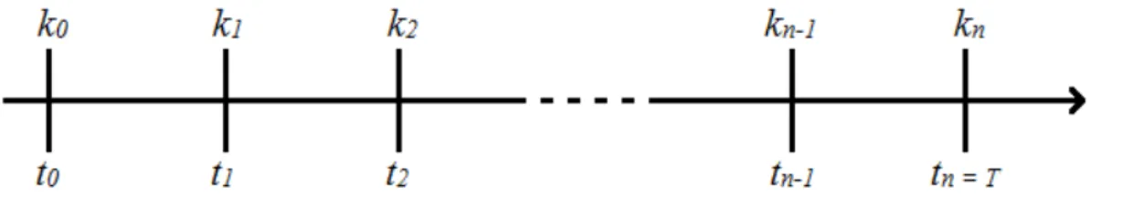
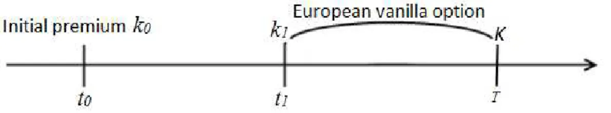
Figure 2.1: The lifetime of a compound option. t₀is the inception date, t₁ is the first expiration date, T is the time of maturity, k₀ is the initial premium, k₁is the first strike price, Kis the strike price at the time of maturity.

For both compound and installment options we have that their total premium is always higher than the price of the standard ones. This is explained by the additional right to terminate the contract without paying the whole sum of the premium.

9 option on an option and so on. Each fold option may be either call or put. Actually a multi-fold compound option is nothing else than the discrete installment option, although the first published paper devoted to this type of options was written later in 1993 by Karsenty and Sikorav [20].

10

The Black-Scholes Pricing Model

We will now briefly describe the valuation of discrete installment options and for the continuous case we will define the problem of valuating European installment options. The setup is a standard Black–Scholes framework where the price of the underlying asset evolves according to a geometric Brownian motion.

First consider the discrete case. Let S_tbe the price of the underlying asset following a geometric Brownian motion described by the stochastic differential equation (SDE)

(3.1)

where 



r 



,ris the constant risk-free rate and  _{denotes the continuous} dividend yield.  Is the volatility coefficient of the asset price and dW_t is a standard Brownian motion on a risk-neutral probability space.

As we can see in Figure 3.1, t₀is the initial date and k₀ is the initial premium equal to the initial value of the option, V₀. The discrete installment option has n installment

dates t₁,...,tn. At each of these dates, the holder has to pay the premium k k1, 2..,kn1in order to continue the contract.

We want to compute the initial value of the installment option to enter the contract. We know that the option payoff at the time of maturity T is given by

t t t t

dS S dtS dW









max ,0

n n n

V   s k

11 where sS_T is the price of the underlying asset at T, k_n is the strike price and, as usual, _n  1for the underlying vanilla call option and _n  1 for a put option. At time t_n1 the option value is given by the discount expectation of the value V_n. Repeating this procedure, we can define the payoff function of this option.

We also know that at time t_i the holder can stop paying the premiums, terminating the contract, or pay k_i to continue.

In the case of continuation, the value of the option at time t_i is given by the backward recursion

(3.2)

Thus, the unique arbitrage-free price of the installment option is

 

1 0

 

1 0

0 0 1 .

r t t

t t V s k e  _V S S s_

Using the Curnow and Dunnet integral reduction technique to solve (3.2), a closed-form solution to valuate the installment option was derived (cf. Griebsch et al. [18] for details).

There are other methods to valuate discrete installment options (cf. Ben-Ameur et al. [3]) but in comparison to them the presented closed-form formula seems to be the most suitable way to do that.

Consider now the continuous case. Let S_t be the price of the underlying asset following a geometric Brownian motion described by the stochastic differential equation (SDE) described in (3.1).

The Black-Scholes initial premium Vof a continuous installment option

(3.3) depends on the time t, the current value of the underlying asset St, and the

continuous installment rate q. In time dtthe premium qdthas to be paid to stay in the option contract.



, ,



t t

V V t S q

 



 

 



 

1

1

1

max , 0 for 1,..., 1

for

i i

i i

r t t

i t t i

i

n

e V S S s k i n

V s

V s i n





 



 _{    }

 _{ }

 

 

12





2 2 2

2 1

. 2

t t t t

t t t t t

V V V V

d r S q S dt S dW

S t S S

             _  _   _     _  _  _          

Applying Itô’s Lemma to (3.3) we obtain the dynamics for the option’s initial value

(3.4)

We now construct a portfolio consisting of one option and an amount  of the underlying asset

t Vt St

   

and its dynamics is given by

(3.5)

Plugging (3.1) and (3.4) into (3.5) we obtain

To turn this portfolio riskless we choose   V_t S . Also, to avoid arbitrage opportunities the portfolio has to yield the returnr, so we must have

Finally, by rearranging this equation, we obtain an inhomogeneous Black-Scholes partial differential equation (PDE) for the initial premium of this option

(3.6)

We should have q greater than zero. If it is equal to zero then we get the homogeneous Black-Scholes PDE.

The Call case

Consider a European-style installment option with maturity date Tand strike priceK. Let cc t S q



, ;_t



denote the value of this call option at time t defined on the domain

 

   



t S, _t 0,T 0,



   

D

.





2 2 2

2 1

2

t t t t

t t t t

V V V V

dV r S q dt S dW

t  S  S  S

    

_     _ 

   

 





.

t t t t

d dV  dS   S dt





2 2 2

2

1

. 2

t t t

t t t

V V V

r S S rV q

t  S  S

           2 2 2 2 1 . 2

t t t t

t t t t

V V V V

r V S S q S

S t  S S 

13 The payoff at the maturity is max



S_TK, 0



. The additional opportunity to end the contract at any time t

 

0,T turns the valuation of continuous installment options into an optimal stopping problem. This is equivalent to finding the points



t S, _t



for which the termination of the contract is optimal.

Let

S

_and

C

_{denote the} stopping region and continuation region respectively. The stopping region is defined in terms of the value function c t S q



, ;_t



by

 







t S, t c t S q, ;t 0



  

S

D

for which the optimal stopping time *

c

 satisfies

 









*

inf , ,

c u t T u Su

   

S

.

Since the continuation region

C

is the complement of

S

in

D

, we have

 







t S, t  c t S q, ;t 0



= D

C

.

The boundary that lies between regions

S

and

C

is called stopping boundary and is defined by

 









 

inf 0, , ; 0 , 0,

t t t

S  S   c t S q  t T .

Since c t S q



, ;_t



is no decreasing inS_t, the stopping boundary

 

_{ }

0,

t t T

S _ is a lower critical asset price below which it is convenient to terminate the contract by stopping the payments.

In the continuation region

C

_{the value} c t S q



, ;_t



is obtained by solving the inhomogeneous PDE

with the boundary conditions

and the terminal condition





2 2 2

2 1

,

2 t

c c c

r S S rc q S S

t  S  S

 _{ }  _  _{  }

  





lim , ; 0, lim 0, lim

t t

S S S S S

c c

c t S q

S S

  

 

   

14





 













 

12

2

2 1 2 1

2 1

log , ,

, , , ,

1

, z 2

z _v

a b r

d a b

d a b d a b

N z e dv

  



 

   

 



   

 



_





, ;



max



,0



c T S q  SK .

The following integral representation is the value function of the continuous installment call option



 



 









2

, ; , T r u t , ,

u

t t t

t

c t S q c t S q



e  N d S S u t du (3.7)

where

and c t S



, _t

 

c t S, ;0_t



is the value of the European vanilla call option





 



_

_



 



_

_



1 2

, _{t t} T t _t, , r T t _t, ,

c t S S e  N d S K Tt Ke  N d S K Tt .

This proof is given in the work of Kimura [21].

From (3.7) we can easily see that the price of the continuous installment option is the difference between the corresponding European vanilla call option and the expected present value of the installment premiums along the optimal stopping boundary. Also from (3.7) we immediately see that c t S q



, ;_t

 

c t S, _t



for t

 

0,T , which means that the payment of installment makes the initial premium lower than the vanilla counterpart.

Furthermore, the optimal stopping boundary

 

_{ }

0,

t t T

S _ is implicitly defined by the following integral equation





 



_

_



2

, t T r u t t, u, 0

t

c t S q



e  N d S S u t du 

which can be solved numerically for

 

_{ }

0,

t t T

15 However, in the current work, to find the values of options and, therefore, the optimal stopping boundaries, we consider an alternative approach based on Laplace transforms, which generates the transformed stopping boundary in a closed-form. Regarding that we will present the Laplace-Carson transformation method and inverse Laplace transformation methods.

The Put case

We proceed the same way for the valuation of a continuous installment put option. Its value at time tis defined by p p t S q



, ;_t



on the same domain

D

.

For each time t

 

0,T there exists an upper critical asset price above which it is advantageous to terminate payments by stopping the option contract.

The stopping boundary also divides the domain

D

into a continuation region

 

 





t S, t  0,T  0,St



=

C

and a stopping region

 

 



t S, _t 0,T S_t,



  _ _

S

.

The value p p t S q



, ;_t



satisfies the inhomogeneous Black-Scholes PDE in the continuation region

C

, i.e.

subject to the following boundary and terminal conditions

Again, as in Kimura [21], the value function of the continuous installment put option is represented by the following integral









 









2

, _t; , _t T r u t _t, _u,

t

p t S q  p t S q



e  N d S S u t du (3.8)





2 2 2

2 1

,

2 t

p p p

r S S rp q S S

t  S  S

  

     

  













0

lim , ; 0, lim 0, lim

, ; max , 0

t t

S S S S S

p p

p t S q

S S

p T S q K S

  

 

   

 

 

16 where p t S



, _t



p t S



, _t;0



is the value of the European vanilla put option

 

 



_

_



 



_

_



2 1

,

_t r T t _t

, ,

_t T t _t

, ,

p t S



Ke

 

N



d S K T t

 

S e

 

N



d S K T t



.

A decomposition of the total Premium

To understand the original idea of the decomposition of the total premium let us return to the subject of the compound options.

Davis et al. [9] recommended an alternative way of looking at the compound call on a call option. Actually, the price of the underlying call to be paid at time t₀ is the amount

1 0

0 1

r t t

k k k e  , i.e., the sum of the initial premium and the discounted value of the second premium. At the same time, the holder has the right to get rid of this option and selling it for the price k₁ at timet₁. Hence, the total premium of the compound call on a call option can be viewed as the underlying call option plus a put on the call with exercise at time t₁ and strike pricek₁1

Following the same idea, suppose that the total premium of the installment option equals the underlying European vanilla call option plus the right to leave at any time at a pre-determined rate.

Griebsch et al. [18] proved this idea considering the limiting case of discrete installment options and the risk-neutral approach. They observed that the total premium of the continuous installment call option is the European vanilla call option plus an American put option on this European call



, _t;



_t



, _t



_c



, _t;



c t S q K c t S P t S q (3.9)

where

(3.10)

1

Here cBSt T S, , _t,K and BS , , , 

call t T St K

p denote a European vanilla call and put on a call option respectively, with a strike

price Kmaturity at T and underlying spot priceS_t

 



1 r T t



t

q

K e

r

 

 

1 0









0 0

0 1 0, , , call 0, ,1 , 1

r t t BS BS

t t

17 is the discounted sum of the premiums not to be paid if the holder decides to terminate the contract at time t, and for the set St T, of stopping times with values in

 

0,

t T





 



_

_



,

, ; ess sup max , , 0

t T

r u t

c t u S u u t

P t S q  _ _e  k c u S

F

_ a.s.

is the value of the American compound put option with the maturity at T written on the European vanilla call option.

This decomposition will be used to obtain the Greeks formulas showed later on.

The Laplace Transform

Nowadays integral transforms are a common practice to solve problems of the mathematical modeling.

Bateman [2] was the first to consider the Laplace transform as a tool for solving integral equations.

Definition 1: (Laplace transformation)

Assume that f t( )is a real valued function defined for all positive t in the range



0,



. Then the Laplace transform of the function f t( )is defined by





0

( ) t ( )

f t e  f t dt

  



L (3.11)

if the integral

0

( )

t

e  f t dt 





converges. The parameter  is a complex number.

Applying the Laplace transform to the Black-Scholes PDE (with two variables, time and asset price) will reduce it to an ordinary differential equation (ODE) with respect to the asset price, which is a much simpler problem.

18

Definition 2: (Laplace-Carson transformation)

For the same assumptions as above, the Laplace-Carson transform of the functionf t( ) is defined by





0

( ) t ( )

f t  e  f t dt

  

_

LC (3.12)

There is no essential difference between these two transformations, but the principal reason why LCT is used is that it generates relatively simple formulas for option pricing problems.

From Definition 2 it follows that for any two functions f t( ) and g t( ) satisfying the conditions of Definition 1 then

















0

( ) ( ) t ( ) ( ) ( ) ( )

af t bg t  e  af t bg t dt a f t b g t

 

 

_

  

LC LC LC (3.13)

Lemma 1: Assuming that f t( ) is continuous and differentiable and f t'( ) is continuous except at a finite number of points in any finite interval

 

0,T then



f t'( )







f t( )



f(0)

LC LC (3.14)

The proof can be viewed on Cohen [5].

The Inverse Laplace Transform

Denote by 1



 



F 



L the inverse Laplace transform for a functionF

 

 L



f t( )



, i.e.

 





1

( )

F  f t

 _

L

Note that for functions f t( )and g t( ) that only differ in a finite set of values of t, we have



f t( )



=

 

g t( )

L L .

19 Hence, for applying the Laplace transform to our problem we need to be in the area of uniqueness. This leads us to Lerch’s theorem.

Theorem 1: (Lerch’s theorem [5])

If for a continuous function f t( ) _{there exists a function} F such that

 

0

( ) , ,

t

F  e  f t dt  

 



_

 (3.15)

then there is no other function satisfying (3.15).

Now, if we have an ODE solution for the corresponding transformed PDE, and an exact formula for determining 1



 



F 



L we can easily produce a continuous solution for our PDE.

In general, there is an analytical formula for the Laplace transform inversion, called the Bromwich integral.

Theorem 2: (The Inversion theorem [5])

Let f t( )have a continuous derivative and let f t( ) aet where  and a are positive constants. Define F

 

 L



f t( )



for Re

 

  . Then

where c .

Note that this integral is too complex for computing directly, thus various numerical methods are applied for computing the function values from its Laplace transform.

The analytical expressions for transformed variables

Transformed option values

The next step is to apply the Laplace transform on our inhomogeneous Black-Scholes PDE described in (3.6) and solve it in the transformed variables. As usual, we first consider the call case.

1

( ) ( )

2

c i ut

c i

f t e F u du i



 

 

20





 

 

1 * 2 , , ,

S S K c S

S K

S S K

r          _     _{  }    





2 2 2 2

1

0, 0,

2

c c c

r S S rc S

S S                  

For convenience we revert the direction of time by changing the variable  T t and defining c



, ;S q

 

c T, ;S q

 

c t S q, ;



and S ST St for 0. From Definition 2 the Laplace-Carson transform (LCT) of these variables is as follows

Applying the LCT to (3.6) we will get an inhomogeneous ODE of the same order. But to solve an ODE of this type it is necessary to solve first the corresponding homogeneous ODE, so it makes sense to consider the transformation of the original Black-Scholes PDE for the vanilla options, where q is absent.

Lemma 1: Let *







 



, ,

c S LC c  S be the LCT of the associated vanilla call for the backward running process. Then

(3.16)

where for i1, 2 we have

and the parameters   1 1

 

1 and 2  2

 

0 depend on  and are two real

roots of the quadratic equation

Proof: The original proof can be found in [21].

After changing variables, the Black-Scholes PDE reads

(3.17)

 

3

1 2

1

i

i i

K r S

S r K                 _  _{ }      

















 

 

* 0 * 0 , ; , ; , ;

c S q c S q e c S q d

S S e S d                    





LC LC





2 2 2

1 1

0

2  r  2   r

 

_   _   

21 supplied with the boundary conditions

and the initial conditionc

 

0,S max



SK,0

 

 SK



.

After transforming equation (3.17) and using (3.13) and (3.14), we obtain a corresponding ODE

(3.18)

with the boundary conditions

Equation (3.18) is a linear homogeneous ODE of Euler-type and can be reduced to a linear ODE with constant coefficients by substituting y

S e and solved easily yielding (3.16).

Theorem 4: [21] If SS*,

(3.19)

otherwise *





, ; 0

c  S q  . The stopping boundary S*S*

 

 is given by

Proof: For S0,S*_ the result is obvious. In a similar way in the proof of Lemma 1, we obtain the ODE for *





, ;

c  S q as

(3.20)

with the boundary conditions

 

0

lim , 0, lim ,

S S

dc c t S

dS

    













2 * *

2 2 *

2

1

0, 0,

2

d c dc

S r S r c S K S dS dS             





* * 0

lim , 0, lim

S S dc c S dS      









2

* * 1

*

1 2

, ; , q S q

c S q c S

r S r

            _{ }    _{ } 

 

_



_



1 1 * 2 2 2 1 q S K K                   













2 * *

*

2 2 *

2

1

,

2

d c dc

S r S r c q S K S S dS dS             





* * * * *

lim , ; 0, lim 0, lim

S

S S S S

dc dc c S q

dS dS





22 It is straightforward that the solution for (3.20) is a sum of solutions for the homogeneous equation and a particular solution of the inhomogeneous equation. It can be easily seen that the second part of the formula for *





, ;

c  S q is a solution for the corresponding inhomogeneous ODE. For a detailed proof, cf. [21].

The same approach can be used for compute the solution for the put case. The following theorem formulates the result2.

Theorem 5: [21] If *

S

S ,

(3.21)

and *





, ; 0

p  S q  otherwise, where

The stopping boundary is given by

Transformed Greeks

Recall the decomposition of the total premium of the installment option. Kimura [21] showed that this decomposition of the option in a vanilla call option and an American compound option is very valuable when trying to approximate the Greeks of the installment options.

Using (3.9) and the integral representation (3.7) we obtain





 



_

_



2

, ; , ,

T r u t

u

t c t t

t

K P t S q q e



  N d S S ut du.

2

For continuous installment put options, Kimura prove theorems similar to the theorems used in the call case, via the same PDE/LCT approach. However, the properties of the stopping boundary for the put case are subtly different from the call case. See [21] for details.









1

* * 2

* 1 2

, ; ,

S

q S q

p S q p S

r r             _{ }      





 

 

1 * 2 , , , S K

S S K

r p S

S S K

         _{  }       _ 

 

_



_



1 2 * 2 1 2 1

S q K

23

q r



Substituting N z

 

 1 N

 

z and using (3.10) we obtain an integral representation for the American compound option





 

_

_

_

_

2

, ; , ,

T r u t

u

c t t

t

P t S q q e



  N d S S ut du.

Regarding the linearity of the LCT and using it on (3.9) we get for time-reversed values







c t S q, t;





 

Kt 



c t S q



, t;









P t S qc



, t;





LC LC LC LC

which is equivalent to













* * * *

, ; , _c , ;

c  S q K_ c  S P  S q .

From Theorem 4 we see that

Here, the inverse LCT of the term can be computed analytically

thus the transformed value of an American put on a call is

(3.22)

Hence, the Greeks ofc t S q



, t;



, i.e. delta, gamma and theta, can be expressed by

Greeks of the vanilla call and Greeks of the American put on a vanilla call with floating strike priceK_t.

where





2

* * 1

* 1 2

, ;

c

q S q

P S q K

r S r

            _{ }    _{ }   





1 0 1 LC T

r T t ru

t

q q

q e du e K

r r         _{  }  _   







2

* 1 * 1 2 , ; c q S

P S q

r S          _{ }   _{ }    

 

   

 

   

 

* * * 1 , ; , 2 1 , ; 2 ,

1 , ; , LC LC + LC c c c

c t S q c t S P

c t S q c t S P

r

c t S q c t S P

c S c S c qe                                 









 









 

























1 , 1 ,

1 1 2

,

, ,

, ,

, , , , , ,

2

c t S

c t S

r c t S

e d S K e

d S K S

Se

24 Using (3.22) we find explicit formulas for the transformed Greeks of American compound options.

Using the same arguments for the put case we get the integral representation





 



_

_



2

, ; , ,

T r u t

p t t u

t

S

P t S q q e



  N d S ut du

and its LCT given by

Once again we have

where and correspondingly





















2 * 2 * 2 * * 1 2 * 1 2 2 2 *

1 2 2

2 2 2 *

1 2

* * 1

* 1 2 1 0 1 1 0

, ; 0, ; , ; 0

LC LC LC c c c c c P c c P c

c c c

P

P P q S

S S r S S

P P q S

r

S S S S

P q S

P S q P S q P S q

r S                                 _{ }  _{ }        _{ }         _{ }  _{ }                  _ _      _{ }       _{ }    

 

   

 

   

 

* * * 1 , ; , 2 1

, ; 2 ,

1 , ; , LC LC + LC p p p

p t S q p t S P

p t S q p t S P

r

p t S q p t S P

p S p S p qe                                 









 









 

























1 , 1 ,

1 1 2

,

, ,

, ,

, , , , , ,

2

p t S

p t S

r p t S

e d S K e

d S K S

Se

d S K Se d S K rKe d S K            _{    }                      





















1 * 1 * 1 * * 1 2 * 1 2 2 2 *

1 2 1

2 2 2 *

1 2

* * 2

* 1 2 1 0 1 1 0

, ; 0, ; , ; 0

LC LC LC p p p p p P p p P p

p p p

P

S

S

S

P P q S

S S r S

P P _{q S}

r

S S S

P q S

P S q P S q P S q

r                             _{ }   _{ }   _{ }              _{ }   _ _   _{ }                 _ _      _{ }        





1

* 2 * 1 2 , ; p S q S

P S q

25

4

Numerical Methodology

4.1 Prior Methods

The Euler-summation method

The Fourier-Series method for numerically inverting Laplace transforms was first proposed by Dubner and Abate [12]. An acceleration technique that has proven to be effective in our context is Euler summation, proposed by Simon et al. [26]. This method is based on the Bromwich contour inversion integral, which can be expressed as the integral of a real-valued function of a real variable by choosing a specific contour. The method is described as follows (cf. C. O’Cinneide [24] for details) in dependence of the parametersA,l,mand n (e.g.A19,l1,m11 and n38)

1. Computea_k, k0,1, ,mn:

2 2

0 0

1,

2 , 2 2

A l A l

k k

A

a b k a b F

lt lt lt

e _ e   

  _{   }     where 1

2 Re 0

2 ,

l

ij l k

j

A ij ik

b F k

lt lt t e

            _{   }    



2. Compute

 

0

1 , 0, ,

j k

j k

k

s a j n m



  





_.

3. Approximate f t( )using

The Gaver-Stehfest method

Another way to represent the inverse transform is given in the following result of Post and Widder [25,28].

Theorem 3: (The Post-Widder theorem [5])

0

( ) 2

m

m n k k

m

f t s

26 If for a continuous function f t( ) the integral

 

0

( )

t

F  e  f t dt

 



_

converges for every

  then

1 ( )

( 1) ( ) lim

!

n n

n

n n

f t F

n t t





    

 _{   }

    (4.1)

The advantage of formula (4.1) lies in the fact that f is expressed in terms of the value of F and its derivatives on the real axis. However it has the big disadvantage of the convergence to f t( ) being very slow, although it can be speeded up using appropriate extrapolation techniques. That is how a group of numerical Laplace transform inversion methods called “akin to Post-Widder formula” was developed.

Davies and Martin [7] give an account of the methods they tested in their survey and comparison of methods for Laplace transform inversion. In their listing of methods which compute a sample3 they give the formula

 

0

, ( )

n n

I  t u f t du

 

_

where the functions n

 

t u, converge to the delta function as n increases to infinite

and thus lim _n ( )

nI  f t .

The Post-Widder formula may be thought of as being obtained from the function

 

,

_

 

_

1 ! nu n _t n nu e t u t n       _{  }

Using similar arguments, Gaver [15] has suggested the use of the functions

 

,

 

_

2 !

_



1



! 1 !

n au nau n

n

t u a e e n n

 _{ }  



where aln 2 t which yields a similar result to (4.1) but involves the nth finite differencenF na( ), namely

As with the Post-Widder formula, the convergence of I t_n( ) to f t( ) is slow.

3

Davies and Martin [7] divide up the methods they investigated into 6 groups. Methodswhich compute a Sample are methods that were available at that time. Post-Widder withn1 and the Gaver-Stehfest method are included in this group.

 





2 !

( ) lim ( ) lim ( )

! 1 !

n n

n n

n

f t I t a F na n n

 

  

27 However, Gaver has showed that



I tn( ) f t( )



can be expanded as an asymptotic

expansion in powers of 1 n and Stehfest improved the Gaver’s method [27] giving an

algorithm based on approximating f t( ) by the sum 1

( )

N n n

a K F na 



where



 

 

 



   

min , 2 2

2

1 2

(2 )! ( 1)

2 ! 1 ! ! 2 !

n N N

n N n

k n

k k

K

N k k n k k n



 _ _  

   



This algorithm is called the “Gaver-Stehfest algorithm”.

The Kryzhniy method

In this work we also consider the method of inverse Laplace transform suggested by Kryzhniy [23], who claims that the algorithms based on the choice of different delta convergent sequences can be compared by analyzing the “focusing”4

abilities of the numerical and the exact inverse transforms ofet.

Primarily, he produced a solution in terms of the Mellin transform of equation (3.11), which can be inverted after multiplying it by a suitable chosen factor





sin

_



ln

_



1 1 R R u u u      .

The result can be expressed by the next two equations









0 0 sin ln ( ) ( ) 1 1 ( ) ( ) , R R R u u

f t f tu du u u

f t F u R tu du

      





where  is a regularization parameter and R

 

   as 0. After some generalization we have





1

_{ }

1 sin



ln

  

,

1 1

R

R tu   

       _{ }    L

where 

 

u is an arbitrary continuous function with 

 

1 0. For detailed information cf. Kryzhniy [23].

4

28

4.2 The De Hoog algorithm

De Hoog et al. [10] proposed an improved procedure for numerical inversion of Laplace transform based on accelerating the convergence of the Fourier series obtained from the inversion integral using trapezoidal rule.

The initial algorithm was proposed by Crump [6] but was significantly improved by De Hoog et al. [10].

Given a complex-valued transform F

 

 L



f t( )



, the trapezoidal rule gives the approximation to the inverse transform

 

 

1

1

1 Re

2

Re

ik t t

T

k

t

k k k

e ik

f t F F e

T T

e

a z T

 





  

 



 

   

 _  _  _{ }

 

 

 

 

 _{ }

 





with

 

0 1

, , 1, 2, ,

2 k

ik

a F a F k

T



  

  _  _ 

  and

i t T ze .

29

5

Computational Results

As we saw in previous sections, the LCT’s are useful for numerical computation of the values of the option prices and stopping boundaries by numerical inversion. Since the showed LCT’s are so complicated that they cannot be analytically inverted, numerical inversion is the best measure we can have for analyzing the real-time behaviors.

A set of MatLab functions were developed for valuing continuous installment options and its Greeks via the inverse Laplace transform methods.

Kimura [21] uses two algorithms for the Laplace transform: the Euler summation and the Gaver-Stehfest methods. Beyond these, Ehrhardt et al. [14] use the Kryzhniy method. In this paper we present one more algorithm known as the De Hoog algorithm (see section 4.2).

We will use these methods for inverting the LCT’s of the stopping boundaries given in Theorems 4 and 5. Therefore our algorithm for valuing the continuous installment option consists of the following numerical procedures: it is finding the value of the stopping boundary, then compute the numerical integration of the integral in (3.7) or (3.8) and finally compute the option value by using the value of this integral and the associated vanilla option. Our numerical integration is made via the MatLab routine

quad, which uses the Simpson formula for the integration and determines integration nodes automatically, evaluating then the stopping boundary in each node.

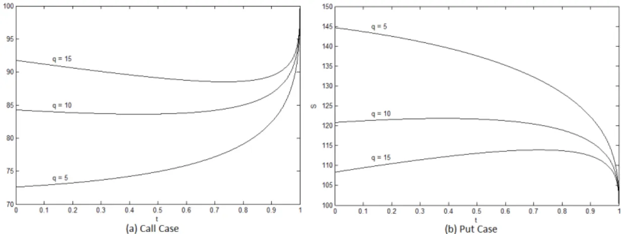
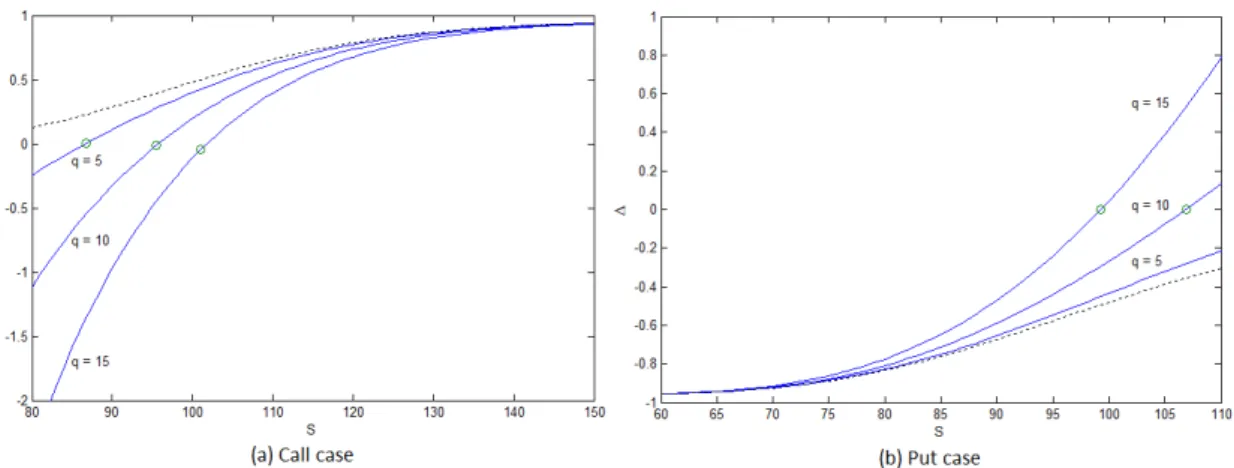
In Figure 5.1 we can see some optimal stopping boundaries and their sensitive to the continuous installment rate q. We first notice that the boundary value is an increasing (decreasing) function of q _{for the call (put) case. This can be easily seen by the}

inequalities *

0

30

Figure 5.1: Stopping boundaries of continuous installment options

(t0,T1,K100, 0.03,r0.02,0.3)

Also, in Figure 5.2 we see the optimal stopping boundaries in dependence of the dividend yield  , from which we can see that now the boundary value is an increasing function of  in both cases.

Figure 5.2: Stopping boundaries of continuous installment options (t0,T1,K100,q10,r0.02,0.2)

Note that in these figures the stopping boundary value at maturity T 1agrees with the strike price K100 as proved in Theorems 4 and 6 in Kimura [21].

31 In Kimura [21] we can see the results from Euler and Gaver-Stehfest method produced by the author, which are a little different than ours. Particularly the results of the Euler method differ significantly from those produced by Gaver-Stehfest algorithm, which caused the author to mistrust the last one. This happened because the author followed two different procedures for each method. For what concerns the Euler method, the author did not apply it to the inversion of the option values *





, ;

c  S q and *





, ;

p  S q . Therefore he used the same procedure than ours. But for the Gaver-Stehfest method, the author applied it directly to the option values, hence getting greater differences between methods.

On Ehrhardt et al. [14] we can also see the results of three of the methods that we are considering, but once again these values are slightly different than ours, perhaps because of a little misleading in their MatLab code.

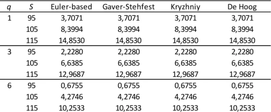
As for our results it can be seen from the tables that all the four methods produce practically equal values, where the absolute difference between the values is less than

5

1 10  .

Table 5.1: Values of continuous installment call options (t0,T1,K100, 0.05,r0.03,0.2)

q S Euler-based Gaver-Stehfest Kryzhniy De Hoog 1 95 3,7071 3,7071 3,7071 3,7071

1 105 8,3994 8,3994 8,3994 8,3994

1 115 14,8530 14,8530 14,8530 14,8530 3 95 2,2280 2,2280 2,2280 2,2280

3 105 6,6385 6,6385 6,6385 6,6385

3 115 12,9687 12,9687 12,9687 12,9687 6 95 0,6755 0,6755 0,6755 0,6755

6 105 4,2746 4,2746 4,2746 4,2746

32

Table 5.2: Values of continuous installment put options (t0,T1,K100, 0.05,r0.03,0.2)

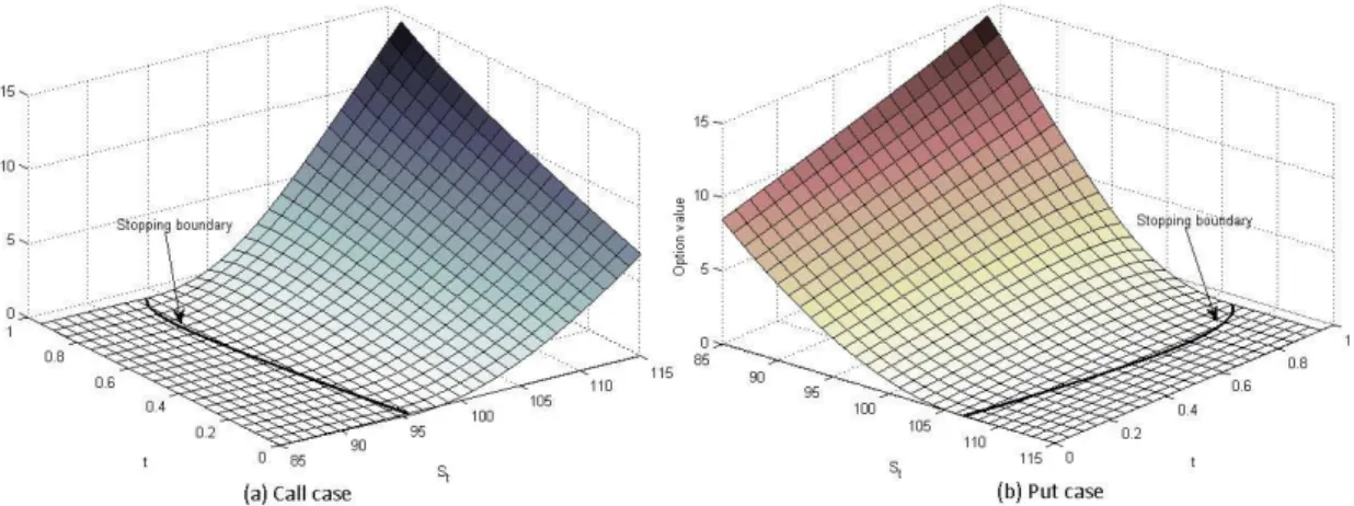
Figure 5.3 presents a 3D plot of the call and the put values in dependence of time t

and the asset priceS_t.

Figure 5.3: The option value for the call and the put (T 1,K 100,0.05,r0.03,0.2,q10)

In order to test the performance of the numerical transform inversion for the LCT of the Greeks, we computed the values of the hedged parameters  (delta),



(gamma) and  _{(theta). Figures 5.4 and 5.5 plot}  and



respectively as functions of S varying the parameterq and Figure 5.6 plots  as a function of S varying the parameter  instead of q. Both figures plot also the associated vanilla options drawn in a dashed line, as well as the stopping boundaries represented by markers. Unlike the conclusions of Kimura who found that the Gaver-Stehfest method performed very poorly if the position is out-of-the-money, we concluded that both methods behave well in the whole region where the stopping boundary is not reached.

q S Euler-based Gaver-Stehfest Kryzhniy De Hoog 1 85 16,9438 16,9438 16,9438 16,9438

1 95 10,3046 10,3046 10,3046 10,3046

1 105 5,5703 5,5703 5,5703 5,5703 3 85 15,0005 15,0005 15,0005 15,0005

3 95 8,4283 8,4283 8,4283 8,4283

3 105 3,8486 3,8486 3,8486 3,8486 6 85 12,1253 12,1253 12,1253 12,1253

6 95 5,7647 5,7647 5,7647 5,7647

33

Figure 5.4: The greek  value for the call and the put case in dependence of q

(t  0,T1,K100, 0.04,r0.02,0.2)

Figure 5.5: The greek  value for the call and the put case in dependence of q

(t  0,T1,K100, 0.04,r0.02,0.2)

Figure 5.6: The greek  value for the call and the put case in dependence of 

34 At this point and looking at Tables 5.1 and 5.2 we still do not have useful information to compare the efficiency of the used methods. The first thing that might be interesting to do is to measure the performance of each method when computing the value of one installment option. In Table 5.3 we can find these results.

Table 5.3: The average of the time it takes to compute the value of one installment option per method.

As we can see the De Hoog method seems to be the best candidate to valuate these options numerically so far.

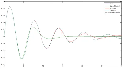
Another way to compare algorithms used for the inverse Laplace transform was proposed by Kryzhniy [23]. The method is based on inverting the function F( ) et whose analytical inverse transform is the delta function on x t . The idea is that finding a method that uses more “focusing” approximation to the delta function is an evident way for improving the provided results. If the algorithm gives us a good approximation of the delta function while inverting etand preserves its peakness while increasing t, it will give good approximations of other functions too.

Figure 5.7 presents the results of reconstructing the delta function by each method. Euler-based Gaver-Stehfest Kryzhniy De Hoog

35

Figure 5.7: The reconstruction of the delta function by the various algorithms.

As we can see, both Euler-summation and De Hoog algorithms give much better results while showing the peaked values. But we cannot ignore the fast oscillations of the curves obtained by both methods, especially by the Euler-summation algorithm.

36 Euler-summation or the De Hoog algorithms, which values are matching with the exact solution.

Figure 5.8: The reconstruction of the damped oscillating function by each method.