Mineração de dados em grande conjuntos de dados complexos

(1)

Data mining in large sets of complex data

(2)

Data mining in large sets of complex data

1

Robson Leonardo Ferreira Cordeiro

Advisor: Prof. Dr. Caetano Traina Jr.

Co-advisor: Prof. Dr. Christos Faloutsos

Doctoral dissertation submitted to the Instituto de Ciências Matemáticas e de Computação - ICMC-USP, in partial fulfillment of the requirements for the degree of the Doctorate Program in Computer Science and Computational Mathematics. REVISED COPY.

USP – São Carlos October 2011

1

This work has been supported by FAPESP (Process Number 2007/01639-4), CNPq and CAPES.

SERVIÇO DE PÓS-GRADUAÇÃO DO ICMC-USP

Data de Depósito: 27/10/2011

(3)

Ficha Catalográfica elaborada pela Seção de Tratamento da Informação da Biblioteca Prof. Achille Bassi- Instituto de Ciências Matemáticas e de Computação – ICMC/USP.

Cordeiro, Robson Leonardo Ferreira

C794d Data mining in large sets of complex data / Robson Leonardo Ferreira Cordeiro. São Carlos, 2011.

135 p.

Tese (Doutorado – Programa de Pós-Graduação em Ciências de Computação e Matemática Computacional). - - Instituto de Ciências Matemática e de Computação,

Universidade de São Paulo, 2011. Orientador: Caetano Traina Jr.

Co-orientador: Christos Faloutsos 1. Correlation Clustering. 2. Moderate-to-high

(4)

Abstract

Due to the increasing amount and complexity of the data stored in the enterprises’ databases, the task of knowledge discovery is nowadays vital to support strategic decisions. However, the mining techniques used in the process usually have high computational costs that come from the need to explore several alternative solutions, in different combinations, to obtain the desired knowledge. The most common mining tasks include data classification, labeling and clustering, outlier detection and missing data prediction. Traditionally, the data are represented by numerical or categorical attributes in a table that describes one element in each tuple. Although the same tasks applied to traditional data are also necessary for more complex data, such as images, graphs, audio and long texts, the complexity and the computational costs associated to handling large amounts of these complex data increase considerably, making most of the existing techniques impractical. Therefore, especial data mining techniques for this kind of data need to be developed. This Ph.D. work focuses on the development of new data mining techniques for large sets of complex data, especially for the task of clustering, tightly associated to other data mining tasks that are performed together. Specifically, this Doctoral dissertation presents three novel, fast and scalable data mining algorithms well-suited to analyze large sets of complex data: the method Halite for correlation clustering; the method

BoW for clustering Terabyte-scale datasets; and the method QMAS for labeling and summarization. Our algorithms were evaluated on real, very large datasets with up to

billions of complex elements, and they always presented highly accurate results, being at least one order of magnitude faster than the fastest related works in almost all cases. The real data used come from the following applications: automatic breast cancer diagnosis, satellite imagery analysis, and graph mining on a large web graph crawled by Yahoo! and also on the graph with all users and their connections from the Twitter social network. Such results indicate that our algorithms allow the development of real time applications

that, potentially, could not be developed without this Ph.D. work, like a software to aid on the fly the diagnosis process in a worldwide Healthcare Information System, or a system to look for deforestation within the Amazon Rainforest in real time.

(5)

(6)

Resumo

O crescimento em quantidade e complexidade dos dados armazenados nas organiza¸cões torna a extra¸cão de conhecimento utilizando técnicas de minera¸cão uma tarefa ao mesmo tempo fundamental para aproveitar bem esses dados na tomada de decisões estratégicas e de alto custo computacional. O custo vem da necessidade de se explorar uma grande quantidade de casos de estudo, em diferentes combina¸cões, para se obter o conhecimento desejado. Tradicionalmente, os dados a explorar são representados como atributos numéricos ou categóricos em uma tabela, que descreve em cada tupla um caso de teste do conjunto sob análise. Embora as mesmas tarefas desenvolvidas para dados tradicionais sejam também necessárias para dados mais complexos, como imagens, grafos, áudio e textos longos, a complexidade das análises e o custo computacional envolvidos aumentam significativamente, inviabilizando a maioria das técnicas de análise atuais quando aplicadas a grandes quantidades desses dados complexos. Assim, técnicas de minera¸cão especiais devem ser desenvolvidas. Este Trabalho de Doutorado visa a cria¸cão de novas técnicas de minera¸cão para grandes bases de dados complexos. Especificamente, foram desenvolvidas duas novas técnicas de agrupamento e uma nova técnica de rotula¸cão e sumariza¸cão que são rápidas, escaláveis e bem adequadas à análise de grandes bases de dados complexos. As técnicas propostas foram avaliadas para a análise de bases de dados reais, em escala de Terabytes de dados, contendo até bilhões de objetos complexos, e elas sempre apresentaram resultados de alta qualidade, sendo em quase todos os casos pelo menos uma ordem de magnitude mais rápidas do que os trabalhos relacionados mais eficientes. Os dados reais utilizados vêm das seguintes aplica¸cões: diagnóstico automático de câncer de mama, análise de imagens de satélites, e minera¸cão de grafos aplicada a um grande grafo da web coletado pelo Yahoo! e também a um grafo com todos os usuários da rede social Twitter e suas conexões. Tais resultados indicam que nossos algoritmos permitem a cria¸cão de aplica¸cões em tempo real que, potencialmente, não poderiam ser desenvolvidas sem a existência deste Trabalho de Doutorado, como por exemplo, um sistema em escala global para o aux´ılio ao diagnóstico médico em tempo real, ou um sistema para a busca por áreas de desmatamento na Floresta Amazônica em tempo real.

T´ıtulo: Minera¸c˜ao de Dados em Grandes Conjuntos de Dados Complexos

Tese apresentada ao Instituto de Ciências Matemáticas e de Computa¸cão - ICMC-USP, como parte dos requisitos para obten¸cão do t´ıtulo de Doutor em Ciências - Ciências de Computa¸cão e Matemática Computacional. VERS ÃO REVISADA.

(7)

(8)

List of Figures

2.1 x-y and x-z projections of four 3-dimensional datasets over axes {x, y, z}. . 13

3.1 Examples of 1-dimensional dense units and clusters existing in a toy database over the dimensions A={x, y}. . . 22 3.2 Examples of p-signaturesin a database over the dimensions A ={x, y}. . . 25 3.3 Examples of global and local orientation in a toy 2-dimensional database. . 29

4.1 Example of an isometric crystal system commonly found in the nature – one specimen of the mineral Halite that was naturally crystallized. . . 36 4.2 x-y and x-z projections of four 3-dimensional datasets over axes {x, y, z}. . 38 4.3 Examples of Laplacian Masks, 2-dimensional hyper-grid cells and the

cor-responding Counting-tree. . . 42 4.4 A mask applied to 1-dimensional data and the intuition on the success of

the used masks. . . 44 4.5 The Counting-tree by tables of key/value pairs in main memory and/or disk. 51 4.6 Illustration of our soft clustering method Halites. . . 52 4.7 Comparison of hard clustering approaches – Halitewas in average at least

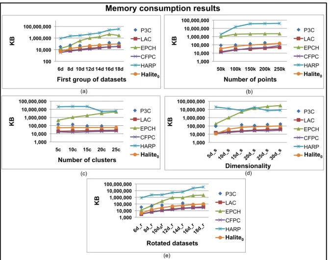
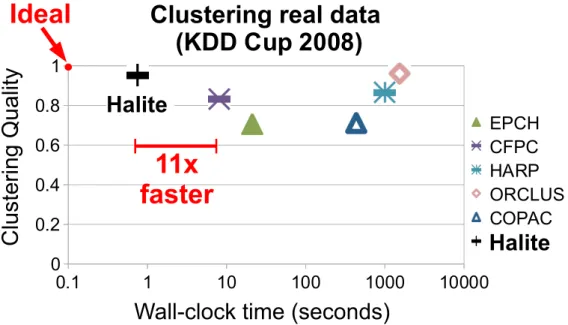
12 times faster than 7 top related works, always giving high quality clusters. 61 4.8 Results on memory consumption for synthetic data. . . 62 4.9 Subspace Quality for synthetic data. . . 62 4.10 Quality versus run time in linear-log scale over 25-dimensional data for

breast cancer diagnosis (KDD Cup 2008). . . 64 4.11 Scalability of Halite and Halites on synthetic data of varying sizes and

dimensionality. . . 65 4.12 Sensitivity analysis. It led to the definition of our default configuration

α= 1E−10 andH = 4. . . 65 4.13 Comparing Halite and Halites with STATPC on data with cluster overlap

(best viewed in color). . . 66 4.14 Ground truth number of clusters versus the number ofβ-clusters found by

Halite over synthetic data. . . 68

5.1 Parallel run overview for ParC (left) and SnI (right - with sampling). . . . 75 5.2 Overview of the Multi-phase Sample-and-Ignore (SnI) Method. . . 78 5.3 Clustering examples for the three data partitioning approaches. . . 83 5.4 Merging and Stitching for the Location-based data partitioning approach. . 85 5.5 Quality versus run time for ParC using distinct data partitioning

ap-proaches (File-based, Random-based and Location-based). . . 89 5.6 Quality versus number r of reducers for ParC, SnI and BoW. . . 90 5.7 Scale-up results regarding the number of reducers r. Our method exhibits

the expected behavior: it starts with near-linear scale-up, and then flattens. 91

(13)

of 10 runs) versus data size for random samples of the YahooEigdataset. 91 5.9 Results provided by BoW for real data from Twitter. Wall-clock time

versus number of reducers in log-log scale. . . 92 5.10 BoW’s results on theTwitterEigand on theSynthetic100 million datasets.

Time (average of 10 runs) versus number of reducers in log-log scale. . . . 93

6.1 One example satellite image of Annapolis (USA), divided into 1,024 (32x32) tiles, only 4 of which are labeled with keywords (best viewed in color). . . . 96 6.2 Examples of representatives spotted in synthetic data. . . 100 6.3 Top-10 outliers for the example dataset in Figure 6.2a, considering the

QMAS representatives from Figure 6.2c (top). . . 101 6.4 The Knowledge Graph G for a toy dataset. . . 103 6.5 Our solution to Problem 1 – low-labor labeling and to Problem 2 – mining

and attention routing on an example satellite image (best viewed in color). 106 6.6 Time versus number of tiles for random samples of the SAT1.5GB dataset. 107 6.7 Comparison of the tested approaches using box plots – quality versus size

of the pre-labeled data. . . 108 6.8 Clustering results provided byQMAS for theGeoEyedataset (best viewed

in color). . . 109 6.9 NR = 6 representatives found by QMAS for the GeoEye dataset, colored

after their clusters (best viewed in color). . . 110 6.10 Top-3 outliers found by QMAS for the GeoEye dataset based on the 6

representatives of Figure 6.9 (best viewed in color). . . 111 6.11 Example with water: labeled data and the corresponding results of a query

for “Water” tiles (best viewed in color). . . 111 6.12 Example with houses: labeled data and the corresponding results of a query

for “House” tiles (best viewed in color). . . 112 6.13 Example with trees: labeled data and the corresponding results of a query

for “Trees” tiles (best viewed in color). . . 112 6.14 Example with docks: labeled data and the corresponding results of a query

for “Dock” tiles (best viewed in color). . . 112 6.15 Example with boats: labeled data and the corresponding results of a query

for “Boat” tiles (best viewed in color). . . 113 6.16 Example with roads: labeled data and the corresponding results of a query

for “Roads” tiles (best viewed in color). . . 113 6.17 Example with buildings: labeled data and the corresponding results of a

query for “Buildings” tiles (best viewed in color). . . 113

(14)

List of Tables

3.1 Properties of clustering algorithms well-suited to analyze moderate-to-high

dimensionality data. . . 32

5.1 Environmental parameters. . . 79

5.2 Other parameters. . . 79

5.3 Summary of datasets. TB: Terabytes; GB: Gigabytes. . . 87

5.4 Environmental parameters for M45. . . 88

6.1 Summary of datasets. MB: Megabytes; GB: Gigabytes. . . 104

7.1 Properties of methods aimed at clustering moderate-to-high dimensionality data, including our methods Halite and BoW. . . 118

(15)

(16)

List of Abbreviations and Acronyms

Halite Method Halite for Correlation Clustering

BoW The Best of both Worlds Method

QMAS Method forQuerying, Mining And Summarizing

Multi-dimensional Databases

KDD Knowledge Discovery in Databases

DB Database

HDFS Hadoop Distributed File System

RWR Random Walk with Restart

MDL Minimum Description Length

SDSS Sloan Digital Sky Survey

API Application Programming Interface

I/O Input / Output

MBR Minimum Bounding Rectangle

MAM Metric Access Methods

CPU Central Processing Unit

PB Petabyte(s)

TB Terabyte(s)

GB Gigabyte(s)

MB Megabyte(s)

RAM Random-Access Memory

GHz Gigahertz

GBdI Databases and Images Group

USP University of S˜ao Paulo

CMU Carnegie Mellon University

(17)

(18)

List of Symbols

d_S _A _d_{-dimensional space.}

S A set of d-dimensional points.S ⊂dS d_S _{- A full} _d_{-dimensional dataset.}

δ

γSk - Points of cluster δγCk. δγSk⊆dS

E A set of axes.

E - Full set of axes for d_S_.

E ={e1, e2. . . ed}, |E|=d

γEk - Axes relevant to a clusterδγCk.

γEk ⊆E, |γEk|=δ

d Dimensionality of dataset d_S_.

η Number of points in dataset d_S_. _η₌ dS

si A point of dataset dS. si ∈dS

sij Value in axis ej of point si. sij ∈[0,1)

δ

γCk A correlation cluster. δγCk =

γEk,δγSk

δ Dimensionality of δ γCk.

k Number of clusters in dataset dS.

γk - Number of correlation clusters.

k - Number of clusters regardless of their types.

T A Counting-tree.

H Number of resolutions in T

h Each level of T.

ξh Side size of cells at level h in T.

ah A cell at level h in T.

α Significance level for the statistical test.

r Number of reducers for parallel run.

m Number of mappers for parallel run.

(19)

Ds Disk speed, i.e. disk transfer rate in bytes per second.

Ns Network speed, i.e. network transfer rate in bytes per second.

Dr Dispersion ratio.

Rr Reduction ratio.

Sr Sampling ratio.

start up cost(t) Start-up cost for t MapReduce tasks.

plug in cost(s) Serial clustering cost regarding the data size s.

I An input collection of complex objects.

Ii One object from I. Ii ∈I

NI The number of objects in I. NI =|I|

L A collection of known labels.

Ll One label from L. Ll ∈L

NL The number of labels in L. NL=|L|

NR The desired number of representatives.

NO The desired number of top outliers.

G The Knowledge Graph. G= (V, X)

V The set of vertexes in G.

X The set of edges in G.

V(Ii) Vertex that represents object Ii in G.

V(Ll) Vertex that represents label Ll in G.

c The restart probability for the random walk.

(20)

Chapter

1

Introduction

This chapter presents an overview of this Doctoral dissertation. It contains brief descriptions of the facts that motivated the work, the problem definition, our main objectives and the central contributions of this Ph.D. work. The following sections describe each one of these topics.

1.1 Motivation

The information generated or collected in digital formats for various application areas is growing not only in the number of objects and attributes, but also in the complexity of the attributes that describe each object [Fayyad, 2007b, Fayyad et al., 1996, Kanth et al., 1998, Korn et al., 2001, Kriegel et al., 2009, Pagel et al., 2000, Sousa, 2006]. This scenario has prompted the development of techniques and tools aimed at, intelligently and automatically, assisting humans to analyze, to understand and to extract knowledge from raw data [Fayyad, 2007b, Fayyad and Uthurusamy, 1996, Sousa, 2006], molding the research area of Knowledge Discovery in Databases – KDD.

The increasing amount of data makes the KDD tasks especially interesting, since they allow the data to be considered as useful resources in the decision-making processes of the organizations that own them, instead of being left unused in disks of computers, stored to never be accessed, such as real ‘tombs of data’ [Fayyad, 2003]. On the other hand, the increasing complexity of the data creates several challenges to the researchers, provided that most of the existing techniques are not appropriate to analyze complex data, such as images, audio, graphs and long texts. Common knowledge discovery tasks are clustering, classification and labeling, identifying measurement errors and outliers, inferring association rules and missing data, and dimensionality reduction.

(21)

1.2 Problem Definition and Main Objectives

The knowledge discovery from data is a complex process that involves high computational costs. The complexity stems from a variety of tasks that can be performed to analyze the data and from the existence of several alternative ways to perform each task. For example, the properties of the various attributes used to describe each data object, such as the fact that they are categorical or continuous, the cardinality of the domains, and the correlations that may exist between different attributes, etc., they all make some techniques more suitable or prevent the use of others. Thus, the analyst must face a wide range of options, leading to a high complexity in the task of choosing appropriate mining strategies to be used for each case.

The high computational cost comes from the need to explore several data elements in different combinations to obtain the desired knowledge. Traditionally, the data to be analyzed are represented as numerical or categorical attributes in a table where each tuple describes an element in the set. The performance of the algorithms that implement the various tasks of data analysis commonly depend on the number of elements in the set, on the number of attributes in the table, and on the different ways in which both tuples and attributes interact with their peers. Most algorithms exhibit super-linear complexity regarding these factors, and thus, the computational cost increases fast with increasing amounts of data.

The discovery of knowledge from complex data, such as images, audio, graphs and long texts, usually includes a preprocessing step, when relevant features are extracted from each object. The features extracted must properly describe and identify each object, since they are actually used in search and comparison operations, instead of the complex object itself. Many features are commonly used to represent each object. The resulting collection of features is named the feature vector.

This Ph.D. work aims at the development of knowledge discovery techniques well-suited to analyze large collections of complex objects described exclusively by their feature vectors, especially for the task of clustering, tightly associated to other data mining tasks that are performed together. Thus, we have explored the following thesis:

Thesis: Although the same tasks commonly performed for traditional data are generally

(22)

1.3 Main Contributions of this Ph.D. Work 3

Therefore, this work is focused on developing techniques well-suited to analyze large collections of complex objects represented exclusively by their feature vectors, automat-ically extracted by preprocessing algorithms. Nevertheless, the proposed techniques can be applied to any kind of complex data, from which sets of numerical attributes of equal dimensionalities can be extracted. Thus, the analysis of multi-dimensional datasets is the scope of our work. The definitions related to this kind of data, which are used throughout this Doctoral dissertation, are presented as follows.

Definition 1 A multi-dimensional dataset dS = {s1, s2, . . . sη} is a set of η points in a d-dimensional space d_S_, d_S _⊂ d_S_{, over the set of axes} _E ₌ _{_e

1, e2, . . . ed}, where d is the dimensionality of the dataset, and η is its cardinality.

Definition 2 A dimension (also called a feature or an attribute)ej ∈ E is an axis of

the space where the dataset is embedded. Every axis related to a dataset must be orthogonal to the other axes.

Definition 3 A point si ∈ dS is a vector si = (si1, si2, . . . sid) that represents a data element in the space d_S_{. Each value} _s

ij ∈ si is a number in R. Thus, the entire dataset is embedded in the d-dimensional hyper-cube Rd_.

1.3 Main Contributions of this Ph.D. Work

With regard to the task of clustering large sets of complex data, an analysis of the literature (see the upcoming Chapter 3) leads us to come to one main conclusion. In spite of the several qualities found in the existing works, to the best of our knowledge, there is no method published in the literature, and well-suited to look for clusters in sets of complex objects, that has any of the following desirable properties: (i)

linear or quasi-linear complexity – to scale linearly or quasi-linearly in terms of

memory requirement and execution time with regard to increasing numbers of points and axes, and; (ii) Terabyte-scale data analysis – to be able to handle datasets of Terabyte-scale in feasible time. On the other hand, examples of applications with Terabytes of high-dimensionality data abound: weather monitoring systems and climate change models, where we want to record wind speed, temperature, rain, humidity, pollutants, etc; social networks like Facebook TM, with millions of nodes, and several attributes per node (gender, age, number of friends, etc); astrophysics data, such as the SDSS (Sloan Digital Sky Survey), with billions of galaxies and attributes like red-shift, diameter, spectrum, etc. Therefore, the development of novel algorithms aimed at overcoming these two aforementioned limitations is nowadays extremely desirable.

(23)

1. The Method Halite for Correlation Clustering: the algorithmHaliteis a fast and scalable density-based clustering algorithm for multi-dimensional data able to analyze large collections of complex data elements. It creates a multi-dimensional grid all over the data space and counts the number of points lying at each hyper-cubic cell provided by the grid. A hyper-quad-tree-like structure, called the Counting-tree, is used to store the counts. The tree is thereafter submitted to a filtering process able to identify regions that are, in a statistical sense, denser than its neighboring regions regarding at least one dimension, which leads to the final clustering result. The algorithm is fast and it has linear or quasi-linear time and space complexity regarding both the data size and the dimensionality. Therefore, Halite tackles the problem of linear or quasi-linear complexity.

2. The Method BoW for Clustering Terabyte-scale Datasets: the method

BoW focuses on the problem of finding clusters in Terabytes of moderate-to-high dimensionality data, such as features extracted from billions of complex data elements. In these cases, a serial processing strategy is usually impractical. Just to read a single Terabyte of data (at 5GB/min on a single modern eSATA disk) one takes more than 3 hours. BoW explores parallelism and can treat as plug-in almost any of the serial clustering methods, including our own algorithm Halite. The major research challenges addressed are (a) how to minimize the I/O cost, taking care of the already existing data partition (e.g., on disks), and (b) how to minimize the network cost among processing nodes. Either of them may become the bottleneck. Our method automatically spots the bottleneck and chooses a good strategy, one of them uses a novel sampling-and-ignore idea to reduce the network traffic. Specifically, BoW combines (a) potentially any serial algorithm used as a plug-in and (b) makes the plug-in run efficiently in parallel, by adaptively balancing the cost for disk accesses and network accesses, which allowsBoWto achieve a very good tradeoff between these two possible bottlenecks. Therefore, BoW tackles the problem of Terabyte-scale data analysis.

3. The Method QMASfor Labeling and Summarization: the algorithmQMAS

(24)

1.4 Conclusions 5

Our algorithms were evaluated on real, very large datasets with up to billions of complex elements, and they always presented highly accurate results, being at least one order of magnitude faster than the fastest related works in almost all cases. The real life data used come from the following applications: automatic breast cancer diagnosis,

satellite imagery analysis, andgraph miningon a large web graph crawled by Yahoo!1 _and

also on the graph with all users and their connections from the Twitter2_{social network. In}

extreme cases, the work presented in this Doctoral dissertation allowed us to spot in only two seconds the clusters present in a large set of satellite images, while the related works took two days to perform the same task, achieving similar accuracy. Such results indicate that our algorithms allow the development of real time applications that, potentially, could not be developed without this Ph.D. work, like a software to aid on the fly the diagnosis process in a worldwide Healthcare Information System, or a system to look for deforestation within the Amazon Rainforest in real time.

1.4 Conclusions

This chapter presented an overview of this Doctoral dissertation with brief descriptions of the facts that motivated the work, the problem definition, our main objectives and the central contributions of this Ph.D. work. The remaining chapters are structured as follows. In Chapter 2, an analysis of the literature is presented, including a description of the main concepts used as a basis for the work. Some of the relevant works found in literature for the task of clustering multi-dimensional data with more than five or so dimensions are described in Chapter 3. Chapters 4, 5 and 6 contain the central part of this Doctoral dissertation. They present the knowledge discovery techniques designed during this Ph.D. work, as well as the experiments performed. Finally, the conclusions and ideas for future work are given in Chapter 7.

1

www.yahoo.com

2

(25)

(26)

Chapter

2

Related Work and Concepts

This chapter presents the main background knowledge related to the doctoral project. The first two sections describe the areas of processing complex data and knowledge discovery in traditional databases. The task of clustering complex databases is discussed in Section 2.3, while the task of labeling such kind of data is described in Section 2.4. Section 2.5 introduces theMapReduceframework, a promising tool for large scale data analysis, which has been proven to offer a valuable support to the execution of data mining algorithms in a parallel processing environment. The last section concludes the chapter.

2.1 Processing Complex Data

Database systems work efficiently with traditional numeric or textual data, but they usually do not provide complete support for complex data, such as images, videos, audio, graphs, long texts, fingerprints, geo-referenced data, among others. However, efficient methods for storing and retrieving complex data are increasingly needed [Mehrotra et al., 1997]. Therefore, many researchers have been working to make database systems more suited to complex data processing and analysis.

The most common strategy is the manipulation of complex data based on features ex-tracted automatically or semi-automatically from the data. This involves the application of techniques that aim at obtaining a set of features (the feature vector) to describe the complex element. Each feature is typically a value or an array of numerical values. The vector resulting from this process should properly describe the complex data, because the mining algorithms rely only on the extracted features to perform their tasks. It is common to find vectors containing hundreds or even thousands of features.

(27)

For example, the extraction of features from images is usually based on the analysis of colors, textures, objects’ shapes and their relationship. Due to its simplicity and low computational cost, the most used color descriptor is the histogram, that counts the numbers of pixels of each color in an image [Long et al., 2002]. The color coherence vector [Pass et al., 1996], the color correlogram [Huang et al., 1997], the metric histogram [Traina et al., 2003] and the cells histogram [Stehling et al., 2003] are other well-known color descriptors. Texture corresponds to the statistical distribution of how the color varies in the neighborhood of each pixel of the image. Texture analysis is not a trivial task and it usually leads to higher computational costs than the color analysis does. Statistical methods [Duda et al., 2001, Rangayyan, 2005] analyze properties, such as granularity, contrast and periodicity to differentiate textures, while syntactic methods [Duda et al., 2001] perform this task by identifying elements in the image and analyzing their spatial arrangements. Co-occurrence matrices [Haralick et al., 1973], Gabor [Daugman, 1985, Rangayyan, 2005] and wavelet transforms [Chan and Shen, 2005] are examples of such methods. The descriptors of shapes commonly have the highest computational costs compared to the other descriptors, and therefore, they are used mainly in specific applications [Pentland et al., 1994]. There are two main techniques to detect shapes: the geometric methods of edge detection [Blicher, 1984, Rangayyan, 2005], which analyze length, curvature and signature of the edges, and the scalar methods for region detection [Sonka et al., 1998], which analyze the area, “eccentricity”, and “rectangularity”.

It is possible to say that, besides the feature extraction process, there are still two main problems to be addressed in order to allow efficient management of complex data. The first is the fact that the extractors usually generate many features (hundreds or even thousands). As described in the upcoming Section 2.2, it impairs the data storage and retrieval techniques due to the “curse of dimensionality” [Beyer et al., 1999, Korn et al., 2001, Kriegel et al., 2009, Moise et al., 2009, Parsons et al., 2004]. Therefore, dimensionality reduction techniques are vital to the success of strategies for indexing, retrieving and analyzing complex data. The second problem stems from the need to compare complex data by similarity, because it usually does not make sense to compare them by equality, as it is commonly done for traditional data [Vieira et al., 2004]. Moreover, the total ordering property does not hold among complex data elements -one can only say that two elements are equal or different, since there is no explicit rule to sort the elements. This fact distinguishes complex data elements even more from the traditional elements. The access methods based on the total ordering property do not support queries involving comparisons by similarity. Therefore, a new class of access methods was created, known as the Metric Access Methods (MAM), aimed at allowing searches by similarity. Examples of such methods are theM-tree[Ciaccia et al., 1997], the

(28)

2.2 Knowledge Discovery in Traditional Data 9

[Vieira et al., 2004], which are considered to be dynamic methods, since they allow data updates without the need to rebuild the structure.

The main principle for these techniques is the representation of the data in a metric space. The similarity between two elements is calculated by a distance function acting as a metric applied to the pair of elements in the same domain. The definitions of a metric space and the main types of queries applied to it are as follows.

Definition 4 A metric space is defined as a pair hS_{, m}_i_{, where} S _{is the data domain}

and m : S_×S _→ R+ _{a distance function acting as a metric. Given any} _s₁_{, s}₂_{, s}₃ _∈ S_,

this function must respect the following properties: (i) symmetry, m(s1, s2) = m(s2, s1);

(ii) non-negativity, 0 < m(s1, s2) < ∞,∀ s1 6= s2; (iii) identity, m(s1, s1) = 0; and (iv)

triangle inequality, m(s1, s2)≤m(s1, s3) +m(s3, s2),∀ s1, s2, s3 ∈S.

Definition 5 A range query in a metric space receives as input an object s1 ∈ S and

one specific range ǫ. It returns all objects si, provided that m(si, s1) ≤ ǫ, based on the

distance function m.

Definition 6 Ak nearest neighbor queryin a metric space receives as input an object

s1 ∈S and an integer value k ≥1. It returns the set of the k objects closest to s1, based

on the distance function m.

One particular type of metric space is the d-dimensional space, for which a distance function is defined, denoted as_d

S_{, m}_{. This case is especially interesting for this Doctoral}

dissertation, since it allows posing similarity queries over complex objects represented by feature vectors of equal cardinality in a multi-dimensional dataset.

2.2 Knowledge Discovery in Traditional Data

(29)

major problem to be minimized is the “curse of dimensionality” [Beyer et al., 1999, Korn et al., 2001, Kriegel et al., 2009, Moise et al., 2009, Parsons et al., 2004], a term referring to the fact that increasing the number of attributes in the objects quickly leads to significant degradation of the performance and accuracy of existing techniques to access, store and process data. This occurs because data represented in high dimensional spaces tend to be extremely sparse and all the distances between any pair of points tend to be very similar, with respect to various distance functions and data distributions [Beyer et al., 1999, Kriegel et al., 2009, Parsons et al., 2004]. Dimensionality reduction is the most common technique applied to minimize this problem. It aims at obtaining a set of relevant and non-correlated attributes that allow representing the data in a space of lower dimensionality with minimum loss of information. The existing approaches are: feature selection, which discards among the original attributes, the ones that contribute with less information to the data objects; and feature extraction, which creates a reduced set of new features, formed by linear combinations of the original attributes, able to represent the data with little loss of information [Dash et al., 1997].

The mining task is a major step in the KDD process. It involves the application of data mining algorithms chosen according to the goal to be achieved. Such tasks are classified as: predictive tasks, which seek a model to predict the value of an attribute based on the values of other attributes, by generalizing known examples, and descriptive tasks, which look for patterns that describe the intrinsic data behavior [Sousa, 2006].

Classification is a major predictive mining task. It considers the existence of a training set with records classified according to the value of an attribute (target attribute or class) and a test set, in which the class of each record is unknown. The main goal is to predict the values of the target attribute (class) in the database records to be classified. The algorithms perform data classification by defining rules to describe correlations between the class attribute and the others. Examples of such algorithms are genetic algorithms [Ando and Iba, 2004, Zhou et al., 2003] and algorithms based on decision trees [Breiman et al., 1984], on neural networks [Duda et al., 2000] or on the Bayes theorem (Bayesian classification) [Zhang, 2004].

Clustering is an important descriptive task. It is defined as: “The process of grouping the data into classes or clusters, so that objects within a cluster have high similarity in comparison to one another but are very dissimilar to objects in other clusters.”

(30)

2.3 Clustering Complex Data 11

are k-Means [Lloyd, 1982, MacQueen, 1967, Steinhaus, 1956], k-Harmonic Means [Zhang et al., 2000], DBSCAN [Ester et al., 1996] and STING [Wang et al., 1997].

The last step in the process of knowledge discovery is the result evaluation. At this stage, the patterns discovered in the previous step are interpreted and evaluated. If the patterns refer to satisfactory results (valid, novel, potentially useful and ultimately understandable), the knowledge is consolidated. Otherwise, the process returns to a previous stage to improve the results.

2.3 Clustering Complex Data

Complex data are usually represented by vectors with hundreds or even thousands of features in a multi-dimensional space, as described in Section 2.1. Each feature represents a dimension of the space. Due to the curse of dimensionality, traditional clustering methods, such as k-Means [Lloyd, 1982, MacQueen, 1967, Steinhaus, 1956], k-Harmonic Means [Zhang et al., 2000], DBSCAN [Ester et al., 1996] and STING [Wang et al., 1997], are commonly inefficient and ineffective for these data [Aggarwal and Yu, 2000, Aggarwal et al., 1999, Agrawal et al., 1998, 2005]. The main factor that leads to their inefficiency is that they often have super-linear computational complexity on both cardinality and dimensionality. Traditional methods are also often ineffective, when applied to high dimensional data, as the data tend to be very sparse in the multi-dimensional space and the distances between any pair of points usually become very similar to each other, regarding several data distributions and distance functions [Beyer et al., 1999, Kriegel et al., 2009, Moise et al., 2009, Parsons et al., 2004]. Thus, traditional methods do not solve the problem of clustering large, complex datasets [Aggarwal and Yu, 2000, Aggarwal et al., 1999, Agrawal et al., 1998, 2005, Domeniconi et al., 2007, Kriegel et al., 2009, Moise et al., 2009, Parsons et al., 2004, Tung et al., 2005].

(31)

step for traditional clustering, they do not solve the problem of clustering large, complex datasets. [Aggarwal and Yu, 2000, Aggarwal et al., 1999, Agrawal et al., 1998, 2005, Domeniconi et al., 2007].

Since high dimensional data often present correlations local to subsets of elements and dimensions, the data are likely to present clusters that only exist in subspaces of the original data space. In other words, although high dimensional data usually do not present clusters in the space formed by all dimensions, the data tend to form clusters when the points are projected into subspaces generated by reduced sets of original dimensions or linear combinations of them. Moreover, different clusters may be formed in distinct subspaces. Several recent studies support this idea and a recent survey on this area is presented at [Kriegel et al., 2009].

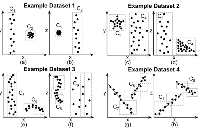
Figure 2.1 exemplifies the existence of clusters in subspaces of four 3-dimensional databases over the axes E = {x, y, z}. Figure 2.1a shows a 3-dimensional dataset projected onto axesxandy, while Figure 2.1b shows the same dataset projected onto axes

x and z. There exist two clusters in this data, C1 and C2. None of the clusters present

a high density of points in the 3-dimensional space, but each cluster is a dense, elliptical object in one subspace. Thus, the clusters exist in subspaces only. ClusterC1 exists in the

subspace formed by axes x and z, while cluster C2 exists in the subspace{x, y}. Besides

elliptical clusters, real data may have clusters that assume any shape in their respective subspaces. The clusters must only be dense in that subspace. To illustrate this fact, we present ‘star-shaped’ and ‘triangle-shaped’ clusters in another dataset (Figure 2.1c: x-y

projection; Figure 2.1d: x-zprojection) and ‘curved’ clusters in one third example dataset (Figure 2.1e: x-y projection; Figure 2.1f: x-z projection).

Such clusters may also exist in subspaces formed by linear combinations of original axes. That is, clusters like the ones in our previous examples may be arbitrarily rotated

in the space, thus not being aligned to the original axes. For example, Figures 2.1g and 2.1h respectively plot x-yand x-z projections of one last 3-dimensional example dataset. Similarly to clustersC1 andC2, the clusters in this data are also dense, elliptical objects in

(32)

2.3 Clustering Complex Data 13 x y C₁ (a) C₂ x z (b) C₁ C2

Example Dataset 1

x y (e) x z (f) C₅ C₆ C₅ C6

Example Dataset 3

x z (d) x y (c) C₃

C₄ C3

C₄

Example Dataset 2

x z (h) C7 C₈ x y (g) C₇ C₈

Example Dataset 4

Figure 2.1: x-y and x-z projections of four 3-dimensional datasets over axes {x, y, z}. From (a) to (f): clusters in the subspaces {x, y} and {x, z}. (g) and (h): clusters in subspaces formed by linear combinations of {x, y, z}.

be identified without knowing the respective subsets. In other words, clustering complex data is not possible due to the high dimensionality, but the dimensionality reduction is incomplete without the prior knowledge of the data clusters where local correlations occur. The most common strategy used to untangle this knotty problem is to unify both tasks, clustering and dimensionality reduction, creating a single task. Several methods have used this idea in order to look for clusters together with the subspaces where the clusters exist. According to a recent survey [Kriegel et al., 2009], such methods differ from each other in two major aspects: (i) the search strategy used in the process, which can be top-down orbottom-up, and (ii) the characteristics of the clusters sought.

The Bottom-up algorithms usually rely on a property named downward closure or

(33)

cluster will stand out, i.e. at least one space region will be dense enough, when the data are projected into any subspace formed by the original dimensions.

Based on a clustering characterization criterion in which the downward closure

property applies, bottom-up algorithms assume that: if a cluster exists in a space of high dimensionality, it has to exist or to be part of some cluster in all subspaces of lower dimensionality formed by original dimensions [Agrawal et al., 2005, Kriegel et al., 2009, Parsons et al., 2004]. These methods start analyzing low dimensional subspaces, usually 1-dimensional ones, in order to identify the subspaces that contain clusters. The subspaces selected are then united in a recursive procedure that allows the identification of subspaces of higher dimensionality in which clusters also exist. Various techniques are used to spot and to prune subspaces without clusters so that they are ignored in the process, minimizing the computational cost involved, but, in general, the main shortcomings of

bottom-upmethods are: (i) they often have super-linear computational complexity or even exponential complexity regarding the dimensionality of the subspaces analyzed, and (ii) fixed density thresholds are commonly used, assuming that clusters in high dimensional spaces are as dense as clusters in subspaces of smaller dimensionality, which is unlikely to be true in several cases.

The Top-down algorithms assume that the analysis of the space with all dimensions can identify patterns that lead to the discovery of clusters existing in lower dimensional subspaces only [Parsons et al., 2004]. This assumption is known in literature as thelocality assumption [Kriegel et al., 2009]. After identifying a pattern, the distribution of points surrounding the pattern in the space with all dimensions is analyzed to define whether or not the pattern refers to a cluster and the subspace in which the possible cluster is better characterized. The main drawbacks oftop-downalgorithms are: (i) they often have super-linear computational complexity, though not exponential complexity, with regard to the data dimensionality, and; (ii) there is no guarantee that the analysis of the data distribution in the space with all dimensions is always sufficient to identify clusters that exist in subspaces only.

Clustering algorithms for high dimensional data also differ from each other in the characteristics of the clusters that they look for. Some algorithms look for clusters that form a dataset partition, together with a set of outliers, while other algorithms partition the database regarding specific subspaces, so that the same data element can be part of two or more clusters that overlap with each other in the space with all dimensions, as long as the clusters are formed in different subspaces [Parsons et al., 2004]. Finally, the subspaces analyzed by these methods may be limited to subsets of the original dimensions or may not be limited to them, thus including subspaces formed by linear combinations of the original dimensions [Kriegel et al., 2009].

Subspace clustering algorithms aim at analyzing projections of the dataset into

(34)

2.4 Labeling Complex Data 15

corresponding data projection, these algorithms operate similarly to traditional clustering algorithms, partitioning the data into disjoint sets of elements, namedsubspace clusters, and a set of outliers. A data point can belong to more than one subspace cluster, as long as the clusters exist in different subspaces. Therefore, subspace clusters arenot necessarily disjoint. Examples of subspace clustering algorithms are: CLIQUE [Agrawal et al., 1998, 2005], ENCLUS [Cheng et al., 1999], SUBCLU [Kailing et al., 2004], FIRES [Kriegel et al., 2005], P3C [Moise et al., 2006, 2008] and STATPC [Moise and Sander, 2008].

Projected clustering algorithms aim at partitioning the dataset intodisjoint sets

of elements, named projected clusters, and a set of outliers. A subspace formed by the original dimensions is assigned to each cluster, and the cluster elements are densely grouped, when projected into the respective subspace. Examples of projected clustering algorithms in literature are: PROCLUS [Aggarwal et al., 1999], DOC/FASTDOC [Procopiuc et al., 2002], PreDeCon [Bohm et al., 2004], COSA [Friedman and Meulman, 2004], FINDIT [Woo et al., 2004], HARP [Yip and Ng, 2004], EPCH [Ng and Fu, 2002, Ng et al., 2005], SSPC [Yip et al., 2005], P3C [Moise et al., 2006, 2008] and LAC [Al-Razgan and Domeniconi, 2006, Domeniconi et al., 2004, 2007].

Correlation clustering algorithms aim at partitioning the database in a manner

analogous to what occurs with projected clustering techniques - to identifydisjointclusters and a set of outliers. However, the clusters identified by such methods, namedcorrelation clusters, are composed of densely grouped elements in subspaces formed by the original dimensions of the database, or by their linear combinations. Examples of correlation clustering algorithms found in literature are: ORCLUS [Aggarwal and Yu, 2002, 2000], 4C [Bohm et al., 2004], CURLER [Tung et al., 2005], COPAC [Achtert et al., 2007] and CASH [Achtert et al., 2008]. Notice that, to the best of our knowledge, CURLER is the only method found in literature that spots clusters formed by non-linear, local correlations, besides the ones formed by linear, local-correlations.

2.4 Labeling Complex Data

In this section, we assume that the clustering algorithms aimed at analyzing complex data, such as the ones cited in the previous section, can also serve as a basis to perform one distinct data mining task – the task of labeling large sets of complex objects, as we will discuss in the upcoming Chapter 6. For that reason, the following paragraphs introduce some background knowledge related to the task of labeling complex data, i.e., the task of analyzing a given collection of complex objects, in which a few objects have labels, in order to spot appropriate labels for the remaining majority.

(35)

the database records to be labeled. Unlike other data mining tasks, the task of labeling is not completely defined in the literature and slight conceptual divergences exist in the definitions provided by distinct authors, while some authors consider that labeling is one type of classification or use other names to refer to it (e.g., captioning). In this Ph.D. work, we consider that labeling refers to a generalized version of the classification task, in which the restriction of mandatorily assigning one and only one label to every data object does not exist. Specifically, we assume that labeling generalizes the task of classification with regard to at most three aspects: (i) it may consider that the dataset commonly contains objects that differ too much from the labeled training examples, which should be returned to the user as outliers that potentially deserve a new label of their own; (ii) it may allow any object to receive more than one appropriate label; and (iii) it may use hierarchies of labels, in a way that each object can be assigned to entire paths in the hierarchy, instead of being linked to individual labels only.

Regarding complex data, labeling has been mostly applied to image datasets and also to sets of image regions segmented or arbitrarily extracted from larger images. There is an extensive body of work on the labeling of unlabeled regions extracted from partially labeled images in the computer vision field, such as image segmentation and region classification [Lazebnik and Raginsky, 2009, Shotton et al., 2006, Torralba et al., 2008]. The Conditional Random Fields (CRF) and boosting approach [Shotton et al., 2006] shows a competitive accuracy for multi-label labeling and segmentation, but it is relatively slow and requires many training examples. The KNN classifier [Torralba et al., 2008] may be the fastest way for image region labeling, but it is not robust against outliers. Also, the Empirical Bayes approach [Lazebnik and Raginsky, 2009] proposes to learn contextual information from unlabeled data. However, it may be difficult to learn the context from several types of complex data, such as from satellite images.

The Random Walk with Restart (RWR) [Tong et al., 2008] algorithm has served as a basis to other labeling methods. The idea is to perform labeling by creating a graph to represent the input complex objects to be labeled, the given example labels and the similarities existing between the objects. Then, random walks in this graph allow spotting the most appropriate labels for the remaining unlabeled objects. In general, RWR consists into performing walks in a graph according to the following strategy: a random walker starts a walk from a vertexV of the graph, and, at each time step, the walker either goes back to the initial vertex V, with a user-defined probability c, or it goes to a randomly chosen vertex that shares an edge with the current vertex, with probability 1−c. The intuition is that this procedure provides an appropriate relevance score between two graph nodes, since the steady state probability that a random walker will find itself in a vertex

V′_{, always restarting the walk from a vertex}_V_{, is a way to measure the closeness between}

(36)

2.5 MapReduce 17

GCap [Pan et al., 2004] is one of the most famous labeling methods that uses random walks with restarts as a basis. GCap proposes a graph-based strategy for automatic image labeling, which can also be applied to any set of multimedia objects. It represents images and label keywords by multiple layers of nodes in a graph and captures the similarities between pairs of images by creating edges to link the nodes that refer to similar images. The known labels become links between the respective images and keywords. This procedure creates a tri-partite graph that represents the input images and labels, besides the existing similarities between the images. Given an image node of interest, random walks with restarts (RWR) are used to perform proximity queries in this graph, allowing GCap to automatically find the best annotation keyword for the respective image. Unfortunately, GCap remains rather inefficient, since it searches for the nearest neighbors of every image in the image feature space to create edges between similar image nodes, and this operation is super-linear even with the speed up offered by many approximate nearest-neighbor finding algorithms (e.g., the ANN Library [Mount and Arya]).

2.5 MapReduce

The large amounts of data collected by the enterprises are accumulating data, and today it is already feasible to have Terabyte- or even Petabyte-scale datasets that must be submitted for data mining processes (e.g., Twitter crawl: > 12 TB, Yahoo! operational data: 5 Petabytes [Fayyad, 2007a]), such as the processes of clustering and labeling complex data. However, the use of serial data mining algorithms, like the ones described in the previous sections, to analyze such huge amounts of data is clearly an impractical task. Just to read a single Terabyte of data (at 5GB/min on a single modern eSATA disk) one takes more than 3 hours. Therefore, to improve the existing serial data mining methods in order to make them run efficiently in parallel is nowadays extremely desirable. With that in mind, this section describes the MapReduceframework, a promising tool for large-scale, parallel data analysis, which has been proving to offer a valuable support to the execution of data mining algorithms in a parallel processing environment.

MapReduce is a programming framework [Dean and Ghemawat, 2004] fostered by Google1 _{to process large-scale data in a massively parallel way.} _MapReduce _{has two}

major advantages: the programmer is oblivious of the details related to the data storage, distribution, replication, load balancing, etc.; and furthermore, it adopts the familiar concept of functional programming. The programmer needs to specify only two functions, a map and a reduce. The typical framework is as follows [L¨ammel, 2008]: (a) the map

stage passes over the input file and outputs (key, value) pairs; (b) the shuffling stage transfers the mappers output to the reducers based on the key; (c) the reduce stage processes the received pairs and outputs the final result. Due to its scalability, simplicity

1

(37)

and the low cost to build large clouds of computers, MapReduce is a very promising tool for large scale, parallel data analysis, which has already being reflected in the academia (e.g., [Papadimitriou and Sun, 2008] [Kang et al., 2009] [Kang et al., 2010]).

Hadoopis the open source implementation ofMapReduce. Hadoopprovides the Hadoop Distributed File System (HDFS) [Had], HBase [Wiki], which is a way to efficiently store and handle semi-structured data as Google’s BigTable storage system [Chang et al., 2006], and PIG, a high level language for data analysis [Olston et al., 2008].

2.6 Conclusions

(38)

Chapter

3

Clustering Methods for

Moderate-to-High Dimensionality Data

Traditional clustering methods are usually inefficient and ineffective over data with more than five or so dimensions. In Section 2.3, we discuss the main reasons that lead to this fact. It is also mentioned that the use of dimensionality reduction methods does not solve the problem, since it allows one to treat only the global correlations in the data. Correlations local to subsets of the data cannot be identified without the prior identification of the data clusters where they occur. Thus, algorithms that combine dimensionality reduction and clustering into a single task have been developed to look for clusters together with the subspaces of the original space where they exist. Some of these algorithms are described in this chapter. Specifically, we first present a brief survey on the existing algorithms, and later we detail four of the most relevant ones. Then, in order to help one to evaluate and to compare the algorithms, we conclude the chapter by presenting a table to link some of the most relevant techniques with the main desirable properties that any clustering technique for moderate-to-high dimensionality data should have. The general goal of the chapter is to identify the main strategies already used to deal with the problem, besides the key limitations of the existing techniques.

Remark: the concepts considered by each technique are not equal, in spite of being similar in several cases, and thus, slight conceptual divergences are contemplated by the original notation. To avoid conflicts in the concepts, this chapter describes each algorithm following the original notation used by its authors. Consequently, the list of symbols shown at the beginning of this Doctoral dissertation should be disregarded in this chapter.

(39)

3.1 Brief Survey

CLIQUE [Agrawal et al., 1998, 2005] was probably the first technique aimed at finding clusters in subspaces of multi-dimensional data. It uses a bottom-up approach, dividing 1-dimensional data projections into a user-defined number of partitions and merging dense partitions to spot clusters in subspaces of higher dimensionality. CLIQUE scales exponentially regarding the cluster dimensionality and it relies on a fixed density threshold that assumes high-dimensional clusters to be as dense as low-dimensional ones, an assumption that is often unrealistic. Several posterior works, such as ENCLUS [Cheng et al., 1999], EPCH [Ng et al., 2005], P3C [Moise et al., 2006, 2008], SUBCLU [Kr¨oger et al., 2004] and FIRES [Kriegel et al., 2005] improve the ideas of CLIQUE to reduce its drawbacks, but they are still typically super-linear in space or in running time.

PROCLUS [Aggarwal et al., 1999] proposed a top-down clustering strategy, assuming what is known in the literature as thelocality assumption: the analysis of the space with all dimensions is sufficient to find patterns that lead to clusters that only exist in subspaces. PROCLUS is a k-medoid method that assigns to each medoid a subspace of the original axes. Each point is assigned to the closest medoid in its subspace. An iterative process analyzes the points distribution of each cluster in each axis and the axes in which the cluster is denser form its subspace. PROCLUS scales super-linearly on the number of points and axes and it only finds clusters in subspaces formed by the original axes.

ORCLUS [Aggarwal and Yu, 2002, 2000] and CURLER [Tung et al., 2005] improve the ideas of PROCLUS to find arbitrarily oriented correlation clusters. They analyze each cluster’s orientation, based on the data attributes eigenvector with the biggest eigenvalue, in an iterative process that merges close clusters with similar orientations. CURLER spots even non-linear, local correlations, but it has a quadratic time complexity regarding the number of clusters and their dimensionalities, and its complexity is cubic with respect to the data dimensionality. Other well-known, top-down methods are: DOC/FASTDOC [Procopiuc et al., 2002], PkM [Agarwal and Mustafa, 2004], LAC [Domeniconi et al., 2007], RIC [B¨ohm et al., 2006], LWC/CLWC [Cheng et al., 2008], PreDeCon [Bohm et al., 2004], OCI [B¨ohm et al., 2008], FPC/CFPC [Yiu and Mamoulis, 2005], COSA [Friedman and Meulman, 2004], HARP [Yip et al., 2004] and STATPC [Moise and Sander, 2008].

(40)

3.2 CLIQUE 21

CASH [Achtert et al., 2008] uses a novel idea that does not rely on the locality assumption. Based on the Hough transform [Hough, 1962], it proposes to map the data space into a parameter space defining the set of all possible arbitrarily oriented subspaces. Then, it analyzes the parameter space to find those among all the possible subspaces that accommodate many database objects, leading to the identification of correlation clusters. Unfortunately, CASH remains rather inefficient, as it has a cubic average time complexity regarding the data dimensionality d and its worst case time complexity is O 2d

.

CARE [Zhang et al., 2008] formalizes the correlation clustering problem as the problem of finding feature subsets strongly correlated with regard to large portions of the input dataset. It uses the Spectrum Theory to study the monotonicity properties of the problem, which allows the proposal of heuristics to prune the problem’s search space. However, CARE has four user-defined input parameters and it usually scales quadratically on the data dimensionality, with an exponential, theoretical worst case time complexity.

This section presented a brief survey on the existing algorithms well-suited to analyze moderate-to-high dimensionality data. A recent survey on this area is given by [Kriegel et al., 2009]. In the next sections, four of the most relevant algorithms are detailed.

3.2 CLIQUE

The method CLIQUE [Agrawal et al., 1998, 2005] was probably the first method aimed at finding clusters in subspaces of multi-dimensional data. It proposes abottom-upsearch strategy, to identify subspace clusters.

The process starts by analyzing the input data projected into the 1-dimensional subspaces formed by each of the original dimensions. In this step, a data scan is performed to partition each projection into ξ equal sized intervals, which enables the creation of histograms that represent the points distribution regarding each interval and dimension. An interval is considered to be adense unitwhen the percentage of elements inside it, with regard to the total number of elements, is greater than or equal to a density threshold τ. The values of ξ and τ are user-defined input parameters.

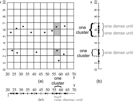
Examples of dense units are illustrated in Figure 3.1, which was adapted from [Agrawal et al., 2005]. Figures 3.1a, 3.1b and 3.1c respectively present an example dataset over the set of dimensionsA={x, y}and its projections in the 1-dimensional subspaces formed by dimensionsxand y. The database contains a total of 14 elements and each 1-dimensional projection is partitioned into ξ = 10 equal sized intervals. Given a density threshold

(41)

y

x x

(a) (b)

y

(c)

one dense unit

}

one dense unit

}

one dense unit

}

one dense unit

}

one cluster

{

one cluster

{

one cluster

{

Figure 3.1: Examples of 1-dimensional dense units and clusters existing in a toy

database over the dimensions A = {x, y}. The figure was adapted from [Agrawal et al., 2005].

Once the 1-dimensional dense units are identified, the process continues in order to find k-dimensional dense units, for k >1. A pair of dense units in subspaces with k−1 dimensions generates a candidate k-dimensional dense unit if and only if the respective subspaces share exactlyk−2 dimensions and both units are in the same positions regarding the shared dimensions. After identifying all candidate k-dimensional dense units, a data scan allows the algorithm to verify if the candidates are actually dense units. A candidate is said to be a dense unit if the number of points that fall into it is enough with regard to the threshold τ. The process continues recursively and it ends when, in an iteration: new dense units are not found, or; the space with all dimensions is analyzed.

In our running example from Figure 3.1, the 1-dimensional dense units identified lead to the existence of three candidates, 2-dimensional dense units, filled in gray in Figure 3.1a. These are described as (2 ≤ x < 3)∧(55 ≤ y < 60), (5 ≤x < 6)∧(55 ≤ y <60) and (6≤x <7)∧(55≤y <60). However, after a data scan, it is possible to notice that none of the candidates has three or more points, which is the minimum number of points needed to spot a dense unit in this example. Thus, the recursive process is terminated.

(42)

3.3 P3C 23

Thus, CLIQUE considers that, if needed, it is better to prune the subspace formed by dimension y than the one formed by x.

Pruning is performed as follows: at each iteration of the process, the dense units found are grouped according to their respective subspaces. The subspaces are then put into a list, sorted in descending order regarding the sum of points in their dense units. The principle Minimum Description Length (MDL) [Grunwald et al., 2005, Rissanen, 1989] is then used to partition this list, creating two sublists: interesting subspaces and

uninteresting subspaces. The MDL principle allows maximizing the homogeneity of the values in the sublists regarding the sum of points in the dense units of each subspace. After this step is finished, the dense units that belong to the uninteresting subspaces are discarded and the recursive process continues, considering only the remaining dense units. Once the recursive process is completed, the dense units identified are merged so that maximum sets of dense units adjacent in one subspace indicate clusters in that subspace. The problem of finding maximum sets of adjacent, dense units is equivalent to a well-known problem in the Graph Theory, the search for connected subgraphs. This is verified considering a graph whose vertices correspond to dense units in one subspace and edges connect two vertices related to adjacent, dense units, i.e., the ones that have a common face in the respective subspace. Thus, a depth-first search algorithm [Aho et al., 1974] is applied to find the maximum sets of adjacent, dense units defining the clusters and their corresponding subspaces. In our example, the dense units found in Figure 3.1b form two clusters in the subspace defined by dimension x. One cluster is related to the dense unit (2≤x <3) while the other refers to the pair of adjacent dense units (5≤x <6) and (6 ≤ x < 7). Finally, the subspace of dimension y contains a single cluster, represented by the dense unit (55≤y <60), and no cluster exists in the 2-dimensional space.

The main shortcomings of CLIQUE are: (i) even considering the pruning of subspaces proposed, the time complexity of the algorithm is still exponential with regard to the dimensionality of the clusters found; (ii) due to the pruning technique used, there is no guarantee that all clusters will be found; (iii) there is no policy suggested to define appropriate values to the parameters ξ and τ, and; (iv) the density parameter τ assumes that clusters in subspaces of high dimensionality should be as dense as clusters in subspaces of lower dimensionality, a fact which is often unrealistic.

3.3 P3C

P3C [Moise et al., 2006, 2008] is a well-known method for clustering moderate-to-high dimensional data. It uses abottom-upsearch strategy that allows findingsubspace clusters

Mineração de dados em grande conjuntos de dados complexos

Data mining in large sets of complex data

Data mining in large sets of complex data

Robson Leonardo Ferreira Cordeiro

Abstract

Resumo

Contents

List of Figures

List of Tables

List of Abbreviations and Acronyms

List of Symbols

Chapter

1

Introduction

1.1

Motivation

1.2

Problem Definition and Main Objectives

1.3

Main Contributions of this Ph.D. Work

1.4

Conclusions

Chapter

2

Related Work and Concepts

2.1

Processing Complex Data

2.2

Knowledge Discovery in Traditional Data

2.3

Clustering Complex Data

Example Dataset 1

Example Dataset 3

Example Dataset 2

Example Dataset 4

2.4

Labeling Complex Data

2.5

MapReduce

2.6

Conclusions

Chapter

3

Clustering Methods for

Moderate-to-High Dimensionality Data

3.1

Brief Survey

3.2

CLIQUE

}

}

}

}

{

{

{

3.3

P3C