Properties Based Simplification of 2D Urban Area Map Object
Jagdish Lal Raheja and Umesh Kumar
Central Electronics Engineering Research Institute (CEERI)/ Council of Scientific and Industrial Research (CSIR), Pilani-Rajasthan, 333031, India
Abstract
For a long time, Geo-spatial information was printed on paper maps whose contents were produced once for specific purposes and scales. These maps are characterized by their portability, good graphic quality, high image resolution and good placement of their symbols and labels. These maps have been generated manually by cartographers whose work was hard and fastidious. Today, Computers are in use to generate the map as per requirement called the cartographic generalization. The purpose of cartographic generalization is to represent a particular situation adapted to the needs of its users, with adequate legibility of the real situation and its perceptional congruity with the representation. Interesting are those situations which, to some degree, vary from the real situation in nature. In this paper, a simple approach is presented for the simplification of contour, roads and building ground plans that are represented as 2D line, square and polygon segments. As it is important to preserve the overall characteristics of the buildings; the lines are geometrically simplified with regard to geometric relations. It also holds true for contour and road data. In this paper, an appropriate transformation and visualization of contour and building data is presented.
Keywords: Cartographic Generalization, GIS, Map, Object, Simplification.
1. Introduction
In natural environment human senses perceive globally, without details. Only when one has a particular interest he or she observes details. It is a natural process; otherwise abundance of details would lead to confusion. For similar reasons, in the process of cartographic generalization many details may be omitted which are of least interest to the user at that context or these are merger together for the sake of map space. The concept of generalization is ubiquitous in nature and so similarly in cartography. It is basically a process of compilation of map content. The actual quantitative and qualitative basis of cartographic generalization is determined by the map purpose and scale, symbols, features of the represented objects, and other factors. One of the applications of cartographic generalization is simplifying and representing map objects for display at low resolution devices like mobile and GPS system.
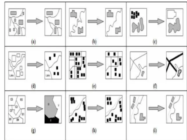
Figure 1: (a) Elimination, (b) Simplification, (c) Aggregation, (d) Size reduction, e) Typification, (f) Exaggeration, (g) Classification and
symbolisation, (h) Displacement, (i) Refinement.
The figure 1 shows different various operations involved in cartographic generalization. In this paper, we focus solely on simplification.
2. Cartographic Generalization and Some
Related Work
parametric buildings in aerial images. The simple simplification process simplify the object at a level after a level it will not produce better level of simplification. The basic simplification processes are effective only till a certain level, after which further improvement in results cannot be obtained, whereas the technique presented here provides the user options to simplify the object at various levels.
3. Multiple Representation v/s Cartographic
Generalization
Multilevel representation databases can quickly create maps at different scales (from predefined representations). However, they can not be considered an alternative to cartographic generalization [2]. A major drawback of multiple representation is that it often generates voluminous databases and restricts the cartographic products to the predefined scales. Many research projects have addressed multiple representation in multi-scale databases, in which every object has different representations at different scales. In these databases, an object has a detailed representation at a high scale, as well as a simplified representation at a low scale. This approach reduces the complexity of multiple representation, but does not solve the problem completely.
4. Simplification
When a map is represented graphically and the representation scale is reduced then some area features will become too insignificant to be represented, i.e. the object can be regularly or irregularly shaped. In this paper a simple approach has been presented to simplify contour lines and building plans to make the map more accurate and understandable. In this paper simplification for contour lines and buildings has been defined.
Vertex Simplification: Line simplification is also referred to as vertex simplification. Often a vertex has too much resolution for an application, such as visual displays of geographic map boundaries or detailed animated figures in games or movies. That is, the points on the vertexes representing the object boundaries are too close together for the resolution of the application. For example, in a computer display, successive vertices of the vertex may be displayed at the same screen pixel so that successive edge segments start, stay at, and end at the same displayed point. The whole figure may even have all its vertices mapped to the same pixel, so that it appears simply as a single point in the display. Different algorithms for reducing the points in a vertex to
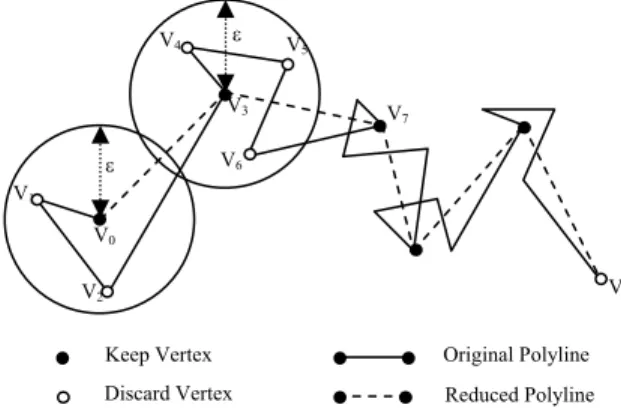
approximate the original within a specified tolerance have been purposed. Most of the algorithms work in any dimension since they only depend on computing the distance between points and lines. Thus, they can be applied to arbitrary 2D or 3D curves by sampling a parametric curve at regular small intervals. Vertex reduction is a brute-force algorithm for vertex simplification. Here a vertex is discarded when its distance from a prior initial vertex is less than some minimum tolerance ε > 0. More Specifically, after fixing an initial vertex V0, successive vertices Vi are tested and rejected if they are less than ε away from V0. But, when a vertex is found that is further away than ε, then it is accepted as part of the new simplified vertex, and it also becomes the new initial vertex for further steps of simplification. Thus, the resulting edge segments between accepted vertices are longer than the ε in length. This procedure is easily visualized as follows: [3]
Figure 2: Vertex Reduction used for Simplification
This is a fast first order O(n) algorithm. It should be implemented comparing squares of distances with the squared tolerance to avoid expensive square root calculations.
Here Douglas-Peucker (DP) approximation has been used to simplify the vertex in the map. This algorithm has O(nm) as worst case time, and O(nlogm) expected time, where m is the size of the simplified vertex. Note that this is an output dependent algorithm, and will be very fast when m is small. The first stage of the implementation does vertex reduction on the vertex before invoking DP approximation. This results in the well known vertex approximation/simplification algorithm which not only provides high quality results but is also very fast. Here the map information is provided by a server and the tolerance value is input by the user. The following steps are used to simplify the vertexes in the map.
V0
V1
V2
V3
V4 V5
V6
V7
V
Keep Vertex
Discard Vertex
Original Polyline
Algorithm:
Step [1]: Generate the Map.
Step [2]: Get the tolerance value from the user.
Step [3]: Calculate the number of objects or buildings on the screen.
Step [4]: Call the DOUGLAS PEUKAR recursive simplification routine to simplify the vertex.
Step [5]: Generate the simplified Map.
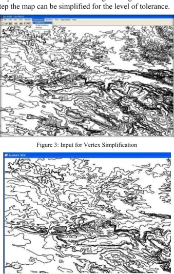
A sample contour data set from Survey of India (SoI)’s stored in Open Geo-spatial Consortium (OGC)’s Geography Markup Language (GML) format is used for simplification of line and buildings. Using the following step the map can be simplified for the level of tolerance.
Figure 3: Input for Vertex Simplification
Figure 4:Output file after Simplification process with tolerance value=5
Building Simplification: The main constraints involved in the simplification of building ground plans are preservation of right angles, co linearity and parallelism. Apart from preservation, enhancement of the characteristics may even be necessary. The deciding factor in simplification is the minimal length of a façade that can be represented at a certain scale. All the sides of building smaller than critical lengths have to be replaced.
The algorithm treats individual polygons one after the other. It works locally, trying to replace polygon sides which are shorter than the critical length. These sides are substituted according to some given rules, depending on the geometry of the adjacent building sides. This results in a simple, but not necessarily correct model of the original situation. Thus, in an adjustment process, the original building shape is adjusted to the new building model. The advantage of this procedure is the fact that the rules can be simple.
and coarse, as they yield only approximate values, which are refined in the adjustment process. Furthermore, additional parameters can also be introduced in the
Feature Feature Code
Major Code
Minor Code
Category Condition
Road RD 11 1100 Highway Metalled
11 1300 Motorway Metalled
11 5300 Motorway Unmetalled
11 6100 Pack-track
plains Unmetalled
11 6410
Cart-Track Plains
Unmetalled
11 6500 Foot-path
Plains Unmetalled
15 3000 Motorway Metalled
11 6300
Track follows Stream-bed
Unmetalled
Building Ntdb:00
000001 37 2100 Residential Block Village/Town
37 1100 Residential Hut Temporary
37 1200 Residential Hut Permanent
37 1400 Residential Hut Oblong Permanent
37 3020 Religious Chhatri
37 3040 Religious Idgah
adjustment, like the fact that the building size has to be preserved.
The first step of the algorithm results in a simplified ground plan, which is used as a model. This model is described in terms of building parameter that is in turn adjusted to the original ground plan in the subsequent adjustment process. The decision of how to substitute a short facade depends on the geometry of the neighboring sides:
Intrusion / extrusion: the angle between preceding and subsequent side is approx. 180 Æ. The small side is just set back to the level of the main facade.
Offset: the angle between preceding and subsequent side is approx. 0 Æ. The longer one of the adjacent building sides is extended, and the shorter side is dropped.
Corner: the angle between preceding and subsequent side is approx. 90 Æ. The adjacent facades are intersected. Following steps are to be followed for the simplification of the complete map.
Step [1]: Send a request for the GML to the server. Step [2]: Generate the Map.
Step [3]: Enter threshold value.
Step [4]: Calculate the number of objects or buildings on the screen.
Step [5]: Take the first object and follow the following steps for simplification.
Step [6]: OFFSET ANGLE – First rationalize the building to remove any offset angle.
Step [7]: Working in clockwise direction, take 3 consecutive points of the building and find the angle between them.
Step [8]: INTRUSION/EXTRUSION ANGLE – If the angle is greater than 190 degrees, this indicates the presence of either a protrusion or a corner in the building. Step [9]: A decision is made to ascertain whether a corner or a protrusion has been arrived at.
Step [10]: CORNER – If it’s a corner then we set the point as the meeting point of the two consecutive edges. Step [11]: PROTRUSION: we calculate its area and find out whether it is greater than the threshold area or not. If not, then the following steps are performed else the building is left unaltered.
Step [12]: If it’s a protrusion then store all the points in a temporary array till the angle formed by the 3 points is 180 degrees.
Step [13]:Follow the above steps from (7 to 12) till all the points are traversed.
Step [14]: Follow the above steps from (6 to 13) till all the objects are traversed.
Step [15]: Generate the final simplified Map.
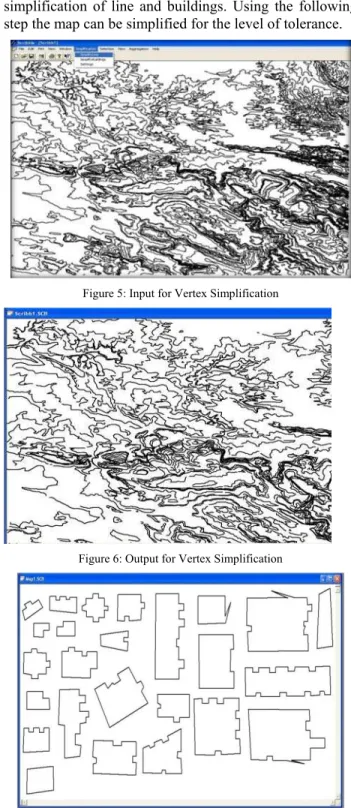
A sample contour data set from Survey of India (SoI)’s stored in Open Geo-spatial Consortium (OGC)’s Geography Markup Language (GML) format is used for simplification of line and buildings. Using the following step the map can be simplified for the level of tolerance.
Figure 5: Input for Vertex Simplification
Figure 6: Output for Vertex Simplification
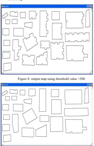
Figure 7: Input Building map for simplification process
Figure 8: output map using threshold value =500
Figure 9: output map using threshold value=1000
4. Conclusion
There are many approaches proposed for the process of vertex as well as polygon simplification. The technique proposed here modifies the existing technique to arrive at a more efficient model. The final map will be more accurate and understandable.
Acknowledgments
This research is being carried out under the project activity “Cartographic Generalization of Map Object’ sponsored by Department of Science & Technology (DST), India. This project is currently underway at Central Electronics Engineering Research Institute (CEERI), Pilani, India. Authors would like to thank Director, CEERI for his active encouragement and support and DST for the financial support.
References
[1] Robert Weibel and Christopher B. Jones, “Computational Perspective of Map Generalization”, GeoInformatica, vol. 2, pp 307-314, Springer Netherlands, November/December 1998.
[2] Brassel, K. E. and Robert Weibel, “A Review and framework of Automated Map Generalization”, International Journal of Geographical Information System, vol. 2, pp 229-224, 1988.
[3] M. Sester, ”Generalization Based on Least Squares Adjustment” International Archive of Photogrammetry and Remote Sensing, vol. 33, Netherland, 2000.
[4] Mathias Ortner, Xavier Descombes, and Josiane Zerubia, “Building Outline Extraction from Digital Elevation Models Using Marked Point Processes”, International Journal Computer vision, Springer, vol. 72, pp: 107-132, 2007.
[5] P. Zingaretti, E. Frontoni, G. Forlani, C. Nardinocchi, “Automatic extraction of LIDAR data classification rules”, 14th international conference on Image Analysis and Processing, pp 273-278, 10-14 Sept.
[6] Anders, K.-H. & Sester, M. [2000], Parameter-Free Cluster Detection in Spatial Databases and its Application to Typification, in: ‘IAPRS’, Vol. 33, ISPRS, Amsterdam, Holland. [7] Bobrich, J. [1996], Ein neuer Ansatz zur kartographischen Verdr ¨ angung auf der Grundlage eines mechanischen Feder-modells, Vol. C455, Deutsche Geod¨ atische Kommission, M¨ unchen.
[8] Bundy, G., Jones, C. & Furse, E. [1995], Holistic generalization of large-scale cartographic data, Taylor & Francis, pp. 106–119. [9] Burghardt, D. & Meier, S. [1997], Cartographic Displacement
Using the Snakes Concept, in: W. F¨ orstner & L. Pl ¨ umer, eds, ‘Smati ’97: SemanticModelling for the Acquisition of Topographic Information fromImages andMaps’, Birkh¨ auser, Basel, pp. 114–120.
[10] Douglas, D. & Peucker, T. [1973], ‘Algorithms for the reduction of the number of points required to represent a digitized line or its caricature’, The Canadian Cartographer 10(2), 112–122.
[11] Harrie, L. E. [1999], ‘The constraint method for solving spatial conflicts in cartographic generalization’, Cartographicy and Geographic Information Systems 26(1), 55–69.
[12] Hojholt, P. [1998], Solving Local and Global Space Conflicts in Map Generalization Using a Finite Element Method Adapted from Structural Mechanics, in: T. Poiker & N. Chrisman, eds, ‘Proceedings of the 8th International Symposium on Spatial Data handling’, Vancouver, Canada, pp. 679–689.
[13] J¨ ager, E. [1990], Untersuchungen zur kartographischen Symbolisierung und Verdr¨ angung im Rasterdatenformat, PhD thesis, Fachrichtung Vermessungswesen, Universit¨ at Hannover.
Dr. J. L. Raheja has received his M.Tech from IIT Kharagpur and PhD degree from Technical University Munich, Germany. At present he is Sr. Scientist in Central Electronics Engineering Research Institute (CEERI), Pilani, Rajasthan, since 2000. His area of interest is Cartographic Generalisation, digital image processing and Human Computer Interface.