Closed Form Solution to an Optimal Control Problem by Orthogonal Polynomial Expansion

ISSN 1941-7020

© 2008 Science Publications

Corresponding Author: Mohammad Ali Tavallaei, Department of Electrical Engineering, Urmia University, Urmia, Iran

Tel: +98-4413365779

Closed Form Solution to an Optimal Control Problem by

Orthogonal Polynomial Expansion

Mohammad Ali Tavallaei and Behrouz Tousi Department of Electrical Engineering,

Faculty of Engineering, Urmia University, Urmia, Iran

Abstract: In this study the use of orthogonal polynomials for obtaining a close form solution to optimal control problems with a weighed quadratic cost function, is proposed. The method consists of using the Orthogonal Polynomials for the expansion of the state variables and the control signal. This expansion results in a set of linear equations, from which the closed form solution is obtained. A numerical example is provided to demonstrate the applicability and effectiveness of the proposed method.

Key words: Optimal control, orthogonal polynomials, spectral method, legendry polynomials, riccati method

INTRODUCTION

The goal of an optimal controller is the determination of the control signal such that a specified performance criterion is optimized, while at the same time specific physical constraints are satisfied. Many different methods have been introduced to solve such a problem for a system with given state equations. The most popular is the Riccati method for quadratic cost functions however this method results in a set of usually complicated differential equations which must be solved recursively[1]. In the last few decades orthogonal functions have been extensively used in obtaining an approximate solution of problems described by differential equations[2-4]. The approach, also known as the spectral method[5], is based on converting the differential equations into an integral equation through integration. The state and/or control involved in the equation are approximated by finite terms of orthogonal series and using an operational matrix of integration to eliminate the integral operations. The form of the operational matrix of integration depends on the particular choice of the orthogonal functions like Walsh functions[6], block-pulse functions[7], Laguerre series[8], Jacobi series[9-10], Fourier series[11], Bessel series[12], Taylor series[13], shifted Legendry[14], Chebyshev polynomials[15] and Hermit polynomials[16] and Wavelet functions[17]. In this study apart from the shifted Legendry Polynomials, new set of Orthogonal Polynomials are considered based on the requirement of the problem. This method

proves to be fairly precise from simulation results and may be expanded to a vast range of cost functions.

Since only linear systems are considered in this study, the state space equations and the cost function are considered in the following formats:

) t ( Bu ) t ( AX

X= +

•

(1)

In which A and B are constant matrices. And the cost function:

∫

+

= f

t

0

2 T

k

dt )] t ( ru ) t ( QX ) t ( X t [ 2 1

J (2)

In which Q is a positive definite matrix and r and k are constant values. tf is the final time and specified.

105 Solving optimal control problems by the use of orthogonal polynomials: In the presented method,

) t (

u and X(t) must be expanded based on orthogonal polynomials in order to solve the optimal control problem. However due to the presence of the term tk in J, X(t) may not be presented by the shifted Legendry Polynomials. In order to solve this problem, weighed orthogonal polynomials with the weighting function tk, are defined which will be represented withϕi(t). Then X(t) is expanded based on these new orthogonal polynomials {ϕi(t)}. Some of the characteristics of orthogonal functions are recapitulated next.

Orthogonal polynomials: The definition of orthogonal polynomials ψn(t) and some of their features are presented below:

j i

j i 0 dt ) t ( ) t ( ) t ( W

b

a

i j

i _≠

=   χ = ψ ψ

∫

(3)

In which W(t) is the weight function.

The expansion of an arbitrary function f(t) on the ]

t , 0

[ f region is as follows:

∑

= ψ

= N 0 i Ci i(t)

) t (

f (4)

In which:

∫

ψ

χ = f

t

0 i k

i

i tf(t) (t)dt

1

C (5)

One property of orthogonal polynomials is[19]:

∫

ψ(t)=κψ(t) (6)

Now for a weight function W(t)=1, we have the shifted Legendre polynomials:

)} t ( { )} t ( P

{ _i = ψ_i (7)

and

∫

f =γ

t

0 T

dt

PP (8)

In which:

T n 1

0(t),P(t),...,P(t)]

P [ ) t (

P = (9)

] ,..., , [

diagγ0 γ1 γn

=

γ (10)

∫

= γ f

t

0 2 i

i P (t)dt (11)

Now for a weight function k

t ) t (

W = , we define the polynomials {ϕ_i(t)} shown below:

)} t ( { )} t ( {ϕi = ψi

∫

f ϕϕ =α

t

0 T k

dt

t (12)

In which:

T n 1

0(t), (t),..., (t)]

[ϕ ϕ ϕ

=

ϕ (13)

] ,..., , [

diagα0α1 αn

=

α (14)

∫

ϕ = α f

t

0 2 i k

i t (t)dt (15)

The integral expansion of the weighed orthogonal polynomials ϕi(t) based on the set {ϕi(t)} is as follows:

∫

tϕ ≅ ϕ

0

D

dt (16)

The method for obtaining D is explained in the appendix.

It is worth noting that when dealing with functions and their derivatives, the property mentioned in Eq. 16 is of major importance.

Obtaining orthogonal polynomials: Different methods may be used to obtain orthogonal polynomials, namely, most commonly, the Graham-Schmidt method[18]. However this method is computationally cumbersome for large sets and may produce inaccurate results. Here, another method is introduced which is based on the properties of orthogonal polynomials, for W(t) = tk. The presented method is computationally effective and precise compared to the Graham Schmidt method due to the fact that approximations in numerical integration needed for the Graham Schmidt method are not required for the presented method. It is assumed that:

Hence:

T t

0

t

0

t

0

T T k T

k T k

SYS S ) dt TT t ( S dt STT t dt t

f f f

∫

ϕϕ =

∫

=

∫

= (18)

In which:

T n 1 0

] t ,..., t , t [ T= and

) 1 n ( ) 1 n ( 1 n 2 K f 2

n K f 1 n K f

1 n K f 2

K f 1

K f

1 n 2 K

t 2

n K

t 1 n K

t

1 n K

t 2

K t 1 K

t

Y

+ × + + + +

+ +

+

+ + +

+

      

 

      

 

+ + +

+ + +

+ + +

+ =

L M M

M

M M

M

L

(19)

Now because Y is real symmetrical and positive definite it can be transformed to the form below by the cholesky method:

Y = LLT (20)

Now based on the definition of orthogonal polynomials, we can assume that:

SYST = 1 (21)

In which I is an (n+1)×(n+1) identity matrix. This would mean that:

S = L−1 (22)

So we can now obtain S and finally ϕ = ST.

Formulation of an optimal control problem using weighed orthogonal polynomials: Now the optimal control problem described by Eq. 1 and 2 is formulized by the use of the orthogonal polynomials. First

) t ( xi

•

will be expanded based on the set {ϕi(t)} up to degree n:

ϕ ≅ ⇒ ϕ

= •

•

E X e x

T

i

i (23)

In which:

1 m m 1

) 1 n ( m mn 1

m 0 m

n 1 11 10

) t ( x

. . . ) t ( x X e

... e e

. . . ... . . .

. . .

e ... e e E

× +

×

    

 

    

 

=

    

 

    

 

= (24)

Where, m is the order of the system. It must be noted that E is unknown and will be obtained later on.

And u(t) the control signal will be expanded based on the set {Pi(t)} up to degree n:

P u_=βT

(25) In which:

T ) 1 n ( 1 n 1 0, ,..., ]

[β β β _{× +} =

β

Note that each of the functions Pi(t) may be expanded based on the set {ϕi(t)} or vice versa in Eq. 24. Therefore we have:

ϕ = T

c

P (26)

In which c is a (n+1)×(n+1) square matrix. Substituting into Eq. 25 we have:

ϕ β = T T

c

u (27)

βis also unknown and will be obtained later on. Now by the use of Eq. 16, 23 and 27 we can write:

ϕ + = ⇒ + ϕ

=ED VP X (ED Vc )

X T

(28) In which:

) 1 n ( m 0

m 10

0 ... 0 0 x

. ... . . .

. ... . . .

. ... . . .

0 ... 0 0 x

V

+ ×

     

 

     

 

= (29)

where, xi0 in Eq. 29 is the initial condition for the state variable xi(t). By replacing Eq. 23, 27 and 28 in to the state Eq. 1 we have:

ϕ β + ϕ + =

ϕ T T T

c B ) Vc ED ( A

E (30)

Therefore the following equation holds for all values of t:

0 c B ) Vc ED ( A

E− + T − β T=

(31) And the matrix I may be defined as:

] ) c B ) Vc ED ( A E [( Vec

I₌∆ _{− +} T _{− β} T T

107 So I = 0.

By replacing the expansions for u and X as formulated in Eq. 31 and 32 respectively, in the expression for J in Eq. 2 we have:

∫

∫

γβ β + ϕ + + ϕ = f f t 0 T T T T t 0 T k dt r 2 1 ... dt ) Vc ED ( Q ) Vc ED ( t 2 1 J (33)

By the use of the properties of orthogonal functions )

t (

P_i and ϕ_i(t), the functional J takes the simpler form of: } r ... )] Vc ED ( Q ] Vc ED ( [ trace { 2 1 J T T T γβ β + + + α = (34)

For minimizing J with the restriction in Eq. 32 or 30 we can use the Lagrange coefficients and minimize the following expression instead:

) , E ( I . ) , E ( J ) , , E

( _{βλ = β +λ}T _β

η (35)

In which λ is the Lagrange coefficient and:

T n m 1 0, ,..., ]

[λ λ λ _× =

λ (36)

Now η(E,β,λ) must be minimized, which is done by solving the following equations:

0 eij = ∂ η ∂ , 0 i = β ∂ η ∂

, 0

i = λ ∂ η ∂ (37)

After performing the above differentiations and simplification[19], the following important equations are obtained: ) D D ( Q 2 ) E ( vec ) QED E D ( trace T T T T α ⊗ = ∂ α ∂ (38) λ ⊗ = ∂ λ ∂ ) D A ( ) E ( vec ) A E D ( vec . T T T T T T (39) ) Q cV D ( vec ) E ( vec ) QVc E D ( trace T T T T T α = ∂ α ∂ (40) ) A E D ( vec ) A E D ( vec

. T T T

T T T T = λ ∂ λ ∂ (41) ) E ( vec ). D A ( ) A E D (

vec T T T _{= ⊗} T T

(42) And the set of linear equations are finally obtained:

        

− α

=           λ β           ⊗ − γ ⊗ − ⊗ − ⊗ − α ⊗ 0 ] A cV [ Vec ] Q cV D [ Vec ) E ( Vec c B r 0 0 c B D A I D A I 0 ) D D ( Q T T T T T T T T T (43)

In which ⊗ is the symbol of Kronecker multiplication and by Vec(matrix) we mean placing the columns of the matrix in consecutive order in one vector.

The unknown variablesλi, βiand eij in 37 are of

first order and hence are easily obtainable from solving the linear set of Eq. in 43. By solving the set of linear Eq. in 43 the coefficients eij and βi which were used in

the expansions represented in Eq. 25 and 28 are obtained. Therefore we have now obtained the following solution to our original problem:

P u_=βT

, X=EDϕ+VP (44)

A numerical example: In this research the result formulated in Eq. 43 is applied and compared with the result of the classical Riccati method for a specific system with the following specifications:

      − = 1 1 0 2

A , 

     = 1 0

B , 

     = 2 0 0 1 ) t (

Q , r=0.5 (45)

And we wish to minimize the cost function:

∫

+ = f t 0 2 T k dt )] t ( ru ) t ( X ) t ( Q ) t ( X t [ 2 1

J (46)

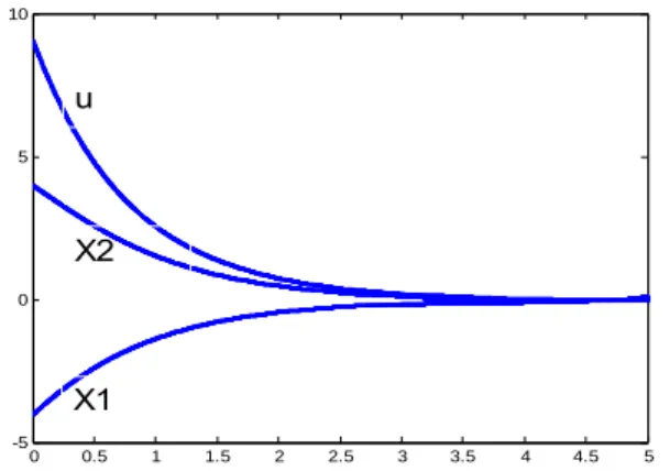
The problem is solved for k=0and k=3, with n = 9. The results are shown in Fig. 1 and 2 respectively.

0 0.5 1 1.5 2 2.5 3 3.5 4 4.5 5 -5 0 5 10 u X1 X2

Fig. 1: Depicted numerical results for k = 0, n = 9 of both the presented method and that of the Riccati method

0 0.5 1 1.5 2 2.5 3 3.5 4 4.5 5

-6 -4 -2 0 2 4 6 8 10 12 u X1 X2

Fig. 2: Depicted numerical results for k=3,n=9, of both the presented method and that of the Riccati method. 000000 . 4 t 952058 . 2 t 241816 . 0 t 353073 . 1 t 853478 . 0 t 277442 . 0 t ) 10 513299 . 0 ( t ) 10 507526 . 0 ( t ) 10 204330 . 0 ( t ) 10 257824 . 0 ( X 2 3 4 5 6 1 7 2 8 3 9 6 2 + − − + − + × − × + × − × − = − − − − 047942 . 9 t 43569 . 11 t 769460 . 6 t 899631 . 1 t 142803 . 0 t 310854 . 0 t 108283 . 0 t ) 10 181063 . 0 ( t ) 10 147546 . 0 ( t ) 10 450041 . 0 ( u 2 3 4 5 6 7 1 8 2 9 4 + − + − − + − × + × − × = − − −

For tf=5, k = 3 and n = 9 the following solutions are obtained: 000000 . 4 t 000000 . 4 t 845372 . 0 t 180791 . 0 t 198410 . 0 t 271386 . 0 t 112345 . 0 t ) 10 228522 . 0 ( t ) 10 234829 . 0 ( t ) 10 978057 . 0 ( X 2 3 4 5 6 7 1 8 2 9 4 1 − + − − − + − × + × − × = − − − 000000 . 4 t 690745 . 1 t 542373 . 0 t 793643 . 0 t 356930 . 1 t 674073 . 0 t 159966 . 0 t ) 10 187863 . 0 ( t ) 10 880251 . 0 ( t ) 10 865658 . 0 ( X 2 3 4 5 6 7 1 8 3 9 8 2 + − − − + − + × − × + × = − − − 30925 . 10 t 77549 . 10 t 232559 . 1 t 99565 . 4 t 616614 . 1 t 257048 . 0 t 253152 . 0 t ) 10 574488 . 0 ( t ) 10 557675 . 0 ( t ) 10 195626 . 0 ( u 2 3 4 5 6 7 1 8 2 9 3 + − − + − − + × − × + × − = − − − CONCLUSION

In this study we have presented an alternative method for obtaining an analytical approximate solution to optimal control problems with time variant weight in the cost function. The presented method makes use of the properties of orthogonal polynomials and transforms the problem into a linear set of equations. The results of the presented method proved to be accurate by comparison with that of the classical riccati method.

REFERENCES

1. Kirk, D., 1970. Optimal Control Theory: An Introduction. Prentice-Hall, Englewood Cliffs, NJ.

1st edition, ISBN 9780136380986

2. Sadek, I. and M. Bokhari, 1998. Optimal control of a parabolic distributed parameter system via orthogonal polynomials. Optimal Control Appl. Methods, 19: 205-213.

3. Chang, R. and S. Yang, 1986. Solutions of two-point-boundary-value problems by generalized orthogonal polynomials and applications to control of lumped and distributed parameter systems. Int. J. Control, 43: 1785-1802.

4. Razzaghi, M. and A. Arabshahi, 1989. Optimal control of linear distributed parameter systems via polynomial, series. Int. J. Syst. Sci., 20: 1141-1148. 5. Alipanah, A., M. Razzaghi and M. Dehgan, 2007. Non-classical pseudospectral method for the solution of brachistochrone problem. Chaos Solut. Fract., 34: 1622-1628.

6. Chen, C.F. and C.H. Hsiaso, 1965. A state-space approach to walsh series solutions of linear systems. Int. J. Syst. Sci., 6: 833-858.

7. Hsu, N.S. and B. Cheng, 1981. Analysis and optimal control of time varying linear systems via block-pulse functions. Int. J. Control, 33: 1107-1122.

109 9. Razzaghi, M., 1989. Shifted jacobi series direct

method for variation n problems. Int. J. Syst. Sci., 20: 1119-1129.

10. Liu, C. and Y. Shin, 1985. System analysis, parameter estimation and optima regular design of linear systems via jacobi series. Int. J. Control, 38: 211-223.

11. Yang, C. and C. Chen, 1994. Analysis and optimal control of time-varying linear systems via fourier series. Int. J. Syst. Sci., 25: 1663-1678.

12. Parashevopoulos, P.N., P. Skavounos and G.Gh. Georgiou, 1990. The operation matrix of integration for bessel functions. J. Franklin Inst., 330: 329-341.

13. Razzaghi, M., 1988. Taylor series direct method for variation problems. J. Franklin Inst. 325: 125-131.

14. Razzaghi, M. and G. Elnager, 1993. A legendre technique for solving time-varying linear quadratic optimal control problems. J. Franklin Inst., 330: 1-6.

15. Nagurka, M.L. and S. Wang, 1993. A chebyshev-based state representation for linear quadratic optimal control. Trans. ASME Dynam. Syst. Meas. Control, 115: 1-6.

16. Wedig, W., Kree, P., 1995. Probabilistc Methods in Applied Physics, Springer Berlin, ISBN 9783540602149

17. Sadek, I., T. Abualrub and M. Abukhaled, 2007. A computational method for solving optimal control of a system of parallel beams using legendre wavelets. Math. Comput. Model., 45: 11253-1264. 18. Kreyszig, E., 1999. Advanced Engineering

Mathematics. John Wiley and Sons Inc, 8th edition, New York, ISBN 047133328