J. Braz. Comp. Soc. vol.14 número3

Automatic Music Genre

Classification

Carlos N. Silla Jr.

, Alessandro L. Koerich

and Celso A. A. Kaestner

1_{University of Kent – Computing Laboratory}

Canterbury, CT2 7NF Kent, United Kingdom

cns2@kent.ac.uk

2_{Pontifical Catholic University of Paraná}

R. Imaculada Conceição 1155, 80215-901 Curitiba - Paraná - Brazil

alekoe@ppgia.pucpr.br

3_{Federal University of Technology of Paraná}

Av. Sete de Setembro 3165, 80230-901 Curitiba - Paraná - Brazil celsokaestner@utfpr.edu.br

Received 06 January 2008; accepted 23 July 2008

Abstract

This paper presents a non-conventional approach for the automatic music genre classification problem. The proposed approach uses multiple feature vectors and a pattern recognition ensemble approach, according to space and time decomposition schemes. Despite being music genre classification a multi-class problem, we ac-complish the task using a set of binary classifiers, whose results are merged in order to produce the final music genre label (space decomposition). Music segments are also decomposed according to time segments obtained from the beginning, middle and end parts of the original music signal (time-decomposition). The final classifica-tion is obtained from the set of individual results, accord-ing to a combination procedure. Classical machine learn-ing algorithms such as Naïve-Bayes, Decision Trees, k Nearest-Neighbors, Support Vector Machines and Multi-Layer Perceptron Neural Nets are employed. Experiments were carried out on a novel dataset called Latin Music Database, which contains 3,160 music pieces categorized in 10 musical genres. Experimental results show that the proposed ensemble approach produces better results

than the ones obtained from global and individual seg-ment classifiers in most cases. Some experiseg-ments related to feature selection were also conducted, using the genetic algorithm paradigm. They show that the most important features for the classification task vary according to their origin in the music signal.

Keywords: music genre classification, machine learn-ing, pattern classification, feature selection.

1. I

Music is nowadays a significant part of the Internet content: the net is probably the most important source of music pieces, with several sites dedicated to spread-ing, distributing and commercializing music. In this con-text, automatic procedures capable of dealing with large amounts of music in digital formats are imperative, and Music Information Retrieval (MIR) has become an im-portant research area.

ex-perts in order to identify the style of the music. The music genre is a descriptor that is largely used to organize col-lections of digital music. It is not only a crucial metadata in large music databases and electronic music distribution (EMD) [1], but also the most frequent item used in search queries, as pointed by several authors [8], [20], [30], [35], [36].

Up to now the standard procedure for organizing music content is the manual use of meta information tags, such as the ID3 tags associated to music coded in MPEG-1 Audio Layer 3 (MP3) compression format [15]. This metadata includes song title, album, year, track num-ber and music genre, as well as other specific details of the file content. The music genre information, however, is usually incomplete and inaccurate, since it depends on human subjectiveness. As there is no industrial standard, more confusion arises: for example, the same music piece is indicated as belonging to different music genres accord-ing to different EMD sites, due to different interpretation and/or different codification schemes [19].

We emphasize that AMGC also poses an interesting research problem from a pattern recognition perspective. Music can be considered as a high-dimensional digital time-variant signal, and music databases can be very large [2]; thus, it offers a good opportunity for testing non-conventional pattern recognition approaches.

As each digital music segment can be associated to a vector representative, by applying some extracting proce-dure to calculate appropriate feature values, to put this problem as a classical classification task in the pattern recognition framework is straightforward [28]. Typically a music database (as in a EMD) contains thousands of pieces from dozens of manually-defined music genres [1], [23], [32] characterizing a complex multi-class problem.

In this paper we present a non-conventional machine learning approach to the AMGC problem. We use the en-semble approach [7], [17] based on bothspaceandtime

decomposition schemes. Firstly, the AMGC problem is naturally multi-class; as pointed in the literature [7], [12], inter class similarity / extra class distinction are inversely proportional to the number of classes involved. This sit-uation can be explained by considering that is difficult to most classifiers to construct an adequate separation sur-face among the classes [24]. One solution is to decom-pose the original multi-class problem space as a series of binary classification problems, where most of the known classifiers work better, and to merge the obtained results in order to produce the final result. Secondly, as music is a time-varying signal, several segments can be employed to extract features, in order to produce a set of feature vectors that characterizes a decomposition of the original signal according to the time dimension. We employ an en-semble approach that encompasses both decompositions: classifiers are applied to space-time partial views of the

music, and the obtained classification results are merged to produce the final class label.

We also conduct some experiments related to feature selection, employing a genetic algorithm framework, in order to show the relation between the relative importance of each feature and its origin in the music signal.

This paper is organized as follows: section 2 presents a formal view of the problem and summarize the results of several research works in automatic music genre classifi-cation; section 3 presents our proposal, based on space-time decomposition strategies, describing also the em-ployed features, classification and results combination al-gorithms; section 4 presents the employed dataset and the experimental results obtained with the space-time decom-position; section 5 describes the employed feature selec-tion procedure, and the obtained experimental results; fi-nally, section 6 presents the conclusions of our work.

2. P

Nowadays the music signal representation is no longer analogous to the original sound wave. The analogical sig-nal is sampled, several times per second, and transformed by an analogous-to-digital converter into a sequence of numeric values in a convenient scale. This sequence rep-resent the digital audio signal of the music, and can be employed to reproduce the music [15].

Hence the digital audio signal can be represented by a sequenceS =< s1, s2. . . sN >wheresi stands for the

signal sampled in the instant iandN is the total num-ber of samples of the music. This sequence contains a lot of acoustic information, and features related to timbral texture, rhythm and pitch content can be extracted from it. Initially the acoustic features are extracted from short frames of the audio signal; then they are aggregated into more abstract segment-level features [2]. So a feature vec-torX¯ =< x1, x2. . . xD>can be generated, where each

featurexj is extracted fromS (or some part of it) by an

appropriate extraction procedure.

Now we can formally define the AMGC problem as a pattern classification problem, using segment-level fea-tures as input. From a finite set of music genres G we must select one classgˆwhich best represents the genre of the music associated to the signalS.

From a statistical perspective the goal is to find the most likelygˆ∈ G, given the feature vectorX¯, that is

ˆ

g=argmax

g∈GP(g|

¯ X)

whereP(g|X¯)is thea posterioriprobability that the mu-sic belong to the genreggiven the features expressed by

¯

X. Using the Bayes’ rule the equation can be rewritten as

ˆ

g=argmax

g∈G

whereP( ¯X|g)is the probability in which the feature vec-torX¯ occurs in classg,P(g)is thea prioriprobability of the music genreg(which can be estimated from frequen-cies in the database) andP( ¯X)is the probability of oc-currence of the feature vectorX¯. The last probability is in general unknown, but if the classifier computes the likeli-hoods of the entire set of genres, thenPg∈GP(g|X¯) = 1 and we can obtain the desired probabilities for eachg∈ G

by

P(g|X¯) = PP( ¯X|g).P(g)

g∈GP( ¯X|g).P(g)

The AMGC problem was initially defined in the work of Tzanetakis and Cook [35]. In this work a compre-hensive set of features was proposed to represent a mu-sic piece. These features are obtained from a signal pro-cessing perspective, and include timbral texture features, beat-related features and pitch-related features. As clas-sification procedures they employ Gaussian classifiers, Gaussian mixture models and the k Nearest-Neighbors (k-NN) classifier. The experiments occur in a database called GTZAN, that include 1,000 samples from ten music genres, with features extracted from the first30 -seconds of each music. Obtained results indicate an accu-racy of about 60% using a ten-fold cross validation pro-cedure. The employed feature set has become of public use, as part of the MARSYAS framework (Music Analy-sis, Retrieval and SYnthesis for Audio Signals, available at http://marsyas.sourgeforge.net/), a free software plat-form for developing and evaluating computer audio ap-plications [35].

Kosina [19] developed MUGRAT (MUsic Genre Recognition by Analysis of Texture, available at http://kyrah.net/mugrat), a prototypical system for mu-sic genre recognition based on a subset of the features given by the MARSYAS framework. In this case the fea-tures were extracted from3-second segments randomly selected from the entire music signal. Experiments were carried out in a database composed by186music samples belonging to 3 music genres. Employing a3-NN clas-sifier Kosina obtains an average accuracy of88.35% us-ing a ten-fold cross-validation procedure. In this work the author also confirms that manually-made music genre classification is inconsistent: the very same music pieces obtained from different EMD sources were differently la-beled in their ID3 genre tag.

Li, Ogihara and Li [21] present a comparative study between the features included in the MARSYAS frame-work and a set of features based on Daubechies Wavelet Coefficient Histograms (DWCH), using also other classi-fication methods such as Support Vector Machines (SVM) and Linear Discriminant Analysis (LDA). For compari-son purposes they employ two datasets: (a) the original dataset of Tzanetakis and Cook (GTZAN), with features

extracted from the beginning of the music signal, and (b) a dataset composed by755music pieces of5music genres, with features extracted from the interval that goes from second 31 to second 61. Conducted experiments show that the SVM classifier outperforms all other methods: in case (a) it improves accuracy to72% using the origi-nal feature set and to78%using the DWCH feature set; in case (b) the results were71%for the MARSYAS fea-ture set and74% to the DWCH feature set. The authors also evaluate some space decomposition strategies: the original multi-class problem (5classes) was decomposed in a series of binary classification problems, according to a One-Against-All (OAA) and Round-Robin (RR) strate-gies (see Section 3.1). The best results were achieved with SVM and OAA space decomposition using DWCH fea-ture set. Accuracy was improved by2to7%according to employed feature set – DWCH and MARSYAS respec-tively – in the dataset (a), and by2to4%in dataset (b).

Grimaldi, Cunningham and Kokaram [13], [14] em-ploy a space decomposition strategy to the AMGC prob-lem, using specialized classifiers for each space vision and an ensemble approach to obtain the final classifica-tion decision. The authors decompose the original prob-lem according to OAA, RR – called pairwise compari-son [12] – and random selection of subspaces [16] meth-ods. They also employ different feature selection proce-dures, such as ranking according to information gain (IG) and gain ratio (GR), and Principal Component Analysis (PCA). Experiments were conducted in a database of200

music pieces of5music genres, using thek-NN classifier and a 5-fold cross validation procedure. The feature set was obtained from the entire music piece, using discrete wavelet transform (DPWT). Fork-NN classifier the PCA analysis proves to be the most effective feature selection technique, achieving an accuracy of79%. The RR ensem-ble approach scores81%for both IG and GR, showing to be an effective ensemble technique. When applying a for-ward sequential feature selection based on the GR rank-ing, the ensemble scores84%.

better results for classification.

Yaslan and Catalpete [38] employ a large set of clas-sifiers to study the problem of feature selection in the AMGC problem. They use the linear and quadratic dis-criminant classifiers, the Naïve-Bayes classifier, and vari-ations of thek-NN classifier. They employ the GTZAN database and the MARSYAS framework [35] for fea-ture extraction. The feafea-tures were analyzed according to groups, for each one of the classifiers. They employ the Forward Feature Selection (FFS) and Backward Feature Selection (BFS) methods, in order to find the best feature set for the problem. These methods are based on guided search in the feature space, starting from the empty set and from the entire set of features, respectively. They re-port positive results in the classification with the use of the feature selection procedure.

Up to now most researchers attack the AMGC prob-lem by ensemble techniques using only space decompo-sition. We emphasize that these techniques employ dif-ferent views of the feature space and classifiers dedicated to these subspaces to produce partial classifications, and a combination procedure to produce the final class label. Furthermore the features used in these works are selected from one specific part of the music signal or from the en-tire music signal.

One exception is the work of Bergstra et al. [2]. They use the ensemble learner AdaBoost [11] which performs the classification iteratively by combining the weighted votes of several weak learners. Their model uses sim-ple decision stumps, each of which operates on a sin-gle feature dimension. The procedure shows to be effec-tive in three music genre databases (Magnatune, USPOP and GTZAN), winning the music genre identification task in the MIREX 2005 (Music Information Retrieval EX-change) [9]. Their best accuracy results vary from75to

86%in these databases.

The first work that employs time decomposition us-ing regular classifiers applied to complete feature vectors was proposed by Costa, Valle Jr. and Koerich [4]. This work presents experiments based on ensemble of classi-fiers approach that uses three time segments of the music audio signal, and where the final decision is given by the majority vote rule. They employ a MLP neural net and thek-NN classifiers. Experiments were conducted on a database of414music pieces of2genres. However, final results regarding the quality of the method for the clas-sification task were inconclusive. Koerich and Poitevin [18] employ the same database and an ensemble approach with a different set of combination rules. Given the set of individual classifications and their corresponding score – a number associated to each class also obtained from the classification procedure – they use the maximum, the sum and pondered sum, product and pondered product of the scores to assign the final class. Their experiments show

better results than the individual classifications when us-ing two segments and the pondered sum and the pondered product as result combination rules.

3. T

-

In this paper we evaluate the effect of using the en-semble approach in the AMGC problem, where individ-ual classifiers are applied to a special decomposition of the music signal that encompasses both space and time di-mensions. We use feature space decomposition following the OAA and RR approaches, and also features extracted from different time segments [31], [33], [34]. Therefore several feature vectors and component classifiers are used in each music part, and a combination procedure is em-ployed to produce the final class label for the music.

3.1. SPACE DECOMPOSITION

Music genre classification is naturally a multi-class problem. However, we employ a combination of the re-sults given by binary classifiers, whose rere-sults are merged afterwards in order to produce the final music genre label. This procedure characterizes a space decomposition

of the feature space, since features are used according to different views of the problem space. The approach is jus-tified because for two class problems the classifiers tend to be simple and effective. This point is related to the type of the separation surface constructed by the classi-fier, which are limited in several cases [24].

Two main techniques are employed to produce the de-sired decomposition: (a) in theone-against-all(OAA) ap-proach, a classifier is constructed for each class, and all the examples in the remaining classes are considered as negative examples of that class; and (b) in theround-robin

(RR) approach, a classifier is constructed for each pair of classes, and the examples belonging to the other classes are discarded. Figures 1 and 2 schematically illustrate these approaches. For aM-class problem (Mmusic gen-res) several classification results arise: according to the OAA techniqueM class labels are produced, whereas for the RR technique M(M −1)/2 class labels are gener-ated. These labels are combined according to a decision procedure in order to produce the final class label.

Figure 1. One-Against-All Space Decomposition Approach

Figure 2. Round-Robin Space Decomposition Approach

3.2. TIME DECOMPOSITION

An audio record of a music piece is a time-varying signal. The idea behindtime decomposition is that we can obtain a more adequate representation of the music piece if we consider several time segments of the sig-nal. This procedure aims to better treat the great variation that usually occurs along music pieces, and also permits to compare the discriminative power of the features ex-tracted from different parts of the music.

Figure 3 illustrates this point: it presents the aver-age values of 30 features extracted from different mu-sic sub-intervals, obtained over 150 mumu-sic pieces of the genre Salsa. We emphasize the irregularity of the results, showing that feature values vary depending on the interval from which they were obtained.

If we employ the formal description of the AMGC problem given in the previous section, the time decompo-sition can be formalized as follows. From the original mu-sic signalS =< s1, s2. . . sN >we obtain different

sub-signalsSpq. Each sub-signal is simply a projection ofS

on the interval[p, q]of samples, orSpq=< sp, . . . sq >.

In the generic case that usesK sub-signals, we further

Figure 3. Average values over 150 music pieces of genre Salsa for 30 features extracted from different music sub-intervals

obtain a sequence of feature vectorsX¯1,X¯2. . .X¯K. A

classifier is applied in each one of these feature vectors, generating the assigned music genresˆg1,gˆ2. . .gˆK; then

they must be combined to produce the final class assign-ment, as we will see in the following.

In our case we employ feature vectors extracted from 30-seconds segments from the beginning (Sbeg), middle

(Smid) and end (Send) parts of the original music

sig-nal. The corresponding feature vectors are denotedX¯beg,

¯

XmidandX¯end. Figure 4 illustrates the time

decomposi-tion process.

Figure 4. Time Decomposition Approach

3.3. THE SET OF EMPLOYED FEATURES

Texture:19; Pitch:5). For a more detailed description of the features refer to [34] or [35] .

A normalization procedure is applied, in order to ho-mogenize the input data for the classifiers: ifmaxV and

minV are the maximum and minimum values that appear in all dataset for a given feature, a valueV is replaced by

newV using the equation

newV = (V −minV) (maxV −minV)

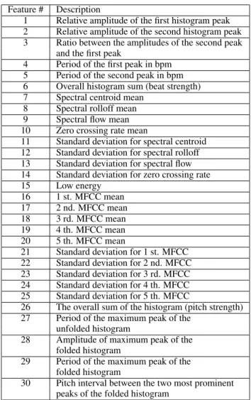
The final feature vector is outlined in Table 1.

Table 1. Feature vector description

Feature # Description

1 Relative amplitude of the first histogram peak 2 Relative amplitude of the second histogram peak 3 Ratio between the amplitudes of the second peak

and the first peak

4 Period of the first peak in bpm 5 Period of the second peak in bpm 6 Overall histogram sum (beat strength) 7 Spectral centroid mean

8 Spectral rolloff mean 9 Spectral flow mean 10 Zero crossing rate mean

11 Standard deviation for spectral centroid 12 Standard deviation for spectral rolloff 13 Standard deviation for spectral flow 14 Standard deviation for zero crossing rate 15 Low energy

16 1 st. MFCC mean 17 2 nd. MFCC mean 18 3 rd. MFCC mean 19 4 th. MFCC mean 20 5 th. MFCC mean

21 Standard deviation for 1 st. MFCC 22 Standard deviation for 2 nd. MFCC 23 Standard deviation for 3 rd. MFCC 24 Standard deviation for 4 th. MFCC 25 Standard deviation for 5 th. MFCC

26 The overall sum of the histogram (pitch strength) 27 Period of the maximum peak of the

unfolded histogram

28 Amplitude of maximum peak of the folded histogram

29 Period of the maximum peak of the folded histogram

30 Pitch interval between the two most prominent peaks of the folded histogram

We note that the feature vectors are always calculated over intervals; in fact several features like means, vari-ances, and number of peaks, only have meaning if ex-tracted from signal intervals. So they are calculated over

Sor one of its subintervalsSpq, that is, an aggregate

seg-ment obtained from the eleseg-mentary frames of the music audio signal.

3.4. CLASSIFICATION AND COMBINATION DECI

-SION PROCEDURES

A large set of standard algorithms for supervised ma-chine learning is used to accomplish the AMGC task. We follow an homogeneous approach, that is, the very same classifier is employed as individual component classifier in each music part. We use the following algorithms [28]: (a) a classic decision tree classifier (J48); (b) the instance-basedk-NN classifier; (c) the Naïve-Bayes clas-sifier (NB), which is based on conditional probabilities and attribute independence; (d) a Multi Layer Perceptron neural network (MLP) with the backpropagation momen-tum algorithm; and (e) a Support Vector Machine classi-fier (SVM) with pairwise classification. In order to do all experiments we employ a framework based on the WEKA Datamining Tool [37], with standard parameters.

As previously mentioned, a set of possibly different candidate classes is produced by the individual classi-fiers. These results can be considered according to space and time decomposition dimensions. The time dimension presentsKclassification results, and space dimension for aM-class problem producesM (OAA) orM(M−1)/2

(RR) results, as already explained. These partial results must be composed to produce the final class label.

We employ a decision procedure in order to find the final class associated by the ensemble of classifiers. Space decomposition results are combined by the majority vote rule, in the case of the RR approach, and by a rule based on thea posterioriprobability of the employed classifier, for the OAA approach. Time decomposition results are combined using the majority vote rule.

4. S

-

-PERIMENTS AND RESULTS

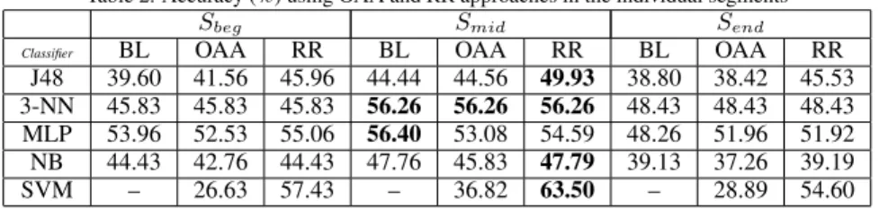
Table 2. Accuracy (%) using OAA and RR approaches in the individual segments

Sbeg Smid Send

Classifier BL OAA RR BL OAA RR BL OAA RR

J48 39.60 41.56 45.96 44.44 44.56 49.93 38.80 38.42 45.53 3-NN 45.83 45.83 45.83 56.26 56.26 56.26 48.43 48.43 48.43 MLP 53.96 52.53 55.06 56.40 53.08 54.59 48.26 51.96 51.92 NB 44.43 42.76 44.43 47.76 45.83 47.79 39.13 37.26 39.19

SVM – 26.63 57.43 – 36.82 63.50 – 28.89 54.60

McEnnis, McKay and Fujinaga [25] the issue of prop-erly constructing databases that can be useful for other research works is addressed.

Considering these concerns of the research com-munity, and in order to accomplish the desired AMGC task, a new database was constructed: the Latin Music Database (feature vectors available in www.ppgia.pucpr.br/∼silla/lmd/) [31], [32] [33], [34]. This database contains 3,160 MP3 music pieces of10 dif-ferent Latin genres, originated from music pieces of543

artists.

In this database music genre assignment was manually made by a group of human experts, based on the human perception of how each music is danced. The genre la-beling was performed by two professional teachers with over 10 years of experience in teaching ballroom Latin and Brazilian dances. The professionals made a first se-lection of the music they considered to be relevant to a specific genre regarding the way it is danced; the project team did a second verification in order to avoid mistakes. The professionals classified around 300 music pieces per month, and the development of the complete database took around one year.

In order to verify the application of our proposal in the AMGC problem an extensive set of tests were con-ducted. We consider two main goals: (a) to verify if feature vectors extracted from different parts of the au-dio signal have similar discriminant power in the AMGC task; and (b) to verify if the proposed ensemble approach, encompassing space and time decompositions, provides better results than classifiers applied to a single feature vector extracted from the music audio signal. Our primary evaluation measure is the classification accuracy, that is, the average number of correctly classified music pieces.

The experiments were carried out on stratified train-ing, validation and test datasets. In order to deal with bal-anced classes,300different song tracks from each genre were randomly selected. In the experiments we use a ten-fold cross-validation procedure, that is, the presented re-sults are obtained from10randomly independent experi-ment repetitions.

For time decomposition we use three time

seg-ments of 30 seconds each, extracted from the

beginning, middle and end parts of each music

piece. We note that 30-seconds are equivalent to 1,153 frames in a MP3 file. According to the ex-plained formalism we have, for a music signal composed of N samples: Sbeg=< s1, . . . s1,153>, Smid=< s(N

3)+500, . . . s(N3)+1,653> and Send=< sN−1,153−300, . . . sN−300>. An empiric displacement of 300 sample frames was employed in order to discard the final part of the music, which is usually constituted by silence or noise.

Table 2 presents the results for each classifier in the segmentsSbeg,SmidandSendfor the OAA and RR

ap-proaches. Column BL stands forbaseline, and shows the results for the indicated classifier without space decom-position. As the SVM classifier was employed as default for the RR approach, in this case the results for the BL column were omitted.

The following analysis can be done on the results shown in Table 2: (a) for the J48 classifier the RR ap-proach increases accuracy, but for the OAA apap-proach the increment is not significative; (b) the 3-NN classifier presents the same results for every segment, but they vary according to the adopted strategy; (c) for the MLP classi-fier the decomposition strategies increase accuracy in the beginning segment for RR, and in the end segment for OAA and RR; (d) for the NB classifier the approaches did not increase significantly the classification performance; and (e) the SVM classifier presents not only the best clas-sification results, when using RR, but also the worst one in every segment when employing the OAA approach. A global view shows that the RR approach surpasses the OAA approach for most classifiers; the only exception is the case MLP forSmid.

Table 3 presents the results for the space-time ensem-ble decomposition strategy in comparison with the space decomposition strategy applied to the entire music piece. In this table the TD (Time Decomposition) column indi-cate values obtained without space decomposition, but us-ing time decomposition with the majority vote rule. The column BL (Baseline) stands for the application of the classifier in the entire music piece with no decomposi-tions.

Table 3. Accuracy (%) using space–time decomposition versus entire music piece

Space–time Ensembles Entire Music

Classifier TD OAA RR BL OAA RR

J48 47.33 49.63 54.06 44.20 43.79 50.63 3-NN 60.46 59.96 61.12 57.96 57.96 59.93 MLP 59.43 61.03 59.79 56.46 58.76 57.86 NB 46.03 43.43 47.19 48.00 45.96 48.16

SVM – 30.79 65.06 – 37.46 63.40

OAA strategy presents superior results only for the MLP neural net classifier. When comparing the global results for the entire music piece, the RR strategy results over-come the OAA strategy in most cases.

In the case of using combined space-time decompo-sition, both OAA and RR strategies marginally increase classification accuracy. When comparing the entire music with space-time decomposition the results are similar of the ones in the previous experiments: for J48, 3-NN and MLP in all cases the decomposition results are better; for NB the results are inconclusive; and for SVM the results are superior only for the RR strategy. The best overall result is achieved using SVM with space-time decompo-sition and the RR approach.

5. F

S

The feature selection (FS) task is the selection of a proper subset of original feature set, in order to simplify and reduce the preprocessing and classification steps, but assuring the same or upper final classification accuracy [3], [6].

The feature selection methods are often classified in two groups: the filter approach and the wrapper approach [29]. In the filter approach the feature selection process is carried out before the use of any recognition algorithm, as a preprocessing step. In the wrapper approach the pat-tern recognition algorithm is used as a sub-routine of the system to evaluate the generated solutions.

In our system we employ several feature vectors, ac-cording to space and time decompositions. The feature selection procedure is employed in the different time seg-ment vectors, allowing us to compare the relative impor-tance and/or discriminative power of each feature accord-ing to their time origin. Another goal is to verify how the results obtained with the ensemble-based method are affected by the features selected from the component seg-ments.

The employed feature selection procedure is based on the genetic algorithm (GA) paradigm and uses the wrapper approach. Individuals – chromosomes in the GA paradigm – areF-dimensional binary vectors, where

F is the maximum feature vector size; in our case we haveF = 30, the number of features extracted by the MARSYAS framework.

The GA general procedure can be summarized as fol-lows [34]:

1. each individual works as a binary mask for the asso-ciated feature vector;

2. an initial assignment is randomly generated: a value

1 indicates that the corresponding feature must be used, and0that it must be discarded;

3. a classifier is trained using only the selected features;

4. the generated classification structure is applied to a validation set to determine the fitness value of this individual;

5. we proceed elitism to conserve the best individuals; crossover and mutation operators are applied in or-der to obtain the next generation; and

6. steps3to5are repeated until the stopping criteria is attained.

In our feature selection procedure each generation is composed of 50 individuals, and the evolution process ends when it converges – no significant change occurs in successive generations – or when a fixed max number of generations is achieved.

Tables 4, 5 and 6 present the results obtained with the feature selection procedure applied to the beginning, mid-dle and end music segments, respectively [34]. In these tables the classifier is indicated in the first column; the second column presents a baseline (BL) result, which is obtained applying the corresponding classifier directly to the complete feature vector obtained from the MARSYAS framework; columns 3 and 4 show the results for OAA and RR space decomposition approaches without feature selection; columns FS, FSOAA and FSRR show the cor-responding results with the feature selection procedure.

Table 4. Classification accuracy (%) using space decomposition for the beginning segment of the music (S_beg)

Classifier BL OAA RR FS FSOAA FSRR

J48 39.60 41.56 45.96 44.70 43.52 48.53

3-NN 45.83 45.83 45.83 51.19 51.73 53.36

MLP 53.96 52.53 55.06 52.73 53.99 54.13 NB 44.43 42.76 44.43 45.43 43.46 45.39

SVM – 23.63 57.43 – 26.16 57.13

Table 5. Classification accuracy (%) using space decomposition for the middle segment of the music (Smid)

Classifier BL OAA RR FS FSOAA FSRR

J48 44.44 44.56 49.93 45.76 45.09 50.86

3-NN 56.26 56.26 56.26 60.02 60.95 62.55

MLP 56.40 53.08 54.59 54.73 54.76 49.76 NB 47.76 45.83 47.79 50.09 48.79 50.69

SVM – 38.62 63.50 – 32.86 59.70

Table 6. Classification accuracy (%) using space decomposition for the end segment of the music (Send)

Classifier BL OAA RR FS FSOAA FSRR

J48 38.80 38.42 45.53 38.73 38.99 45.86

3-NN 48.43 48.43 48.43 51.11 51.10 53.49

MLP 48.26 51.96 51.92 47.86 50.53 49.64 NB 39.13 37.26 39.19 39.66 37.63 39.59

SVM – 28.89 54.60 – 28.22 55.33

options; (b) for the MLP classifier feature selection seems to be ineffective: best results are obtained with the com-plete feature set; (c) for the NB classifier the FS produces the better results without space decomposition inSbegand

Send, and with the RR approach inSmid; (d) for the SVM

classifier the best results arrive with the use of the RR ap-proach, and FS increase accuracy only in theSend

seg-ment. This classifier also presents the best overall result: using the RR space decomposition inSmid without

fea-ture selection.

In order to consider the ensemble approach with time decomposition, Table 7 presents the results of the con-ducted experiments using space and time decompositions, for OAA and RR approaches, with and without feature se-lection. We emphasize that this table encompasses three time segmentsSbeg,SmidandSend, merged according to

the already described combination procedure.

Table 7. Classification accuracy (%) using global space–time decompositions

Classifier BL OAA RR FS FSOAA FSRR

J48 47.33 49.63 54.06 50.10 50.03 55.46

3-NN 60.46 59.96 61.12 63.20 62.77 64.10

MLP 59.43 61.03 59.79 59.30 60.96 56.86 NB 46.03 43.43 47.19 47.10 44.96 49.79

SVM – 30.79 65.06 – 29.47 63.03

Summarizing the results in Table 7, we conclude that the FSRR method improves classification accuracy for the classifiers J48, 3-NN and NB. Also, OAA and FSOAA methods present similar results for the MLP classifier, and only for the SVM classifier the best result is obtained

without FS.

These results – and also the previous ones obtained in the individual segments – indicate that space decomposi-tion and feature selecdecomposi-tion are more effective for classifiers that produce simple separation surfaces between classes, like J48, 3-NN and NB, in contrast with the results ob-tained for the MLP and SVM classifiers, which can pro-duce complex separation surfaces. This situation corrob-orates our initial hypothesis related to the use of space decomposition strategies.

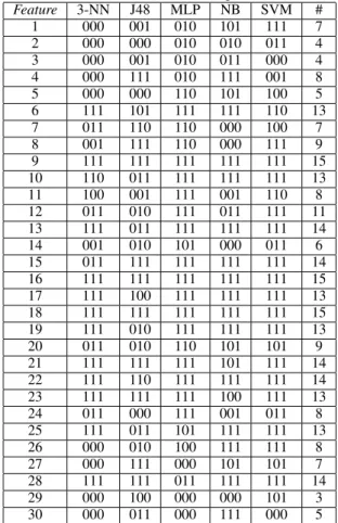
As already mentioned, we also want to analyze if dif-ferent features have the same importance according to their time origin. Table 8 shows a schematic map indicat-ing the features selected in each time segment by our FS procedure. In this table we employ a binary BME mask – for (B)eginning, (M)iddle and (E)nd time segments – where1indicates that the feature was selected in the cor-responding time segment, and0otherwise.

Table 8. Selected features in each time segment (BME mask)

Feature 3-NN J48 MLP NB SVM #

1 000 001 010 101 111 7

2 000 000 010 010 011 4

3 000 001 010 011 000 4

4 000 111 010 111 001 8

5 000 000 110 101 100 5

6 111 101 111 111 110 13

7 011 110 110 000 100 7

8 001 111 110 000 111 9

9 111 111 111 111 111 15

10 110 011 111 111 111 13

11 100 001 111 001 110 8

12 011 010 111 011 111 11

13 111 011 111 111 111 14

14 001 010 101 000 011 6

15 011 111 111 111 111 14

16 111 111 111 111 111 15

17 111 100 111 111 111 13

18 111 111 111 111 111 15

19 111 010 111 111 111 13

20 011 010 110 101 101 9

21 111 111 111 101 111 14

22 111 110 111 111 111 14

23 111 111 111 100 111 13

24 011 000 111 001 011 8

25 111 011 101 111 111 13

26 000 010 100 111 111 8

27 000 111 000 101 101 7

28 111 111 011 111 111 14

29 000 100 000 000 101 3

30 000 011 000 111 000 5

discrimina-tive power of each feature. For example, features 6, 9, 10, 13, 15, 16, 17, 18, 13, 21, 22, 23, 25 and 28 are highly selected, so they are important for music genre classifica-tion. For more discussion, see [31], [33] and [34]. We remember that features 1 to 6 are Beat related, 7 to 25 are related to Timbral Texture, and 26 to 30 are Pitch related.

6. C

In this paper we present a novel approach to the Music Genre Classification Problem, which is based on ensem-ble approach and the decomposition of the music signal according to space and time dimensions. Feature vec-tors are selected from different time segments of the be-ginning, middle and end parts of the music; in order to apply simple but effective classifiers, space decomposi-tion strategies based on the One-Against-All and Round-Robin approaches were used. From the set of partial clas-sification results originated from these views of the prob-lem space, an unique final classification label is provided. A large brand of classical categorization algorithms were employed in the individual segments, and an heuristic combination procedure was used to produce the final mu-sic genre label.

In order to evaluate the proposal we have conducted a extensive set of experiments in a relatively large database – the Latin Music Database, with more than 3,000 mu-sic pieces from 10 mumu-sic genres – specially constructed for this research project. This database was methodically constructed and is open to new research projects in the area.

Several conclusions can be inferred from the obtained results. Firstly, we conclude that the use of the initial 30-second segment of the beginning of the music piece – which is the most frequent strategy used up to now to obtain the music feature vector – is not adequate: our test results show that the middle part is better than the initial or the end parts of the music signal for feature extraction (Table 2). We believe that this phenomena occurs because this middle part the music signal is more stable and more compatible with the corresponding music genre than the others. In fact, results obtained using the middle segment are similar to the ones using the complete music signal; in the latter case, however, the processing time is higher, since there is an obvious relation between the length of the time interval used for feature extraction and the computa-tional complexity of the corresponding extraction proce-dure.

Secondly, we conclude that the use of three time seg-ments and the ensemble of classifiers approach provide better results in accuracy for the AMGC task than the ones obtained from the individual segments (Table 3). This result is in accordance with the conclusions of Li, Ogi-hara and Li [21], who state that specific approaches must be used for labeling different music genres when some

hierarchical classification is considered. So, we believe that our space-time decomposition scheme provides bet-ter classification results. Unfortunately a direct compari-son with the results of Tzanetakis and Cook [35], or the ones of Li, Ogihara and Li [21] is not possible because the GTZAN database provides only the feature values for the initial 30-second segment of the music pieces. Our temporal approach also differs from the one employed by Bergstra et al. [2], that initially uses simple deci-sion stumps applied individually to each feature, and then feature selection and classification in parallel using Ad-aBoost.

In third place we can analyze the results concerning the space decomposition approaches. As already men-tioned, the use of a set of binary classifiers is adequate in problems that present complex class separation surfaces. In general our results show that the RR approach presents superior results regarding the OAA approach (Tables 2 and 3). We justify this fact using the same explanation: in RR individual instances are eliminated – in comparison with the relabeling in the OAA approach – so the con-struction of the separation surface by the classification al-gorithm is simplified. Our best classification accuracy re-sult was obtained with the SVM classifier and space-time decomposition according to the RR approach.

We also evaluate the effect of using a feature selec-tion procedure in the AMGC problem. Our FS procedure is based on the genetic algorithm paradigm. Each indi-vidual works as a mask that selects the set of features to be used for classification. The fitness of the individ-uals is based on the classification performance accord-ing to the wrapper approach. Classical genetic operations (crossover, mutation, elitism) are applied until a stopping criteria is attained.

The results achieved with FS show that this procedure is effective for J48,k-NN and Naïve-Bayes classifiers; for MLP and SVM the FS procedure does not increases clas-sification accuracy (Tables 4, 5, 6 and 7); these results are compatible with the ones presented in [38]. We note that using a reduced set of features implies a smaller pro-cessing time; this is an important issue in practical appli-cations, where a compromise between accuracy and effi-ciency must be achieved.

We also note that the features have different impor-tance in the classification, according to their music seg-ment origin (Table 8). It can be seen, however, that some features are present in almost every selection, showing that they have a strong discriminative power in the classi-fication task.

music signal. Also, our approach represents an interest-ing trade-off between computational effort and classifica-tion accuracy, an important issue in practical applicaclassifica-tions. Indeed, the origin, number and duration of the time seg-ments, the set of discriminative features, and the use of an adequate space decomposition strategy still remain open questions for the AMGC problem.

We intend to improve our proposal in order to increase classification accuracy, by adding a second layer of binary classifiers to deal with classes and/or partial state space views that present higher confusion.

R

[1] J.J. Aucouturier; F. Pachet. Representing musical genre: a state of the art.Journal of New Music Re-search, 32(1):83–93, 2003.

[2] J. Bergstra; N. Casagrande; D. Erhan; D. Eck; B. Kégl. Aggregate features and ADABOOST for mu-sic classification.Machine Learning, 65(2-3):473– 484, 2006.

[3] A. Blum; P. Langley. Selection of relevant features and examples in Machine Learning.Artificial Intel-ligence, 97(1-2):245–271, 1997.

[4] C.H.L. Costa; J. D. Valle Jr; A.L. Koerich. Auto-matic classification of audio data. IEEE Interna-tional Conference on Systems, Man, and Cybernet-ics, pages 562–567, 2004.

[5] A.J.D. Craft; G.A. Wiggins; T. Crawford. How many beans make five? the consensus problem in Music Genre Classification and a new evalu-ation method for single genre categorizevalu-ation sys-tems.Proceedings of the 8th International Confer-ence on Music Information Retrieval, Vienna, Aus-tria, pages 73–76, 2007.

[6] M. Dash; H. Liu. Feature selection for classifi-cation. Intelligent Data Analysis, 1(1-4):131–156, 1997.

[7] T.G. Dietterich. Ensemble methods in Machine Learning. Proceedings of the 1st. International Workshop on Multiple Classifier System, Lecture Notes in Computer Science, 1857:1–15, 2000.

[8] J.S. Downie; S.J. Cunningham. Toward a theory of music information retrieval queries: system design implications.Proceedings of the 3rd International Conference on Music Information Retrieval, pages 299–300, 2002.

[9] J.S. Downie. The Music Information Retrieval Evaluation eXchange (MIREX). D-Lib Magazine, 12(12), 2006.

[10] R. Fiebrink; I. Fujinaga. Feature selection pitfalls and music classification.Proceedings of the 7th In-ternational Conference on Music Information Re-trieval, Victoria, Canada, pages 340–341, 2006.

[11] Y. Freund; R. E. Schapire. A decision-theoretic generalization of on-line learning and an applica-tion to boosting.Journal of Computer and System Sciences, 55(1):119–139, 1997.

[12] J. Fürnkranz. Pairwise Classification as an ensem-ble technique. Proceedings of the 13th European Conference on Machine Learning, Helsinki, Fin-land, pages 97–110, 2002.

[13] M. Grimaldi; P. Cunningham; A. Kokaram. A wavelet packet representation of audio signals for music genre classification using different ensemble and feature selection techniques.Proceedings of the 5th ACM SIGMM International Workshop on Mul-timedia Information Retrieval, ACM Press, pages 102–108, 2003.

[14] M. Grimaldi; P. Cunningham; A. Kokaram. An evaluation of alternative feature selection strate-gies and ensemble techniques for classifying mu-sic. Workshop on Multimedia Discovery and Min-ing, 14th European Conference on Machine Learn-ing, 7th European Conference on Principles and Practice of Knowledge Discovery in Databases, Dubrovnik, Croatia, 2003.

[15] S. Hacker. MP3: The Definitive Guide. O’Reilly Publishers, 2000.

[16] T.K. Ho. Nearest neighbors in random subspaces.

Advances in Pattern Recognition, Joint IAPR Inter-national Workshops SSPR and SPR, Lecture Notes in Computer Science, 1451:640–648, 1998.

[17] J. Kittler; M. Hatef; R.P.W. Duin; and J. Matas. On Combining Classifiers.IEEE Transactions on Pat-tern Analysis and Machine Intelligence, 20(3):226– 239, 1998.

[18] A.L. Koerich; C. Poitevin. Combination of ho-mogenuous classifiers for musical genre classifica-tion. IEEE International Conference on Systems, Man and Cybernetics, IEEE Press, Hawaii, USA, pages 554–559, 2005.

[20] J.H. Lee; J.S. Downie. Survey of music information needs, uses, and seeking behaviours preliminary findings.Proceedings of the 5th International Con-ference on Music Information Retrieval, Barcelona, Spain, pages 441–446, 2004.

[21] T. Li; M. Ogihara; Q. Li. A Comparative study on content-based Music Genre Classification. Pro-ceedings of the 26th Annual International ACM SI-GIR Conference on Research and Development in Informaion Retrieval, Toronto, ACM Press, pages 282–289, 2003.

[22] M. Li; R. Sleep. Genre classification via an LZ78-based string kernel.Proceedings of the 6th Interna-tional Conference on Music Information Retrieval, London, United Kingdom, pages 252–259, 2005.

[23] T. Li; M. Ogihara. Music Genre Classification with taxonomy.Proceedings of IEEE International Con-ference on Acoustics, Speech and Signal Process-ing, Philadelphia, USA, pages 197–200, 2005.

[24] H. Liu; L. Yu. Feature extraction, selection, and construction. The Handbook of Data Mining, Lawrence Erlbaum Publishers, chapter 16, pages 409–424, 2003.

[25] D. McEnnis; C. McKay; I. Fujinaga. Overview of OMEN (On-demand Metadata Extraction Net-work).Proceedings of the International Conference on Music Information Retrieval, Victoria, Canada, pages 7–12, 2006.

[26] D. McEnnis; S.J. Cunningham. Sociology and mu-sic recommendation systems. Proceedings of the 8th International Conference on Music Information Retrieval, Vienna, Austria, pages 185–186, 2007.

[27] A. Meng; P. Ahrendt; J. Larsen. Improving Music Genre Classification by short-time feature integra-tion.Proceedings of the IEEE International Confer-ence on Acoustics, Speech, and Signal Processing, Philadelphia, USA, pages 497–500, 2005.

[28] T. M. Mitchell.Machine Learning. McGraw-Hill, 1997.

[29] L.C. Molina; L. Belanche; A. Nebot. Feature selec-tion algorithms: a survey and experimental evalua-tion.Proceedings of the IEEE International Confer-ence on Data Mining, Maebashi City, Japan, pages 306–313, 2002.

[30] E. Pampalk; A. Rauber; D. Merkl. Content–Based organization and visualization of music archives.

Proceedings of ACM Multimedia, Juan-les-Pins, France, pages 570–579, 2002.

[31] C.N. Silla Jr.; C.A.A. Kaestner; A. L. Koerich. Time-Space ensemble strategies for automatic mu-sic genre classification. Proceedings of the 18th Brazilian Symposium on Artificial Intelligence, Ribeiro Preto, Brazil, Lecture Notes in Computer Science, 4140:339-348, 2006.

[32] C.N. Silla Jr.; C.A.A. Kaestner; A. L. Koerich. The Latin Music Database: a database for the automatic classification of music genres (in portuguese). Pro-ceedings of 11th Brazilian Symposium on Computer Music, So Paulo, BR, pages 167–174, 2007.

[33] C.N. Silla Jr.; C.A.A. Kaestner; A.L. Koerich. Au-tomatic music genre classification using ensemble of classifiers. Proceedings of the IEEE Interna-tional Conference on Systems, Man and Cybernet-ics, Montreal, Canada, pages 1687–1692, 2007.

[34] C. N. Silla Jr.. Classifiers Combination for Auto-matic Music Classification (in portuguese). MSc. Dissertation, Graduate Program in Applied Com-puter Science, Pontifical Catholic University of Paraná, January 2007.

[35] G. Tzanetakis; P. Cook. Musical genre classifica-tion of audio signals.IEEE Transactions on Speech and Audio Processing, 10(5):293–302, 2002.

[36] F. Vignoli. Digital music interaction concepts: a user study. Proceedings of the 5th Interna-tional Conference on Music Information Retrieval, Barcelona, Spain, pages 415-420, 2004.

[37] I. H. Witten; E. Frank. Data Mining: Practical Machine Learning Tools and Techniques. Morgan Kaufmann, 2005.