ISSN 0101-8205 www.scielo.br/cam
An SLP algorithm and its application
to topology optimization*
FRANCISCO A.M. GOMES and THADEU A. SENNE
Departamento de Matemática Aplicada, IMECC
Universidade Estadual de Campinas, 13083-859, Campinas, SP, Brazil
E-mails: chico@ime.unicamp.br / senne@ime.unicamp.br
Abstract. We introduce a globally convergent sequential linear programming method for nonlinear programming. The algorithm is applied to the solution of classic topology optimization
problems, as well as to the design of compliant mechanisms. The numerical results suggest that the
new algorithm is faster than the globally convergent version of the method of moving asymptotes,
a popular method for mechanical engineering applications proposed by Svanberg.
Mathematical subject classification: Primary: 65K05; Secondary: 90C55.
Key words: topology optimization, compliant mechanisms, sequential linear programming, global convergence theory.
1 Introduction
Topology optimization is a computational method originally developed with the aim of finding the stiffest structure that satisfies certain conditions, such as an upper limit for the amount of material. The structure under consideration is under the action of external forces, and must be contained into a design domain . Once the domain is discretized, to each one of its elements we associate a variableχ that is set to 1 if the element belongs to the structure, or 0 if the element is void. Since it is difficult to solve a large nonlinear problem with discrete variables,χis replaced by a continuous variableρ ∈ [0,1], called the element’s “density”.
#CAM-316/10. Received: 15/VIII/10. Accepted: 05/I/11.
However, in the final structure,ρis expected to assume only 0 or 1. In order to eliminate the intermediate values ofρ, Bendsøe [1] introduced theSolid Iso-tropic Material with Penalization method(SIMP for short), which replacesρby the functionρpthat controls the distribution of material. The role of the penalty parameter p>1 is to reduce of the occurrence of intermediate densities.
One of the most successful applications of topology optimization is the design of compliant mechanisms. A compliant mechanism is a structure that is flexible enough to produce a maximum deflection at a certain point and direction, but is also sufficiently stiff as to support a set of external forces. Such mechanisms are used, for example, to build micro-eletrical-mechanical systems (MEMS).
Topology optimization problems are usually converted into nonlinear pro-gramming problems. Since the problems are huge, the iterations of the math-ematical method used in its solution must be cheap. Therefore, methods that require the computation of second derivatives must be avoided. In this paper, we propose a new sequential linear programming algorithm for solving con-strained nonlinear programming problems, and apply this method to the solution of topology optimization problems, including compliant mechanism design.
In the next section, we present the formulation adopted for the basic topology optimization problem, as well as to the compliant mechanism design problem. In Section 3, we introduce a globally convergent sequential linear program-ming algorithm for nonlinear programprogram-ming. We devote Section 4 to our nu-merical experiments. Finally, Section 5 contains the conclusion and suggestions for future work.
2 Problem formulation
The simplest topology optimization problem is the compliance minimization of a structure (e.g. Bendsøe and Kikuchi [2]). The objective is to find the stiffest structure that fits into the domain, satisfies the boundary conditions and has a prescribed volume. After domain discretization, this problem becomes
min
ρ fTu
s.t. K(ρ)u=f
nel X
i=1
viρi ≤V
ρmin≤ρi ≤1, i=1, . . . ,nel,
wherenelis the number of elements of the domain,ρiis the density andvi is the volume of thei-th element,V is the upper limit for the volume of the structure, f is the vector of nodal forces associated to the external loads and K(ρ)is the stiffness matrix of the structure.
When the SIMP model is used to avoid intermediate densities, the global stiffness matrix is given by
K(ρ)= nel
X
i=1 ρipKi,
The parameter ρmin > 0 is used to avoid zero density elements, that would imply in singularity of the stiffness matrix. Thus, forρ ≥ρmin, matrixK(ρ)is invertible, and it is possible to eliminate theuvariables replacingu=K(ρ)−1f in the objective function of problem (1). In this case, the problem reduces to
min
ρ
fT K(ρ)−1f s.t. vTρ ≤V
ρmin≤ρi ≤1, i=1, . . . ,nel,
(2)
This problem has only one linear inequality constraint, besides the box con-straints. However, the objective function is nonlinear, and its computation requires the solution of a linear systems of equations.
2.1 Compliant mechanisms
A more complex optimization problem is the design of a compliant mechanism. Some interesting formulations for this problem were introduced by Nishiwaki et al. [14], Kikuchi et al. [10], Lima [11], Sigmund [16], Pedersen et al. [15], Min and Kim [13], and Luo et al. [12], to cite just a few.
No matter the author, each formulation eventually represents the physical structural problem by means of a nonlinear programming problem. The degree of nonlinearity of the objective function and of the problem constrains vary from one formulation to another. In this work, we adopt the formulation pro-posed by Nishiwaki et al. [14], although similar preliminary results were also obtained for the formulations of Sigmund [16] and Lima [11].
two distinct load cases. In the first case, shown in Figure 1(a), a loadt1is applied to the regionŴt1 ⊂ ∂, and a fictitious loadt2 is applied to a different region Ŵt2 ⊂ ∂, where the deflection is supposed to occur. The optimal structure for this problem is obtained maximizing the mutual energy of the mechanism, subject to the equilibrium and volume constraints. This problem represents the kinematic behavior of the compliant mechanism.
After the mechanism deformation, theŴt2 region eventually contacts a work-piece. In this case, the mechanism must be sufficiently rigid to resist the reac-tion force exerted by the workpiece and to keep its shape. This structural behav-ior of the mechanism is given by the second load case, shown in Figure 1(b). The objective is to minimize the mean compliance, supposing that a load is applied toŴt2, and that there is no deflection at the regionŴt1.
Ω
Γ
dΓ
t1Γ
t2t
t 1
2
Ω
Γ
dΓ
t1Γ
t22 −t
(a) (b)
Figure 1 – The two load cases considered in the formulation of Nishiwaki et al. [14]. These load cases are combined into a single optimization problem. After discretization and variable elimination, this problem becomes
min
ρ
−f T
b K1(ρ)− 1fa fT
c K2(ρ)−1fc s.t. vTρ≤ V
ρmin≤ρi ≤1, i =1, . . . ,nel
This problem has the same constraints of (2). However, the objective func-tion is very nonlinear, and its computafunc-tion requires the solufunc-tion of two linear systems of equations. Other formulations, such as the one proposed by Sig-mund [16], also include constraints on the displacements at certain points of the domain, so the optimization problem becomes larger and more nonlinear.
3 Sequential linear programming
Sequential linear programming (SLP) algorithms have been used successfully in structural design (e.g. Kikuchi et al. [10]; Nishiwaki et al. [14]; Lima [11]; Sigmund [16]). This class of methods is well suited for solving large nonlinear problems due to the fact that it does not require the computation of second derivatives, so the iterations are cheap.
However, for most algorithms actually used to solve topology optimization problems, global convergence results are not fully established. On the other hand, SLP algorithms that are proved to be globally convergent are seldom adopted in practice. In part, this problem is due to the fact that classical SLP algorithms, such as those presented in [21] and [8], have practical drawbacks. Besides, recent algorithms that rely on linear programming also include some sort of tangent step that use second order information (e.g. [5] and [6]).
In this section we describe a new SLP algorithm for the solution of constrained nonlinear programming problems. As it will become clear, our algorithm is not only globally convergent, but can also be easily adapted for solving topology optimization problems.
3.1 Description of the method
Consider the nonlinear programming problem
min f(x) s.t. c(x)=0,
x∈X,
(3)
where the functions f :Rn →Randc :Rn →Rm have Lipschitz continuous first derivatives,
and vectorsxl, xu ∈ Rn define the lower and upper bounds for the
compo-nents of x. One should notice that, using slack variables, any nonlinear pro-gramming problem may be written in the form (3).
The linear approximations for the objective function and for the equality con-straints of (3) in the neighborhood of a pointx∈Rn, are given by
f(x+s) ≈ f(x)+ ∇f(x)Ts≡L(x, s), c(x+s) ≈ c(x)+A(x)s,
whereA(x)=[∇c1(x) . . . ∇cm(x)]T is the Jacobian matrix of the constraints. Therefore, given a point x, we can approximate (3) by the linear program-ming problem
min
s f(x)+ ∇f(x)
Ts s.t. A(x)s+c(x)=0
x+s∈X.
(4)
A sequential linear programming (SLP) algorithm is an iterative method that generates and solves a sequence of linear problems in the form (4). At each iteration k of the algorithm, a previously computed pointx(k) ∈ X is used to generate the linear programming problem. After finding sc, an approximate solution for (4), the variables of the original problem (3) are updated according tox(k+1) =x(k)+sc.
Unfortunately, this scheme has some pitfalls. First, problem (4) may be unlimited even if (3) has an optimal solution. Besides, the linear functions used to define (4) may be poor approximations of the actual functions f and c on a pointx +s that is too far from x. To avoid these difficulties, it is an usual practice to require the step s to satisfy atrust region constraint such as ksk∞ ≤ δ, whereδ > 0, the trust region radius, is updated at each iteration
of the algorithm, to reflect the size of the neighborhood of x where the linear programming problem is a good approximation of (3). Including the trust region in (4), we get the problem
min ∇f(x(k))Ts
s.t. A(x(k))s+c(x(k))=0
sl ≤s≤su
(5)
However, unless x(k) satisfies the constraints of (3), it is still possible that
problem (5) has no feasible solution. In this case, we need not only to improve
f(x(k)+s), but also to find a point that reduces this infeasibility. This can be done, for example, solving the problem
min M(x(k),s)=A(x(k))s+c(x(k))1 s.t. sl
n ≤s≤sun
(6)
where sl
n = max{−0.8δk,xl − x(k)}, sun = min{0.8δk,xu −x(k)}. Clearly, M(x,s) is an approximation for the true measure of the infeasibility given by the function
ϕ(x)= kc(x)k1.
Although the square of the Euclidean norm is the usual choice for defining ϕ(see [9]), due to its differentiability, the one-norm is more appropriate when dealing with an SLP algorithm. Besides avoiding the use of a quadratic function, the one-norm allows the replacement of (6) by the equivalent linear program-ming problem
min Mˉ(x(k),s,z)=eTz
s.t. A(x(k))s+E(x(k))z= −c(x(k))
sln ≤s≤sun z≥0.
(7)
wherez ∈ RmI is a vector of slack variables corresponding to the infeasible constraints, and eT = [1 1. . .1]. To see how matrixE(x(k)) is constructed,
let Ii represent the i-th column of the identity matrix and suppose that {i1,i2, . . . ,imI} are the indices of the nonzero components of c(x
(k)). In this
case, the j-th column ofE(x(k))is given by Ej(x(k))=
(
Iij, ifcij(x(k)) <0,
−Iij, ifcij(x
(k)) >0.
A basic feasible point for (7) can be obtained taking s = 0 and zj = |cij(x(k))|,j =1, . . . ,mI.
prefer to explicitly define a value for this and other parameters of the algo-rithm in order to simplify the notation.
Problems (5) and (6) reveal the two objectives we need to deal with at each iteration of the algorithm: the reduction of f(x)and the reduction ofϕ(x).
If f(x(k) +sc) << f(x(k)) and ϕ(x(k) +sc) << ϕ(x(k)), it is clear that
x(k) +sc is a better approximation than x(k) for the optimal solution of prob-lem (3). However, no straightforward conclusion can be drawn if one of these functions is reduced while the other is increased.
In such situations, we use amerit function to decide ifx(k) can be replaced
byx(k)+sc. In this work, the merit function is defined as
ψ(x, θ )=θf(x)+(1−θ )ϕ(x), (8) whereθ ∈ (0, 1] is a penalty parameter used to balance the roles of f andϕ. The step acceptance is based on the comparison of the actual reduction ofψ with the reduction predicted by the model used to computesc.
The actual reduction ofψ betweenx(k) andx(k)+scis given by Ar ed =θAoptr ed+(1−θ )Ar edf sb,
where
Aoptr ed= f(x(k))− f(x(k)+sc) is the actual reduction of the objective function, and
Ar edf sb =ϕ(x(k))−ϕ(x(k)+sc) is the reduction of the infeasibility.
The predicted reduction of the merit function is defined as
Pr ed =θPr edopt+(1−θ )Pr edf sb,
where
Pr edopt = −∇f(x(k))Tsc is the predicted reduction of f and
Pr edf sb =M(x(k),0)−M(x(k),sc)=c(x(k)) 1−
At the k-th iteration of the algorithm, the step sc is accepted if Ar ed ≥ 0.1Pr ed. If this condition is not verified,δk is reduced and the step is recom-puted. On the other hand, the trust region radius may also be increased if the ratioAr ed/Pr ed is sufficiently large.
The role of the penalty parameter is crucial for the acceptance of the step. Following a suggestion given by Gomes et al. [9], at the beginning of the k-th iteration, we define
θk =min{θ lar ge k , θ
sup
k }, (9)
where
θklar ge =
1+ N
(k+1)1.1
θkmin, (10)
θkmin=min{1, θ0, . . . , θk−1}, (11)
θksup = sup{θ ∈ [0,1] |Pr ed ≥0.5P f sb r ed}
= 0.5 P f sb r ed Pr edf sb−Pr edopt
!
, ifPr edopt ≤ 1 2P
f sb r ed
1, otherwise.
(12)
Whenever the step is rejected,θk is recomputed. However, this parameter is not allowed to increase within the same iteration. The constantN ≥ 0, used to computeθklar ge, can be adjusted to allow a nonmonotone decrease ofθ.
3.2 An SLP algorithm for nonlinear programming
Let us define θ0 = θmax = 1, and k = 0, and suppose that a starting point x(0) ∈ Xand an initial trust region radiusδ
0 ≥ δmin >0 are available. A new SLP method for solving problem (3) is given by Algorithm 1.
In the next subsections we prove that this algorithm is well defined and con-verges to the solution of (3) under mild conditions. In Section 4, we describe a particular implementation of this SLP method for solving the topology opti-mization problem.
3.3 The algorithm is well defined
We say that a point x ∈ Rn is ϕ-stationary if it satisfies the
that satisfies ϕ(x) = 0 is said to be regular if the gradient vectors of the active constraints at x are linearly independent (i.e. the linear independence constraint qualification holds atx).
In this section, we show that, after repeating the steps of Algorithm 1 a finite number of times, a new iteratex(k+1) is obtained. In order to prove this well
definiteness property, we consider three cases. In Lemma 3.1, we suppose that
x(k) is notϕ-stationary and (6) is infeasible. Lemma 3.2 deals with the case in whichx(k) is not ϕ-stationary, but (6) is feasible. Finally, in Lemma 3.3, we suppose thatx(k) is feasible and regular for (3), but does not satisfy the KKT
conditions of this problem.
Lemma 3.1. Suppose thatx(k)is notϕ-stationary and that the condition stated in step 3 of Algorithm 1 is not satisfied. Then after a finite number of step rejections,x(k)+scis accepted.
Proof. Define(s0,z0)=(0, −E(x(k))Tc(x(k)))as the feasible (yet not basic)
initial point for the restoration problem (7), solved at step 2 of Algorithm 1. Define also
dn=(ds, dz)= PN(x(k))(−∇ ˉM(x(k),s0,z0)), (13)
wherePN(x)denotes the orthogonal projection onto the set
N(x)=(s,z)∈Rn+mI|A(x)s+E(x)z= −c(x),
xl−x≤sn≤xu−x, z≥0 . (14)
For a fixed x, Mˉ(x,s,z) is a linear function of s and z. In this case, ∇ ˉM(x,s,z)does not depend on these variables, and we can write ∇ ˉM(x)for simplicity.
Ifx(k)is notϕ-stationary and Mˉ(x(k),sn,z) >0, the reduction of the
infeasi-bility generated bysc≡snsatisfies
Pr edf sb ≥ M(x(k),0)− ˉM(x(k),s0+ ˉαds,z0+ ˉαdz)
= − ˉαeTdz = − ˉα∇ ˉM(x(k))Tdn>0
(15)
where
ˉ
Algorithm 3.1 General SLP algorithm.
1: whilea stopping criterion is not satisfied,do 2: Determinesn, the solution of (7)
3: if Mˉ(x(k),sn,z)=0,then
4: Starting fromsn, determinesc, the solution of (5)
5: else 6: sc←sn.
7: end if
8: Determineθk =min{θklar ge, θksup, θmax} 9: if Ar ed≥0.1Pr edthen
10: x(k+1) ←x(k)+sc 11: if Ar ed≥0.5Pr ed,then
12: δk+1←min{2.5δk,kxu−xlk∞}
13: else
14: δk+1←δmin 15: end if
16: RecomputeA,Eand∇f.
17: θmax←1 18: k ←k+1
19: else
20: δk ←max{0.25ksck∞,0.1δk} 21: θmax←θk
22: end if 23: end while
After rejecting the step and reducingδk a finite number of times, we ev entu-ally getk ˉαdnk∞ = 0.8δk. In this case, definingη = −∇ ˉM(x(k))Tdn/kdnk∞,
we have
Pr edf sb ≥0.8ηδk. (16)
Now, doing a Taylor expansion, we get
c(x(k)+sc)=c(x(k))+A(x(k))sc+O(ksck2), so
Analogously, we have
f(x(k)+sc)=L(x(k),sc)+O(ksck2).
Therefore, forδksufficiently small, Ar ed(δk)= Pr ed(δk)+O(δ2k),so
|Ar ed(δk)−Pr ed(δk)| = O(δk2). (17)
Our choice ofθk ensures thatPr ed≥0.5Pr edf sb. Thus, from (16), we get
Pr ed ≥0.4ηδk. (18)
Finally, from (17) and (18), we obtain
Ar ed(δk) Pr ed(δk)
−1
= O(δk). (19)
Therefore,Ar ed ≥0.1Pr edforδk sufficiently small, and the step is accepted.
Lemma 3.2. Suppose thatx(k)is notϕ-stationary and that the condition stated in step3 of Algorithm 1is satisfied. Then after a finite number of step rejec-tions,x(k)+sc is accepted.
Proof. Letδ(k0)be the trust region radius at the beginning of thek-th iteration, andsabe the solution of
min ksk∞ s.t. As= −c
sln ≤s≤sun. Since x(k) is not ϕ-stationary, ksak
∞ > 0. Now, supposing that the step is
rejected jtimes, we getδk(j) ≤0.25jδk(0). Thus, after
log2 q
0.8δk(0)/ksak∞
attempts to reduceδk,snis rejected and Lemma 3.1 applies.
Lemma 3.3. Suppose that x(k) is feasible and regular for (3), but does not
Proof. Ifx(k) is regular but not stationary for problem (3), then we havedt =
Pϒ(−∇f(x(k)))6=0, where Pϒ denotes the orthogonal projection onto the set
ϒ =s∈Rn | A(x(k))s=0, xl−x(k)≤s≤xu−x(k) . Letαˉ be the solution of the auxiliary problem
min α∇f(x(k))Tdt
s.t. kαdtk∞≤δk α ≥0.
Since this is a linear programming problem, αˉdt belongs to the boundary of the feasible set. Therefore, after reducing δk a finite number of times, we get k ˉαdtk∞=δk, implying thatαˉ =δk/kdtk∞. Moreover,
η= −∇f(x(k))Tdt/kdtk∞>0,
so we have
L(x(k),0)−L(x(k),αˉdt) = − ˉα∇f(x(k))Tdt = − δk
kdtk∞∇ f(x
(k))Tdt =η δ k.
(20)
Combining (20) with the fact thatscis the solution of (5), we get
Pr edopt = L(x(k),0)−L(x(k),sc)
≥ L(x(k),0)−L(x(k),αˉdt)=η δk.
On the other hand, sincex(k)is feasible,
M(x(k),0)= M(x(k),s)=0. Thus,θk =min{1, θ
lar ge
k }is not reduced along withδk, and
Pr ed =θkP opt
r ed ≥θkη δk. (21)
3.4 Every limit point of{x(k)}isϕ-stationary
As we have seen, Algorithm 1 stops when x(k) is a stationary point for prob-lem (3); or whenx(k)isϕ-stationary, but infeasible; or even whenx(k)is feasible but not regular.
We will now investigate what happens when Algorithm 1 generates an infinite sequence of iterates. Our aim is to prove that the limit points of this sequence areϕ-stationary. The results shown below follow the line adopted in [9].
Lemma 3.4. If x∗ ∈ Xis not ϕ-stationary, then there exists ε1, α1, α2 > 0 such that, if Algorithm1is applied tox∈Xandkx−x∗k ≤ε1, then
Pr ed(x)≥min{α1δ, α2}.
Proof. Let (s∗0,z∗0) = (0, −E(x∗)Tc(x∗)) be a feasible initial point and
(s∗n,z∗)be the optimal solution of (7) forx≡x∗.
If x∗ is not ϕ-stationary, there exists ε > 0 such that, for all x ∈ X, kx − x∗k ≤ ε, the constraints that are infeasible at x∗ are also infeasible atx. Thus, for a fixed vector x near x∗, we can consider the auxiliary linear programming problem
min M˜(x,s,z)=eTz
s.t. A(x)s+E(x∗)z= −˜c(x) sln ≤s≤sun
z≥0,
(22)
whereci˜ (x) = ci(x) if ci(x∗) > 0 andci˜ (x) = 0 if ci(x∗) = 0. We denote (˜sn,z˜)the optimal solution of this problem and (s0,z0) = (0, −E(x∗)Tc˜(x)) a feasible initial point.
Following (13), let us define
˜
dn(x)=PN˜(x)(−∇ ˜M(x)),
whereN˜(x)is defined as in (14), usingE(x∗)andc˜(x). One should notice that ˜
dn(x∗)=dn(x∗)=PN(x∗)(−∇ ˉM(x∗)).
Due to the continuity of dn˜ , there must existε1 ∈ (0, ε] such that, for all x∈X,kx−x∗k ≤ε1,
−∇ ˜M(x)Tdn˜ (x)≥ −1 2∇ ˉM(x
and
0<k ˜dn(x)k∞≤2kdn(x∗)k∞.
Now, let us consider two situations. Firstly, suppose that, after solving (22), we get M˜(x,˜sn,z˜) > 0. In this case, ifk ˜dn(x)k∞ ≥ 0.8δ, then from (18) we
have
Pr ed ≥0.4
(−∇ ˜M(x)Tdn˜ (x)) k ˜dn(x)k∞
δ≥0.1(−∇ ˉM(x
∗)Tdn(x∗))
kdn(x∗)k ∞
δ. (23)
On the other hand, if k ˜dn(x)k∞<0.8δ, then from (15) and our choice of θ,
Pr ed ≥ 0.5Pr edf sb≥ −0.5∇ ˜M(x)Tdn˜ (x) ≥ −0.25∇ ˉM(x∗)Tdn(x∗).
(24)
Finally, let us suppose that, after solving (22), we get M˜(x,sn˜ ,z˜) = 0. In this case, Pr edf sb = M˜(x,s0˜ ,z0˜ ), i.e. Pr edf sb is maximum, so (24) also holds. The desired result follows from (23) and (24), for an appropriate choice of
α1andα2.
Lemma 3.5. Suppose thatx∗ is notϕ-stationary and that K1is an infinite set of indices such that limk∈K1x
(k) = x∗. Then {δ
k|k ∈ K1} is bounded away from zero. Moreover, there existα3>0andkˉ >0such that, for k∈ K1, k ≥ ˉk, we have Ar ed≥α3.
Proof. Fork ∈ K1large enough, we havekx−x∗k ≤ε1, whereε1is defined
in Lemma 3.4. In this case, from Lemma 3.1 we deduce that the step is never rejected whenever its norm is smaller than someδ1 > 0. Thus, δk is bounded
away from zero. Moreover, from our step acceptance criterion and Lemma 3.4, we obtain
Ar ed ≥0.1Pr ed≥0.1 min{α1δ1, α2}.
The desired result is achieved choosingα3=0.1 min{α1δ1, α2}.
Hypothesis H1. The sequence{x(k)}generated by Algorithm 1 is bounded.
Theorem 3.1. Suppose that H1holds. If{x(k)}is an infinite sequence gener-ated by Algorithm1, then every limit point of{x(k)}isϕ-stationary.
Proof. To simplify the notation, let us write fk = f(x(k)), ϕk = ϕ(x(k)), ψk =ψ(x(k), θk), andAr ed(k) = Ar ed(x(k),s(ck), θk). From (8), we have that
ψk = θkfk+(1−θk)ϕk− [θk−1fk+(1−θk−1)ϕk] + [θk−1fk+(1−θk−1)ϕk]
= (θk−θk−1)fk−(θk−θk−1)ϕk+θk−1fk+(1−θk−1)ϕk = (θk−θk−1)(fk−ϕk)+ψk−1−A(r edk−1).
Besides, from (9)–(11), we also have that
θk −θk−1≤ N
(k+1)1.1θk−1.
Hypothesis H1 implies that there exists an upper bound c > 0 such that |fk−ϕk| ≤cfor allk∈N, so
ψk ≤ cN
(k+1)1.1θk−1+ψk−1−A
(k−1)
r ed . (25)
Noting thatθk∈ [0,1]for allk, and applying (25) recursively, we get
ψk ≤ k X
j=1 cN
(j+1)1.1 +ψ0− k−1 X
j=0 A(r edj).
Since the series P∞j=1(j+cN1)1.1 is convergent, the inequality above may be
written as
ψk ≤ ˜c− k−1 X
j=0 A(r edj).
Let us now suppose thatx∗∈ Xis a limit point of{x(k)}that is notϕ-stationary. Then, from Lemma 3.5, there existsα3>0 such that Ar ed(k) ≥α3for an infinite set of indices. Besides, A(r edk) >0 for allk. Thus,ψkis unbounded below, which
3.5 The algorithm finds a critical point
In this section, we show that there exists a limit point of the sequence of iter -ates generated by Algorithm 1 that is a stationary point of (3).
Lemma 3.6. For each feasible and regular pointx∗there existsǫ0,σ >ˆ 0such that, whenever Algorithm1 is applied tox ∈ X that satisfieskx−x∗k ≤ ǫ0, we have
ksnk∞≤ kc(x)k1/σ .ˆ and
M(x,0)−M(x,sn(x, δ))≥min{kc(x)k1,σ δ}.ˆ
Proof. Since A(x) is Lipschitz continuous, for each x∗ that is feasible and regular, there existsǫ0such that, for allx ∈ Xsatisfyingkx−x∗k ≤ǫ0,A(x) has full row rank and the auxiliary problem
min Mˉ(x,s,z)=eTz s.t. A(x)s+E(x)z= −c(x)
xl −x≤s≤xu−x z≥0.
(26)
has an optimal solution(s,z)=(ˆs,0). In this case,A(x)ˆs= −c(x), sokˆsk2≤ kc(x)k2/σˆ, whereσ >ˆ 0 is the smallest singular value ofA(x). Since problem (26) is just (7) without the trust region constraintksk∞≤0.8δ, we have
ksnk∞≤ kˆsk∞≤ kˆsk2≤ kc(x)k2/σˆ ≤ kc(x)k1/σ ,ˆ proving the first part of the lemma.
If(ˆs,0)is also feasible for (7), thensn= ˆs, and we have
M(x,0)−M(x,sn(x, δ))= M(x,0)= kc(x)k1. (27) On the other hand, if kˆsk∞ > 0.8δ, then we can define ˆsn = δˆs/kˆsk∞
andznˆ = (1−δ/kˆsk∞)z0(where z0is the z vector corresponding tos = 0),
so (ˆsn,znˆ ) is now feasible for (7). Moreover, since Mˉ(x,0,z0) = kc(x)k1, ˉ
M(x,sˆ,0)=0, andMˉ is a linear function ofsandz, we have M(x,sn(x, δ))= ˉ
M(x,snˆ ,znˆ )=(1−δ/kˆsk∞)kc(x)k1. Thus,
M(x,0)−M(x,sn(x, δ))=δkc(x)k1/kˆsk∞≥ ˆσ δ. (28)
Lemma 3.7. Let {x(k)} be an infinite sequence generated by Algorithm 1.
Suppose that{x(k)}k∈K1 is a subsequence that converges to the feasible and
reg-ular point x∗ that is not stationary for problem (3). Then there exist c1, k1, δ′ >0such that, forx ∈ {x(k)|k ∈ K1, k ≥ k1}, whenever Mˉ(x,sn,z) =0at step3of Algorithm1, we have
L(x,sn)−L(x,sc)≥c1min{δ, δ′}.
Proof. As in Lemma 3.3, let us definedt = PŴ(−∇f(x)), where
Ŵ= {s∈Rn |A(x)s=0, xl ≤x+sn+s≤xu}. Let us also denotesdt the solution of
min L(x,sn+s)= f(x)+ ∇f(x)T(sn+s)
s.t. s=tdt, t ≥0 ksn+sk∞≤δ
xl ≤x+sn+s≤xu
(29)
After some algebra, we note thatsdt = ˜tdt is also the solution of min (∇ f(x)Tdt)t
s.t. 0≤t ≤ ˉt,
where
ˉ
t=min{1, 11, 12},
11=min dti<0
δ+sni
−dti ,
xi +sni −xli −dti
,
12= min dti>0
δ−sni
dti
,xui −xi −sni
dti
.
Since (29) is a linear programming problem and∇ f(x)Tdt <0, we conclude thatt˜= ˉt. Besides,t =1 satisfiesxl ≤x+sn+s≤xu, so
ˉ t=min
1, min
dti<0
δ+sn
i −dti
, min
dti>0
δ−sn
i
dti
. (30)
Remembering thatscis the solution of (5), we obtain
L(sn)−L(sc)≥L(sn)−L(sn+std)= −ˉt∇f(x) T
Since PŴ(−∇f(x)) is a continuous function of x, and x∗ is regular and
feasible but not stationary, there exist c1′, c′2 > 0 and k1 ≥ 0 such that, for allx∈ {x(k)|k ∈ K1, k ≥k1},
kdtk∞≤c′1, (32)
−∇f(x)Tdt ≥c2′. (33)
From (30) and the fact thatksnk∞≤0.8δk, we have that
ˉ t≥min
1, 0.2δ kdtk∞
.
Thus, from (32) we obtain
ˉ t ≥min
1, 0.2δ c′1
= 0.2
c1′ min c′
1
0.2, δ
. (34)
Combining (31), (33) and (34), we get, for allx ∈ {x(k)|k ∈ K1, k≥k0},
L(sn)−L(sc)≥ 0.2c
′
2 c′1 min
c1′
0.2, δ
.
The desired result is obtained takingc1= 0.2c
′
2 c′1 andδ
′ = c ′
1
0.2.
Lemma 3.8. Let{x(k)}be an infinite sequence generated by Algorithm1. Sup-pose that{x(k)}k∈K1 is a subsequence that converges to the feasible and regular
pointx∗ that is not stationary for problem(3). Then there exist β,c2, k2 > 0
such that, wheneverx∈ {x(k)|k ∈ K1, k ≥k2}andkc(x)k1≤βδk, L(x,0)−L(x,sc)≥c2min{δ, δ′}
andθsup(x, δ)=1, whereθsupis given by(12)andδ′is defined in Lemma3.7.
Proof. From Lemma 3.6, we obtain
ksnk∞≤ kc(x)k1/σˆ ≤βδk/σ .ˆ
Therefore, defining β = 0.8σˆ, we get kˆsk∞ ≤ 0.8δk, so Mˉ(x,sn,z) = 0 at
From Lemma 3.7 and the Lipschitz continuity of∇ f(x), we can definek2≥0 such that
L(0)−L(sc) ≥ L(sn)−L(sc)− |L(0)−L(sn)| ≥ c1min{δ, δ′} −O(kc(x)k),
for allx∈ {x(k)|k ∈K1, k≥k2}. Thus, choosingβconveniently, we prove the first statement of the Lemma.
To prove the second part of the lemma, we note that
Pr edf sb =M(0)−M(sc)= M(0)−M(sn)= kc(x)k1,
so
Pr edopt −0.5Pr edf sb ≥c2min{δ, δ′} −0.5kc(x)k1.
Thus, for an appropriate choice ofβ, we obtainPr ed >0.5Pr edf sbforθ =1, and
we get the desired result.
Lemma 3.9. Let{x(k)}be an infinite sequence generated by Algorithm1.
Sup-pose that H1 holds, and that {x(k)}
k∈K1 is a subsequence that converges to
the feasible and regular pointx∗ that is not stationary for problem (3). Then
lim
k→∞θk =0.
Proof. The sequences{θmin
k }and{θ lar ge
k }are bounded below and nonincreas-ing, so both are convergent. Moreover, they converge to the same limit, as limk←∞(θklar ge−θ
min
k ) = 0. Besides, θ min
k+1 ≤ θk ≤ θ lar ge
k . Therefore, {θk} is convergent.
Suppose, for the purpose of obtaining a contradiction, that the infinite se-quence {θk} does not converge to 0. Thus, there must exist k3 ≥ k2 and bθU >bθL >0 such thatbθL ≤θk ≤bθU fork ≥k3.
Now, suppose thatx∈ {x(k)|k ∈ K1, k ≥k3}, andM(x,sn)=0. In this case, from Lemma 3.7, we obtain
Pr ed ≥θ[L(x,0)−L(x,sc)] ≥θc1min{δ, δ′} − O(kc(x)k1).
Sinceθ is not increased if the step is rejected, for eachθtried at the iteration that corresponds tox, we have that
Using a Taylor expansion and the fact that∇f andAare Lipschitz continuous, we obtain
|Ar ed−Pr ed| =O(δ2). (35)
Thus, there existseδ ∈ (0, δ′) ⊂ (0, δmin) such that, if δ ∈ (0,eδ) and x ∈ {x(k)|k ∈ K1, k ≥k3},
|Ar ed−Pr ed| ≤bθLc1eδ/40.
Letk3′ ≥k3be an iteration index such that, for allx∈ {x(k)|k ∈K1, k≥k′3}, and for allθ tried at the iteration that corresponds tox, we have
Pr ed ≥bθLc1min{δ, δ′} −bθLc1eδ/20.
If, in addition,δ∈ [eδ/10,eδ), then
Pr ed ≥bθLc1eδ/20.
Therefore, for allδ ∈ [eδ/10,eδ)and allx∈ {x(k)|k ∈ K1, k ≥k3′}, we have |Ar ed−Pr ed|
Pr ed ≤0.5, (36)
On the other hand, if M(x,sn) > 0, then Pr edopt = 0, so Pr ed = (1−θ )P f sb r ed.
In this case, from (28) and the fact thatθ is not increased if the step is rejected, we get
Pr ed ≥(1−bθU)σ δ.ˆ
Using (35) again, there existseδ ∈ (0, δmin)such that, if δ ∈ (0,eδ)andx ∈ {x(k)|k ∈ K1, k ≥k3},
|Ar ed−Pr ed| ≤(1−bθU)σˆeδ/2,
so (36) also applies.
Thus, for someδ ∈ [eδ/10,eδ), the step is accepted, which means that δk is
bounded away from zero for k ∈ K1, k ≥ k3′, so Pr ed is also bounded away from zero.
Since Ar ed ≥ 0.1Pr ed, the sequence{x(k)} is infinite and the sequence {θk}
is convergent, we conclude that ψ(x, θ ) is unbounded, which contradicts
Lemma 3.10. Let {x(k)} be an infinite sequence generated by Algorithm 1.
Suppose that H1 holds, and that {x(k)}k∈K1 is a subsequence that converges
to the feasible and regular point x∗ that is not stationary for problem (3). If x∈ {x(k)|k ∈ K1, k ≥k2}andkc(x)k1≥βδ, then
δ/θsup=O(kc(x)k1).
Proof. Observe that, whenθsup6=1,
θsup = Pr ed 2(Pr edf sb−Pr edopt)
= M(0)−M(sn)
2[M(0)−M(sn)−L(0)+L(sc)]. From Lemma 3.6, ifx∈ {x(k)|k ∈K1, k≥k2}, we have that
1
2θsup = 1+
L(sc)−L(sn) M(0)−M(sn)+
L(sn)−L(0) M(0)−M(sn)
≤ 1+ |L(0)−L(sn)| M(0)−M(sn)
≤ 1+ O(kc(x)k1) min{kc(x)k1,σ δ}ˆ
≤ 1+ O(kc(x)k1) min{β,σˆ}δ.
Therefore, sincekc(x)k1≥βδ, we haveδ/θsup=O(kc(x)k1).
Lemma 3.11. Let {x(k)} be an infinite sequence generated by Algorithm 1.
Suppose that{x(k)}k∈K1 is a subsequence that converges to the feasible and
reg-ular pointx∗ that is not stationary for problem(3). Then there exist k4 > 0, ˜
θ ∈(0, 1]such that, if
x∈ {x(k)|k ∈ K1, k ≥k4}, kc(x)k1≥βδ and θ ≤ ˜θ satisfies(9)–(12), then Ar ed ≥0.1Pr ed.
Proof. From the fact that∇ f(x)andA(x)are Lipschitz continuous, we may writeAr ed =Pr ed+O(δ2). Now, supposing thatkc(x)k
1≥βδ, we have
Since our choice ofθ ensures that Pr ed ≥ 0.5[M(0)− M(sc)], Lemma 3.6 implies that, fork ∈K1sufficiently large,
Pr ed ≥0.5 min{kc(x)k1,σ δ} ≥ˆ 0.5 min{β,σˆ}δ.
Thus, dividing both sides of (37) by Pr ed, we get
Ar ed Pr ed −1
= O(kc(x)k1),
which yields the desired result.
Lemma 3.12. Let {x(k)} be an infinite sequence generated by Algorithm 1.
Suppose that all of the limit points of {x(k)} are feasible and regular and that
HypothesisH1holds. Then, there exists a limit point of{x(k)}that is a station-ary point of problem(3).
Proof. Following the guidelines of Lemma 13 of [9], we note that, by Hypothesis H1, there exists a convergent subsequence {x(k)}k∈K1. Suppose,
for the purpose of obtaining a contradiction, that the limit point of this sub-sequence is not a stationary point of (3). Then, from Lemma 3.9, we have that limk←∞θk =0.
Since (10)–(11) imply that θklar ge > min{1, θ0, θ1, . . . , θk−1}, there must exist an infinite subsetK2⊂ K1such that
lim k∈K2
θksup(δk)=0, (38)
whereδk is one of the trust region radii tested at iteration k. Therefore, there also existsθ˜,k5>0 such that, for allk ∈ K2,k ≥k5, we haveθklar ge ≤2θkmin,
θksup(δk)≤ ˜θ /2<1, and θk ≤ ˜θ /2. (39) Lemma 3.8 assures that θksup(δ) = 1 for all k ∈ K2 wheneverkc(x(k))k1 ≤ βδ. So, by (38) and (39),
kc(x(k))k1> βδk (40) for allk ∈ K2. Therefore, sincekc(x(k))k1→0, we conclude that
lim k∈K2
Assume, without loss of generality, that
δk ≤0.1δ′<0.1δmin (41)
for allk ∈ K2, whereδ′ is defined in Lemma 3.7. Thus,δk cannot be the first trust region radius tried at iterationk. Let us callδˆk the trust region radius tried
immediately beforeδk, andθˆk the penalty parameter associated to this rejected
step. By (39) and the choice of the penalty parameter, we getθˆk ≤ ˜θ for all k ∈ K2,k ≥ k5. Therefore, Lemma 3.11 applies, sokc(x(k))k1 < βδˆk for all k∈ K2,k ≥k5. Moreover, sinceδk ≥0.1δˆk, inequality (41) implies that
ˆ
δk ≤10δk ≤δ′ < δmin. (42)
Let us define θ′(δˆk) = θklar ge if δˆk was the first trust region radius tested at
iterationk, andθ′(δˆk)=θ (δ′k)otherwise, whereδk′ is the penalty parameter tried
immediately beforeδˆk at iterationk.
From (9)–(12), the fact thatθ is not allowed to increase within an iteration, equation (38) and Lemma 3.8, we have
ˆ
θk = min{θk′(δˆk), θ sup
k (δˆk)} = θk′(δˆk) ≥ min{θ′
k(δˆk), θ sup
k (δk)} = θ sup k (δk)
(43)
for allk ∈ K2,k ≥k5.
Since∇f(x)andA(x)are Lipschitz continuous, we may write |Ar ed(θˆk,δˆk)−Pr ed(θˆk,δˆk)| = O(δˆ2).
for allk ∈ K2,k ≥k5. Besides, by Lemma 3.8, (42) and the definition of Pr ed,
we have
Pr ed(θˆk,δˆk)≥ ˆθkc2δˆk,
so
|Ar ed(θˆk,δˆk)−Pr ed(θˆk,δˆk)| Pr ed(θˆk,δˆk)
= O(δˆ 2) ˆ θkc2δˆk
= O(δ)ˆ ˆ θk
. (44)
From Lemma 3.10 and (40), we obtain
δk/θksup(δk)=O(kc(x(k))k1 for k ∈ K2,k ≥k5.
So, by (42) and (43), we also have δˆk/θ sup
k (δk) = O(kc(x(k))k1. Therefore,
from the feasibility ofx∗, theright-hand side of (44) tends to zero fork ∈ K2, k ≥ k5. This implies that, for k large enough, Ar ed ≥ 0.1Pr ed forδˆk,
Theorem 3.2. Let{x(k)}be an infinite sequence generated by Algorithm1.
Sup-pose that hypotheses H1 andH2 hold. Then all of the limit points of {x(k)} areϕ-stationary. Moreover, if all of these limit points are feasible and regu-lar, there exists a limit point x∗ that is a stationary point of problem (3). In particular, if all of theϕ-stationary points are feasible and regular, there exists a subsequence of{x(k)}that converges to feasible and regular stationary point of(3).
Proof. This result follows from Theorem 3.1 and Lemma 3.12.
4 Computational results
In this section, we present one possible implementation for our SLP algorithm, and discuss its numerical behavior when applied to the solution of some stan-dard topology optimization problems.
4.1 Algorithm details
Steps 2 and 4 constitute the core of Algorithm 1. The implementation of the remaining steps is straightforward.
Step 2 corresponds to the standard phase 1 of the two-phase method for linear programming. If a simplex based linear programming function is available, thensn may be defined as the feasible solution obtained at the end of phase 1, supposing that the algorithm succeeds in finding such a feasible solution. In this case, we can proceed to the second phase of the simplex method and solve the linear programming problem stated at Step 4. One should note, however, that the bounds on the variables defined at Steps 2 and 4 are not the same. Thus, some control over the simplex routine is necessary to ensure that not only the objective function, but also the upper and lower bounds on the variables are changed between phases.
On the other hand, when the constraints given in Step 2 are incompatible, the stepsc is just the solution obtained by the simplex algorithm at the end of phase 1. Therefore, if the two-phase simplex method is used, the computation effort spent at each iteration corresponds to the solution of a single linear pro-gramming problem.
A good alternative is to try to compute Step 4 directly. In case the algorithm fails to obtain a feasible solution, then Steps 2 need to be performed. Fortunately, in the solution of topology optimization, the feasible region of (5) is usually not empty, so this scheme performs well in practice.
4.2 Filtering
It is well known that the direct application of the SIMP method for solving a topology optimization problem may result in a structure containing a check er-board-like material distribution (e.g. Díaz and Sigmund [7]). To circumvent this problem, several regularization schemes were proposed in the literature.
In our experiments, three different schemes were considered, in order to see how they affect the performance of the algorithms. The first one was the den-sity filter proposed by Bruns and Tortorelli [3]. For each elementi, this filter replacesρi by a weighted mean of the densities of the elements belonging to a ballBi with radiusrmax.
Other filter we have tested was the Sinh method of Bruns [4], that combines the density filter with a new scheme for avoiding intermediate densities, re-placing the power function of the SIMP model by the hyperbolic sine function. This filter was chosen because it turns the volume constraint into a nonlinear inequality constraint, so the problem is more difficult to solve.
Finally, we also tried the dilation filter introduced by Sigmund [17]. This filter replaces the density of an element i by the maximum of the densities of the elements that belong to the neighborhood Bi. This filter also turn the volume constraint into a nonlinear constraint, so the related problems are more challenging.
4.3 Description of the tests
In order to confirm the efficiency and robustness of the new algorithm, we com-pare it to the globally convergent version of the Method of Moving Asymptotes, the so called Conservative Convex Separable Approximations algorithm (CCSA for short), proposed by Svanberg [20].
func-tions become greater than or equal to the original funcfunc-tions at the optimal so-lution of the subproblem. A parameter vector, σ, is used to define upper and lower limits for the variables, as well as to convexify the objective and con-straint functions.
We solve four topology optimization problems. The first two are compli-ance minimization problems easily found in the literature: the cantilever and the MBB beams. The last two are compliant mechanism design problems: the gripper and the force inverter. All of them were discretized into 4-node rectan-gular finite elements, using bilinear interpolating functions to approximate the displacements.
We also analyze the effect of the application of the filters presented in Sec-tion 4.2, to reduce the formaSec-tion of checkerboard patterns in the structures. For the density, the dilation and the erosion filters, the penalty parameter p of the SIMP method is set to 1, 2 and 3, consecutively. The Sinh method uses a similar parameter p, that is set to 1 to 6, consecutively.
When the SIMP method is used and p = 1 or 2, the SLP and the CCSA algorithms stop whenever1f, the difference between the objective function of two consecutive iterations, falls below 10−3. For p = 3, both algorithms are halted when1f < 10−3 for three successive iterations. For the sinh method, if p = 1, 2 or 3, we stop the algorithms whenever 1f is smaller than 10−3. If p = 4, 5 or 6, we require that1f < 10−3 for three successive iterations. Besides, for the density filter, we also define a limit of 1000 iterations for each value of the penalty parameter pused by the SIMP method. When the dilation filter is used, this limit is increased to 2800 iterations. For the Sinh filter, a limit of 500 iterations for each pwas adopted. Although not technically sound, this stopping criterion based on the function improvement is quite common in topology optimization.
The initial trust region radius used by the SLP algorithm was set to 0.1. For the CCSA method, the stopping tolerance for the subproblems was set to 10−5. A limit of 20 iterations was also defined for each subproblem. The components of the initial vectorσ0were set to 0.1.
A f
60
30
cm
cm
Figure 2 – Design domain for the cantilever beam.
4.4 Cantilever beam design
The first problem we consider is the cantilever beam presented in Figure 2. We suppose that the structure’s thickness is e = 1cm, the Poisson’s coef fi-cient is σ = 0.3 and the Young’s modulus of the material is E = 1N/cm2. The volume of the optimal structure is limited by 40% of the design domain. A force f = 1N is applied downwards in the center of the right edge of the beam. The domain was discretized into 1800 square elements with 1mm2each. The radius of the filters,rmax, was set to 2.5.
The optimal structures for all of the combinations of methods and filters are shown in Figure 3. Table 1 contains the numerical results obtained, including the optimal value of the objective function, the total number of iterations and the execution time. In this table, the rows labeledRatiocontain the ratio between the values obtained by the SLP and the CCSA algorithms. A ratio marked in bold indicates the superiority of SLP over CCSA.
The cantilever beams shown in Figure 3 are quite similar, suggesting that all of the filters efficiently reduced the formation of checkerboard patterns, as expected. On the other hand, Table 1 shows a clear superiority of the SLP algo-rithm. Although both methods succeeded in obtaining the optimal structure with all of the filters (with minor differences in the objective function values), the CCSA algorithm spent much more time and took more iterations to converge.
4.5 MBB beam design
SLP CCSA
n
o
fi
lte
r
d
e
n
sit
y
d
ilation
S
in
h
Figure 3 – The cantilever beams obtained.
Filter Method Objective Iterations Time (s)
None SLP 75.978 243 51.20
CCSA 77.904 715 212.87
Ratio 0.975 0.34 0.241
Density SLP 72.973 353 95.45
CCSA 72.960 1172 457.85
Ratio 1.000 0.301 0.208
Dilation SLP 73.320 563 650.88
CCSA 73.569 5542 6679.40
Ratio 0.997 0.102 0.097
Sinh SLP 73.784 680 234.52
CCSA 74.297 2317 1796.20
Ratio 0.993 0.293 0.131
cm
A f
150 cm 25
Figure 4 – Design domain for the MBB beam.
coefficient are the same used for the cantilever beam. The volume of the optimal structure is limited by 50% of the design domain. A force f =1N is applied downwards in the center of the top edge of the beam. The radius of the filters,
rmax, was set to 2.5.
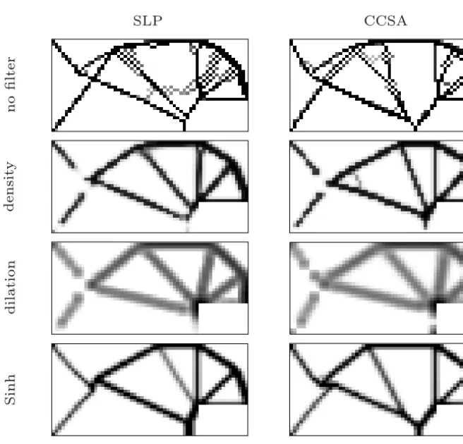
The domain was discretized into 3750 square elements with 1mm2 each. The optimal structures are shown in Figure 5. Due to symmetry, only the right half of the domain is shown. Table 2 contains the numerical results obtained for this problem.
Again, the structures obtained by both methods are similar. The same hap-pens to the values of the objective function, as expected. However, the structure obtained using the density filter has some extra bars. Table 2 shows that the SLP algorithm performs much better than the CCSA method for the MBB beam.
4.6 Gripper mechanism design
Our third problem is the design of a gripper, whose domain is presented in Figure 6. In this compliant mechanism, a force fa is applied to the center of the left side of the domain, and the objective is to generate a pair of forces with magnitude fb at the right side. We consider that the structure’s thickness is e = 1mm, the Young’s modulus of the material is E = 210000N/mm2 and the Poisson’s coefficient is σ = 0.3. The volume of the optimal struc-ture is limited by 20% of the design domain. The input and output forces are fa = fb = 1N. The domain was discretized into 3300 square elements with 1mm2. The filter radius was set to 1.5.
SLP CCSA
n
o
fi
lte
r
d
e
n
sit
y
d
ilation
S
in
h
Figure 5 – The MBB beams obtained.
Filter Method Objective Iterations Time (s)
None SLP 181.524 173 41.29
CCSA 181.020 613 346.57
Ratio 1.003 0.282 0.119
Density SLP 180.618 1054 224.51
CCSA 180.380 2516 2203.50
Ratio 1.001 0.419 0.102
Dilation SLP 185.472 752 896.03
CCSA 185.325 5698 7650.40
Ratio 1.001 0.132 0.117
Sinh SLP 181.453 857 285.487
CCSA 186.601 2694 2620.10
Ratio 0.972 0.318 0.109
A
B
fa
fb 60 mm
15 mm
60 mm 20mm
−fb C
Figure 6 – Design domain for the gripper.
Filter Method Objective Iterations Time (s)
None SLP –5.871 94 46.07
CCSA –7.257 527 2139.50
Ratio 0.809 0.178 0.022
Density SLP –2.924 358 136.30
CCSA –3.669 1302 4034.10
Ratio 0.797 0.275 0.034
Dilation SLP –2.997 847 520.96
CCSA –2.834 2488 12899.00
Ratio 1.057 0.340 0.040
Sinh SLP –1.240 632 255.86
CCSA –1.065 2487 14077.00
Ratio 1.164 0.254 0.018
Table 3 – Results for the gripper mechanism.
SLP CCSA
n
o
fi
lte
r
d
e
n
sit
y
d
ilation
S
in
h
Figure 7 – The grippers obtained.
4.7 Force inverter design
Our last problem is the design of a compliant mechanism known as force inverter. The domain is shown in Figure 8. In this example, an input force
fa is applied to the center of the left side of the domain and the mechanism should generate an output force fbon the right side of the structure. Note that both fa and fb are horizontal, but have opposite directions. For this problem, we also usee = 1mm, σ = 0.3 and E = 210000N/mm2. The volume is limited by 20% of the design domain, and the input and output forces are given by fa = fb = 1N. The domain was discretized into 3600 square elements with 1mm2. The filter radius was set to 2.5.
A
fb B 60 mm
fa 60 mm
Figure 8 – Design domain for the force inverter.
Filter Method Objective Iterations Time (s)
None SLP –4.006 118 46.49
CCSA –4.223 443 485.54
Ratio 0.949 0.266 0.096
Density SLP –1.380 281 131.63
CCSA –1.378 2514 3556.50
Ratio 1.002 0.112 0.037
Dilation SLP –1.084 668 916.84
CCSA –1.014 5741 2679.80
Ratio 1.069 0.116 0.342
Sinh SLP –0.574 512 248.16
CCSA –0.286 820 2019.30
Ratio 2.007 0.624 0.123
Table 4 – Results for the force inverter.
SLP CCSA
n
o
fi
lte
r
d
e
n
sit
y
d
ilation
S
in
h
Figure 9 – The force inverters obtained.
5 Conclusions and future work
filter and trust region radii tested, the Sinh filter presented the best formed structures. Some of the filters allowed the formation of one node hinges. The implementation of hinge elimination strategies, following the suggestions of Silva [18], is one possible extension of this work. We also plan to analyze the behavior of the SLP algorithm in combination with other compliant mecha-nism formulations, such as those proposed by Pedersen et al. [15], Min and Kim [13], and Luo et al. [12].
Acknowledgements. We would like to thank Prof. Svanberg for supplying the source code of his algorithm and Talita for revising the manuscript.
REFERENCES
[1] M.P. Bendsøe,Optimal shape design as a material distribution problem. Struct. Optim.,1(1989), 193–202.
[2] M.P. Bendsøe and N. Kikuchi,Generating optimal topologies in structural design
using a homogenization method. Comput. Methods Appl. Mech. Eng.,71(1988),
197–224.
[3] T.E. Bruns and D.A. Tortorelli,An element removal and reintroduction strategy for
the topology optimization of structures and compliant mechanisms. Int. J. Numer.
Methods Eng.,57(2003), 1413–1430.
[4] T.E. Bruns, A reevaluation of the SIMP method with filtering and an
alterna-tive formulation for solid-void topology optimization. Struct. Multidiscipl. Optim.,
30(2005), 428–436.
[5] R.H. Byrd, N.I.M Gould and J. Nocedal,An active-set algorithm for nonlinear
programming using linear programming and equality constrained subproblems.
Report OTC 2002/4, Optimization Technology Center, Northwestern University, Evanston, IL, USA, (2002).
[6] C.M. Chin and R. Fletcher,On the global convergence of an SLP-filter algorithm
that takes EQP steps. Math. Program.,96(2003), 161–177.
[7] A.R. Díaz and O. Sigmund,Checkerboard patterns in layout optimization. Struct. and Multidiscipl. Optim.,10(1995), 40–45.
[8] R. Fletcher and E. Sainz de la Maza, Nonlinear programming and nonsmooth
optimization by sucessive linear programming. Math. Program.,43(1989), 235–
![Figure 1 – The two load cases considered in the formulation of Nishiwaki et al. [14].](https://thumb-eu.123doks.com/thumbv2/123dok_br/18978192.456059/4.918.182.742.529.827/figure-load-cases-considered-formulation-nishiwaki-et-al.webp)