ISSN 0101-8205 / ISSN 1807-0302 (Online) www.scielo.br/cam
A new double trust regions SQP method
without a penalty function or a filter
∗XIAOJING ZHU∗∗ and DINGGUO PU
Department of Mathematics, Tongji University, Shanghai, 200092, PR China E-mail: [email protected]
Abstract. A new trust-region SQP method for equality constrained optimization is considered. This method avoids using a penalty function or a filter, and yet can be globally convergent to first-order critical points under some reasonable assumptions. Each SQP step is composed of a normal step and a tangential step for which different trust regions are applied in the spirit of Gould and Toint [Math. Program., 122 (2010), pp. 155-196]. Numerical results demonstrate that this new approach is potentially useful.
Mathematical subject classification: 65K05, 90C30, 90C55.
Key words:equality constrained optimization, trust-region, SQP, global convergence.
1 Introduction
We consider nonlinear equality constrained optimization problems of the form
(
min f(x)
s.t. c(x)=0, (1.1)
where we assume that f :Rn
→ Randc : Rn
→ Rm withm
≤ n are twice differentiable functions.
#CAM-414/11. Received: 16/IX/11. Accepted: 22/IX/11.
∗This research is supported by the National Natural Science Foundation of China (No. 10771162).
A new method for first order critical points of problem (1.1) is proposed in this paper. This method belongs to the class of two-phase trust-region methods, e.g., Byrd, Schnabel, and Shultz [3], Dennis, El-Alem, and Maciel [6], Gomes, Maciel, and Martínez [13], Gould and Toint [15], Lalee, Nocedal, and Plantenga [17], Omojokun [21], and Powell and Yuan [23]. Also, our method, since it deals with two steps, can be classified in the area of inexact restoration methods proposed by Martínez, e.g., [1, 2, 8, 18, 19, 20].
The way we compute trial steps is similar to Gould and Toint’s approach [15] that uses different trust regions. Each step is decomposed into a normal step and a tangential step. The normal step is computed by solving a vertical subproblem which aims to minimize the Gauss-Newton approximation of the infeasibility measure within a normal trust region. The tangential step is computed by solving a horizontal subproblem which aims to minimize the quadratic model of the Lagrangian within a tangential trust region on the premise of controlling the linearized infeasibility measure. Similarly, in Martínez’s inexact restoration methods, a more feasible intermediate point is computed in the feasibility phase, and then a trial point is computed on the tangent set that passes through the intermediate point to improve the optimality measure.
Toint’s trust funnel method [15]. These methods adopt the idea of progressively reducing the infeasibility measure. Of course, the new step acceptance mecha-nism in this paper is quite different from the trust funnel and the trust cylinder used in DCI.
The paper is organized as follows. In Section 2, we describe some main details on the new algorithm. Assumptions and global convergence analysis are pre-sented in Section 3. Section 4 is devoted to some numerical results. Conclusions are made in Section 5.
2 The algorithm
2.1 Step computation. At the beginning of this section we define an infeasi-bility measure as follows
h(x), 1 2||c(x)||
2
(2.1)
where|| ∙ ||denotes the Euclidean norm.
Each SQP step is composed of a normal step and a tangential step for which different trust regions are used in the spirit of [15]. The normal step aims to reduce the infeasibility, and the tangential step which approximately lies on the plane tangent to the constraints aims to reduce the objective function as much as possible.
The normal stepnkis computed by solving the trust-region linear least-squares
problem, i.e.,
(
min 12||ck+ Akv||2
s.t. ||v|| ≤1ck.
(2.2)
Here ck = c(xk) and Ak = A(xk) is the Jacobian of c(x) at xk. We do not
require an exact Gauss-Newton step for (2.2), but a Cauchy condition
δkc,n, 1 2||ck||
2
−1
2||ck+Aknk||
2
≥κc||ATkck||min
||AT kck||
1+ ||AT kAk||
, 1ck
(2.3)
for some constantκc ∈(0,1). In addition, we assume the boundedness condition
||nk|| ≤κn||ck|| (2.4)
for some constantκn >0. Note that the above two requirements onnkare very
After obtainingnk, we then aims to find a tangential steptk such that
||t|| ≤1kf (2.5)
to improve the optimality on the premise of controlling the linearized infeasibil-ity measure. Define a quadratic model function
mk(xk+d), fk+ hgk,di +
1
2hd,Bkdi,
where fk = f(xk),gk = ∇f(xk), and Bk is an approximate Hessian of the
Lagrangian
L(x, λ)= f(x)+λTc(x).
Then we have
mk(xk+nk)= fk+ hgk,nki +
1
2hnk,Bknki, and
mk(xk+nk+t) = fk + hgk,nk+ti +
1
2hnk+t,Bk(nk +t)i = mk(xk+nk)+ hgnk,ti +
1
2ht,Bkti, wheregn
k =gk+Bknk.
Let Zk be an orthonormal basis matrix of the null space of Ak if rank(Ak) < n. We assumetk satisfies the following Cauchy-like condition
δkf,t ,mk(xk+nk)−mk(xk+nk+tk)≥κfχkmin
χk
1+ ||Bk||
, 1kf
(2.6)
for some constantκf ∈(0,1), where
χk ,||ZTkg n
k||. (2.7)
Meanwhile we also require tk does not increase the linearized infeasibility
measure too much in the sense that
||ck+Ak(nk+tk)||2≤(1−κt)||ck||2+κt||ck+Aknk||2 (2.8)
for some constant κt ∈ (0,1). This condition on tk can be satisfied if tk is
(2.6) and (2.8) are quite reasonable since we can computetk as a sufficiently
approximate solution to
min hgnk,ti +12ht,Bkti
s.t. Akt=0,
||t|| ≤1kf, which is equivalent to
(
min hZT
kgkn, vi + 1 2hv,Z
T
k BkZkvi
s.t. ||v|| ≤1kf.
The dogleg method or the CG-Steihaug method can therefore be applied [17]. When rank(Ak)=n, we setχk =0 andtk =0.
After obtainingtk, we define the complete step sk =nk+tk.
To obtain a relatively concise convergence analysis, we further impose that
||sk|| ≤1k ,κsmin(1ck, 1 f
k) (2.9)
for some sufficiently large constantκs ≥ 1. In fact, (2.9) can be viewed as an
assumption on the relativity of the sizes of1ckand1kf. It should be made clear thatκc, κf, κn, κt, κs are not chosen by users but theoretical constants. It also
should be emphasized that the double trust regions approach applied here differs from that of Gould and Toint [15]. They do not computetk ifnk lies out of the
ball{v : ||v|| ≤ κBmin(1ck, 1 f
k), κB ∈ (0,1)} and require the complete step sk =nk+tklies within the ball{v: ||v|| ≤min(1ck, 1
f
k)}. In our approach, the
sizes ofnkandtkare more independent of each other, but a stronger assumption
(2.9) is made. For more details about the differences see [15].
Now we consider the estimation of the Lagrange multiplierλk+1. We do not
exactly compute
λk+1= −[ATk] Ig
k,
where the superscriptIdenotes the Moore-Penrose generalized inverse, but
com-puteλk+1approximately solving the least-squares problem
min
λ
1
2||gk+A
T kλ||
such that
||gk+ATkλ|| ≤τ0||gk|| (2.11)
for some toleranceτ0>0.
2.2 Step acceptance. After computing the complete stepsk, we turn to face
with the task of accepting or rejecting the trial pointxk +sk.
We do not use a penalty function or a filter, but establish a new acceptance mechanism to promote global convergence. Let us now construct a dynamic finite set calledh-set,
Hk = {Hk,1,Hk,2,∙ ∙ ∙ ,Hk,l},
where thelelements are sorted in a decreasing order, i.e., Hk,1≥ Hk,2≥ ∙ ∙ ∙ ≥ Hk,l. The h-set is initialized to H0 = {u,∙ ∙ ∙ ,u} for some sufficiently large
constant
u≥max(1,h(x0)), (2.12)
wherex0is the starting point. We then consider the following three conditions:
• h(xk)=0, h(xk+sk)≤ Hk,1; (2.13)
• h(xk) >0, h(xk+sk)≤βh(xk); (2.14)
• h(xk) >0, f(xk+sk)≤ f(xk)−γh(xk+sk),
h(xk+sk)≤βHk,2. (2.15)
Hereβ, γ are two constants such that 0 < γ < β < 1. Note that (2.14) and (2.15) imply
f(xk+sk)≤ f(xk)−γh(xk+sk) or h(xk+sk)≤βh(xk). (2.16)
Afterxk+1= xk+sk has been accepted as the next iterate, we may update the h-set with a new entry
h+k ,(1−θ )h(xk)+θh(xk+1), θ∈(0,1). (2.17)
This means we replace Hk,1withh+k and then re-sort the elements ofh-set in a
is controlled by theh-set, and that the length of theh-setlaffects the strength of infeasibility control although only Hk,1 and Hk,2 are involved in conditions
(2.13-2.15).
All iterations are classified into the following three types:
• f-type. At least one of (2.13-2.15) is satisfied and
χk >0, δkf , f(xk)−mk(xk+sk)≥ζ δkf,t, ζ ∈(0,1). (2.18)
• h-type. At least one of (2.13-2.15) is satisfied but (2.18) fails. • c-type. None of (2.13-2.15) is satisfied.
Ifkis an f-type iteration, we acceptsk and setxk+1=xk+sk if
ρkf , f(xk)− f(xk+sk) δkf ≥
η, η∈(0,1). (2.19)
1kf and1ckare updated according to
1kf+1=
min max(τ11kf,1),ˉ 1ˆ
if ρkf ≥η,
τ21 f
k, if ρ f k < η,
(2.20)
and
1ck+1=
max 1ck,1ˉ if ρkf ≥η,
1ck, if ρkf < η.
(2.21)
Ifk is an h-type iteration, we always acceptsk and setxk+1 = xk +sk. 1 f k
and1ckare updated according to
1kf+1=max(1kf,1),ˉ (2.22)
and
1ck+1=max(1ck,1).ˉ (2.23)
Ifkis ac-type iteration, we acceptsk and setxk+1=xk+skif
δck >0, ρkc, h(xk)−h(xk+sk)
where
δck , 1 2||ck||
2
−12||ck+ Aksk||2.
1ckand1kf are updated according to
1ck+1=
min max(τ11ck,1),ˉ 1ˆ
if ρkc≥η,
τ21ck, if ρ c
k < η, ck 6=0,
1ck, if ρkc< η, ck =0.
(2.25)
and
1kf+1=
max 1kf,1ˉ if ρkc ≥η,
τ21 f
k, if ρ c
k < η, ck =0,
τ21 f
k, if ρ c
k < η, ck 6=0, 1 f k >1,ˉ
1kf, if ρkc < η, ck 6=0, 1kf ≤ ˉ1.
(2.26)
The parameters in (2.20-2.23), (2.25) and (2.26),τ1, τ2,1,ˉ 1, are some positiveˆ
constants such thatτ2<1≤τ1, and1 <ˉ 1.ˆ
One can easily make some conclusions from the update rules of the trust regions. Firstly, we observe that ifkis successful, we have
1kf+1≥ ˉ1 and 1ck+1≥ ˉ1. (2.27)
Secondly,1kf is left unchanged on unsuccessfulc-type iterations whenever xk
is infeasible and 1kf ≤ ˉ1, and1ck is left unchanged on unsuccessful f-type iterations. Thirdly,1kf is reduced on unsuccessful f-type iterations and maybe reduced on unsuccessfulc-type iterations, and 1ck can only be reduced on un-successfulc-type iterations. These properties are very crucial for our algorithm.
2.3 The algorithm. Now a formal statement of the algorithm is presented as follows.
Algorithm 1.A trust-region SQP algorithm without a penalty function or a filter.
Step 0: Initialize k = 0, x0 ∈ Rn, B0 ∈ Sn×n. Choose parameters 1c 0, 1
f 0,
ˉ
1, 1ˆ ∈ (0,+∞) that satisfy 1 < 1ˉ c0, 10f < 1,ˆ β, γ , θ, ζ, η, τ2 ∈
Step 1: Ifk =0 or iterationk−1 is successful, solve (2.10) forλk+1.
Step 2: Solve (2.2) fornk that satisfies (2.3) and (2.4) ifck 6= 0. Setnk = 0
ifck =0.
Step 3: Computetk that satisfies (2.5), (2.6), (2.8) and (2.9) if rank(Ak) <n.
Settk =0 if rank(Ak)=n. Complete the trial stepsk =nk+tk. Step 4: (f-type iteration) One of (2.13-2.15) is satisfied and (2.18) holds.
4.1: Acceptxk+sk if (2.19) holds.
4.2: Update1kf and1ckaccording to (2.20) and (2.21).
Step 5: (h-type iteration) One of (2.13-2.15) is satisfied but (2.18) fails.
5.1: Acceptxk+sk.
5.2: Update1kf and1ckaccording to (2.22) and (2.23).
5.3: Update theh-set withh+k.
Step 6: (c-type iteration) None of (2.13-2.15) is satisfied.
6.1: Acceptxk+sk if (2.24) holds.
6.2: Update1ck and1kf according to (2.25) and (2.26).
6.3: Update theh-set withh+k ifxk+sk is accepted.
Step 7: Accept the trial point. Ifxk+skhas been accepted, setxk+1=xk+sk,
else setxk+1=xk.
Step 8: Update the Hessian. Ifxk+skhas been accepted, choose a symmetric
matrixBk+1.
Step 9: Go to the next iteration. Incrementk by one and go to Step 1.
DCI [1] and the trust-funnel [15], ourh-set mechanism may be more flexible for controlling the infeasibility measure.
3 Global convergence
Before starting our global convergence analysis, we make some assumptions as follows.
Assumptions A
A1. Both f andcare twice differentiable.
A2. There exists a constantκB ≥ 1 such that, ∀ξ ∈ S
k≥0[xk,xk +sk],∀k,
and∀i ∈ {1,∙ ∙ ∙ ,m},
1+max
||gk||,||Bk||,||A(ξ )||,||∇2ci(ξ )||,||∇2f(ξ )|| ≤κB. (3.1) A3. f is bounded below in the level set,
L,
x ∈Rn |h(x)≤u . (3.2)
A4. There exist two constantsκh, κσ >0 such that
h(x)≤κh =⇒ σmin(A(x))≥κσ, (3.3)
whereσmin(A)represents the smallest singular value of A.
In what follows we denote some useful index sets:
S,
k|xk+1=xk+sk
the set of successful iterations, F, H, and C, the sets of f-type,h-type, and
c-type iterations.
The first two lemmas reveal some useful properties of theh-set. These prop-erties play an important role in the following convergence analysis, particularly in driving the infeasibility measure to zero.
Proof. Sincexk is feasible,δkc = 0 and thereforek cannot be a successfulc
-type iteration according to (2.24). Sincexkis a feasible point which is not a first
order critical point, it followsnk =0,δ f k =δ
f,t
k and (2.18) holds. Thusk must
be an f-type iteration. Then, according to the mechanism of the algorithm, each
component ofHkmust be strictly positive.
Lemma 2. For all k, we have
h(xj)≤ Hk,1≤u, ∀ j ≥k, (3.4)
and Hk,1is monotonically decreasing in k.
Proof. Without loss of generality, we can assume that all iterations are suc-cessful. We first prove the following inequality
h(xk)≤ Hk,1 (3.5)
by induction. According to (2.12), we immediately have that (3.5) is true for
k=0. Fork≥1, we consider the following three cases.
The first case is thatk−1∈F. Then one of (2.13-2.15) holds and therefore, according to the hypothesish(xk−1)≤ Hk−1,1, we have from (2.13-2.15) that
h(xk)≤max(Hk−1,1, βh(xk−1), βHk−1,2)=Hk−1,1.
Since theh-set is not updated on an f-type iteration, we have Hk,1 = Hk−1,1.
Thus (3.5) follows.
The second case is thatk−1∈H. Lemma 1 implies thatxk−1is an infeasible
point. Then one of (2.14) and (2.15) holds and Hk−1is updated withh+k−1. It
follows from condition (2.14) or (2.15) that
h(xk)≤βmax(h(xk−1),Hk−1,2).
Therefore the update rules of theh-set, together with (2.17), implies that (3.5) holds.
The third case is thatk−1∈C. Then, according to (2.17) and (2.24), we have
h(xk) <h+k−1. SinceHk−1is updated withh+k−1, it followsh+k−1 ≤ Hk,1. Hence
Since max(h(xk+1),h(xk))≤ Hk,1we haveh+k ≤ Hk,1from (2.17). Thus the
monotonic decrease of Hk,1 follows. Finally, (3.4) follows immediately from
(3.5) and the monotonic decrease ofHk,1.
We now verify that our algorithm satisfies a Cauchy-like condition on the predicted reduction in the infeasibility measure.
Lemma 3. For all k, we have that
δkc≥κtκc||ATkck||min
||ATkck||
1+ ||AT k Ak||
, 1ck
. (3.6)
Proof. It follows from (2.3) and (2.8) that δkc = 1
2||ck||
2
−12||ck +Aksk||2
≥ 12||ck||2−
1
2(1−κt)||ck||
2
− 12κt||ck+Aknk||2
= 12κt(||ck||2− ||ck+Aknk||2)
≥ κtκc||ATkck||min
||AT kck||
1+ ||AT kAk||
, 1ck
.
The following lemma is a direct result of (3.1).
Lemma 4. For all k, we have that
1+ ||ATkAk|| ≤κ2B. (3.7)
Proof. The proof is identical to that of the first part of Lemma 3.1 of [15]. The following lemma is a direct result of Taylor’s theorem.
Lemma 5. For all k, we have that
|f(xk+sk)−mk(xk+sk)| ≤κB||sk||2, (3.8) and
Proof. The proof is similar to that of Lemma 3.4 of [15]. The following lemma is very important as for most of trust-region methods.
Lemma 6. Suppose that k ∈F and that
1kf ≤ (1−η)ζ κfχk κBκs2
. (3.10)
Thenρkf > η. Similarly, suppose that k∈C, ck 6=0, and
1ck ≤ (1−η)κtκc||A
T kck||
κCκs2
. (3.11)
Thenρkc > η.
Proof. The proof of both statements is similar to that of Theorem 6.4.2 of [5]. In fact, using (2.6), (2.18) and (3.1), we have
δkf ≥ζ κfχkmin
χk
1+ ||Bk||
, 1kf
≥ζ κfχkmin
χk
κB
, 1kf
.
Then it follows from (2.9) and (3.8) that if (3.10) holds then
|1−ρkf| =
f(xk+sk)−mk(xk+sk)
δkf
≤ κB||sk||
2
ζ κfχkmin
χk κB, 1
f k
≤ κBκ
2 s(1
f k)
2
ζ κfχk1 f k
≤1−η.
Hence, the first conclusion follows. Similarly, we use (2.9), (3.6), (3.7) and (3.9)
to obtain the second conclusion.
Definiton 1.We callx an infeasible stationary point of hˆ (x)ifx satisfiesˆ A(xˆ)Tc(xˆ)=0 and c(xˆ)6=0.
The algorithm will fail to progress towards the feasible region if started from an infeasible stationary point since no suitable normal step can be found in this situation. If such a point is detected, restarting the whole algorithm from a different point might be the best strategy.
Lemma 7. Suppose that first order critical points and infeasible stationary points never occur. Then we have that|S| = +∞.
Proof. Since xk +sk must be accepted if k is an h-type iteration, we only
consider k ∈ F ∪C. First consider the case that xk is infeasible. Since the
assumption thatxk is not an infeasible stationary point implies||ATkck||>0, it
follows from (3.6) thatδkc >0 and from Lemma 6 thatρkc ≥ ηfor sufficiently small1ck. It also follows from Lemma 6 thatρkf ≥ηfor sufficiently small1kf ifχk >0. Note thatk ∈ F\Simpliesχk > 0,χk+1 =χk, and1
f
k+1 =τ21 f k,
andk ∈ C\Simplies1c
k+1 =τ21ck. Therefore, a successful iteration must be
finished atxkin the end.
Next we consider the case that xk is feasible. Since xk is not a first order
critical point we haveχk >0. Then it follows from Lemma 6 thatρ f
k ≥ ηfor
sufficiently small 1kf. Furthermore, (2.13) must be satisfied if 1kf ≤ q
Hk,1 κC .
Because, according to (3.9) and the fact thatck+Aksk =0 whenck =0 implied
by (2.8), we haveh(xk +sk) ≤ κC||sk||2 ≤ Hk,1. Hence a successful iteration
must be finished atxk in the end.
The following lemma is a crucial result of the mechanism of the algorithm.
Lemma 8. Suppose that, for someǫf >0,
χk ≥ǫf. (3.12)
Then
1kf ≥min μf, τ2
s
Hk,1
κC !
where
μf ,τ2min
(1−η)ζ κfǫf
κBκs2
,1ˉ
.
Moreover, (3.13) can be reduced to 1kf ≥ μf if xk is infeasible. Similarly, suppose that, for someǫc >0,
||ATkck|| ≥ǫc. (3.14)
Then,
1ck ≥μc ,min
τ2(1−η)κtκcǫc
κCκs2
,1ˉ
. (3.15)
Proof. The two statements are proved in the same manner, and immediately result from (2.27), Lemma 6, the proof of Lemma 7 and the update rules of the
the trust-region radii.
Now we consider the global convergence property of our algorithm in the case that successfulc-type andh-type iterations are finitely many.
Lemma 9. Suppose that|S| = +∞and that|(H ∪C)∩S|<+∞. Then
lim
k→∞,k∈Sχk =0, (3.16)
and there exists an infinite subsequenceK⊂Ssuch that
lim
k→∞,k∈Kh(xk)=0. (3.17)
Proof. Since all successful iterations must be f-type for sufficiently largek, we can deduce from (2.18) and (2.19) that f(xk)is monotonically decreasing
ink for all sufficiently largek. For the purpose of deriving a contradiction, we assume that (3.12) holds for an infinite subsequenceK⊂S. Then (2.6), (2.18), (3.1) and (3.13) together yield that, for sufficiently largek ∈K,
δkf ≥ζ κfχkmin
χk
1+ ||Bk||
, 1kf
≥ζ κfǫf min
ǫf
κB
, μf, τ2
s
Hk,1
κC !
Then we have from (2.19) and the above inequality that, for sufficiently large
k∈K,
f(xk)− f(xk+1)≥ηδ f
k ≥ηζ κfǫf min
ǫf
κB
, μf, τ2
s
Hk,1
κC !
.
Since the assumption of the lemma implies that theh-set is updated for finitely many times, we have that Hk,1 is a constant for all sufficiently large k. This,
together with the monotonic decrease of f(xk), implies that limk→∞ f(xk) =
−∞. Since Lemma 2 implies {xk}is contained in the level set Ldefined by
(3.2), the below unboundedness of f(xk)contradicts the assumption A3. Hence
(3.12) is impossible and (3.16) follows.
Now consider (3.17). Assume that xk is infeasible for all sufficiently large k; otherwise (3.17) follows immediately for some infinite subsequenceK⊂S. Then it follows from the monotonic decrease of f(xk), (2.16), and Lemma 1 of
[11] that limk→∞h(xk)=0, which also derives (3.17).
Next we verify that the constraint function must converge to zero in the case thath-type iterations are infinitely many.
Lemma 10. Suppose that|H| = +∞. Thenlimk→∞h(xk)=0.
Proof. DenoteH = {ki}. Recalling that at least one of (2.13-2.15) holds on h-type iterations and thatxki is infeasible by Lemma 1, we deduce from (2.14),
(2.15), (2.17) and (3.4) that
h+k
i = (1−θ )h(xki)+θh(xki+1)
≤ (1−θ )Hki,1+θβmax(Hki,2,h(xki))
≤ (1−θ +θβ)Hki,1.
It then follows from the mechanism of theh-set that
Hki+l,1≤(1−θ+βθ )Hki,1.
Hence, from the above inequality and the monotonic decrease of Hk,1, we have
that
lim
k→∞Hk,1=0. (3.18)
In what follows, to obtain global convergence, we will exclude a scenario for successfulc-type iterations which is less unlikely than being trapped into a local infeasible stationary point. This scenario is
lim
k→∞,k∈C∩S||A T
kck|| =0 with lim inf
k→∞,k∈C∩S||ck||>0. (3.19)
We now verify below that the constraints also converges to zeros in the case that successfulc-type iterations are infinitely many provided that the above undesir-able situation is avoided.
Lemma 11. Suppose that |C ∩S| = +∞and that (3.19)is avoided. Then
limk→∞h(xk)=0.
Proof. We first prove that lim
k→∞,k∈C∩S ||A T
kck|| =0. (3.20)
Assume, for the purpose of deriving a contradiction, that (3.14) holds for some infinite subsequence indexed byK⊂C∩S. Recall that theh-set is updated on successfulc-type iterations and denote{ki} = K. It then follows from (2.17),
(2.24), (3.4), (3.6), (3.7), (3.14) and (3.15) that
Hki,1−h+ki ≥h(xki)−h+ki
=θ (h(xki)−h(xki+1))
≥θ ηδkc
i
≥θ ηκtκc||ATkicki||min
||ATkicki||
1+ ||AT kiAki||
, 1ck
i
!
≥ǫh ,θ ηκtκcǫcmin
ǫc
κ2B, μc
.
It then follows from the above inequality, the monotonic decrease of Hk,1 and
the mechanism of theh-set that
Hki,1−Hki+l,1 ≥ǫh.
This, together with|K| = +∞, yields that Hk,1 is unbounded below, which
Since (3.19) does not hold, it follows from (3.20) that
lim inf
k→∞,k∈C∩S ||ck|| =0.
Thus, there exists an infinite subsequence indexed byJ ⊆C∩Ssuch that
lim
k→∞,k∈J||ck|| =0.
Sinceh(xk+1)≤h(xk)for allk ∈C∩S, the above limit implies
lim
k→∞,k∈Jh + k =0
by (2.17). Then (3.18) follows from the facts that theh-set is updated on suc-cessfulc-type iterations and that Hk,1 is monotonically decreasing. Therefore
the result follows immediately from (3.4) and (3.18).
In what follows, we give the global convergence property of our algorithm in the case that successfulc-type andh-type iterations are infinitely many.
Lemma 12. Suppose that|(H ∪C)∩S| = +∞ and that(3.19)is avoided. Then
lim
k→∞h(xk)=0 (3.21)
and ifβ is sufficiently close to 1, we have
lim inf
k→∞ χk =0. (3.22)
Proof. Limit (3.21) follows immediately from Lemmas 10 and 11. Then we consider (3.22). It follows from (2.4) and (3.21) that
lim
k→∞nk =0. (3.23)
Therefore, from (3.1) and (3.23), we have
lim
k→∞δ f,n
k =0, (3.24)
where
δkf,n, f(xk)−mk(xk +nk)= −gkTnk−
1 2n
Assume now again, for the purpose of deriving a contradiction, that (3.12) holds for allk sufficiently large. Then, if xk is infeasible, we have from (2.6), (3.1),
and Lemma 8 that
δkf,t ≥κfχkmin
χk
1+ ||Bk||
, 1kf
≥ǫt ,κfǫf min
ǫf
κB
, μf
for allk sufficiently large. It then follows from (3.24) that, for all sufficiently largek,
|δkf,n| ≤(1−ζ )ǫt. (3.25)
It is easy to see that, for all sufficiently largeksuch that (3.25) holds, we have δkf
δkf,t =1+ δkf,n
δkf,t ≥1−(1−
ζ )=ζ (3.26)
and therefore (2.18) holds. Ifxk is feasible, thennk = 0 and therefore (2.18)
must hold. Thusk cannot be anh-type iteration for all sufficiently largek. Now consider any sufficiently largek ∈(H ∪C)∩Sso that (3.25) holds and
h(xk)≤κh. (3.27)
Since (3.25) holds, we havek ∈C∩Sby the above analysis. Note that Lemma 1 implies thatxkis infeasible. It follows from (3.3), (3.6), (3.7) and (3.27) that
δkc≥κtκc||ATkck||min
||AkTck||
1+ ||AT k Ak||
, 1ck
≥κtκcκσ||ck||min
κσ||ck||
κ2B , 1
c k
.
(3.28)
Reasoning as in the proof of (3.15) in Lemma 8, one can conclude that
1ck ≥min
τ2(1−η)κtκcκσ||ck||
κCκs2
,1ˉ
.
This, together with limk→∞ck =0, implies that
1ck ≥ τ2(1−η)κtκcκσ||ck|| κCκs2
for all sufficiently largek. Then (3.28) and (3.29) yield δkc≥κtκcκσ||ck||min
κσ||ck||
κ2 B
,τ2(1−η)κtκcκσ||ck|| κCκs2
≥κtκcκσmin
κσ
κ2 B
,τ2(1−η)κtκcκσ κCκs2
||ck||2
≥ τ2(1−η)κ
2 tκ 2 cκ 2 σ
κCκs2
||ck||2
=κβh(xk),
(3.30)
where
κβ ,
2τ2(1−η)κt2κ 2 cκ
2 σ
κCκs2
.
Sincek ∈C∩S, we have from (2.24) and (3.30) that
h(xk+1)≤h(xk)−ηδkc≤(1−ηκβ)h(xk).
Then the above inequality implies that if β ∈ (0,1)is sufficiently close to 1, more specifically, if
1−ηκβ ≤β <1,
it follows
h(xk+1)≤βh(xk).
Then xk+1 satisfies condition (2.14) and therefore k cannot be a c-type
itera-tion, which contradictsk ∈ C. Hence (3.22) holds and the proof is now
com-pleted.
We now present the main theorem on the basis of all the results obtained above.
Theorem 1. Suppose that first order critical points and infeasible stationary points never occur and that(3.19)is avoided. Then there exists a subsequence indexed byKsuch that
lim
k→∞,k∈Kck =0, and ifβ is sufficiently close to 1,
lim
k→∞,k∈KZ T
kgk =0.
Proof. It is easy to see that if lim
k→∞,k∈Kck =0,
then we have from (2.4), (2.7) and (3.1) that
lim
k→∞,k∈Kχk =k→∞lim,k∈KZ T
k(gk+Bknk)= lim k→∞,k∈KZ
T kgk.
This means χk defined by (2.7) is actually an optimality measure for
first-order critical points. Then the desired conclusions immediately follow from
Lemmas 7, 9 and 12.
4 Numerical results
In this section, we present some numerical results for some small size examples to demonstrate our new method may be promising. All the experiments were run in MATLAB R2009b. Details about the implementation are described as follows.
We initialized the approximate Hessian to the identity matrix B0 = I and updated Bk by Powell’s damped BFGS formula [22]. The dogleg method was
applied to compute both normal steps and tangential steps. Moreover, each tangential step was found in the null space of the Jacobian. We computed the Lagrangian multiplier by using MATLAB’s lsqlin function. The parameters for Algorithm 1 were chosen as:
β =0.9999, γ =θ =ζ =η=10−4, τ1=1.1, τ2=0.5, l=3, u =max(500,1.5h(x0)),
1c0=0.5 max(||x0||2,
√
n), 10f =1.21c0, 1ˆ =101c0, 1ˉ =10−4. Now we compare the performance of Algorithm 1 with that of SNOPT Ver-sion 5.3 [12] based on the numbers of function and gradient evaluations required to achieve convergence. A standard stopping criterion is used for Algorithm 1, i.e.,
||ck||∞≤10−6(1+ ||xk||2),
and
The test problems here are all the equality constrained problems from [16]. We ran SNOPT under default options on the NEOS Server (http://www.neos-server.org/neos/solvers/nco:SNOPT/AMPL.html). The corresponding results are shown in Table 1, where Nit, Nf, and Ng represent the numbers of successful iterations, of function evaluations and of gradient evaluations, respectively. It can be observed from Table 1 that Algorithm 1 is generally superior to SNOPT for these problems.
Problem Algorithm 1 SNOPT
Name n m Nit Nf Ng Nit Nf Ng
hs06 2 1 7 8 8 5 9 8
hs07 2 1 10 11 11 18 31 30
hs08 2 2 6 7 7 2 7 6
hs09 2 1 8 9 9 9 9 8
hs26 3 1 19 20 20 25 25 24
hs27 3 1 18 21 19 22 24 23
hs28 3 1 6 7 7 4 4 4
hs39 4 2 18 22 19 20 31 30
hs40 4 3 6 7 7 7 8 7
hs42 4 2 8 9 9 8 9 8
hs46 5 2 29 32 30 28 27 26
hs47 5 3 21 24 22 24 32 31
hs48 5 2 8 12 9 6 6 6
hs49 5 2 22 24 23 37 33 32
hs50 5 3 13 15 14 31 22 21
hs51 5 3 6 8 7 6 6 6
hs52 5 3 8 9 9 5 5 5
hs56 7 4 11 12 12 13 15 14
hs61 3 2 9 10 10 69 169 168
hs77 5 2 11 15 12 15 15 14
hs78 5 3 7 8 8 9 8 7
hs79 5 3 8 11 9 14 15 14
Table 1 – Numerical results.
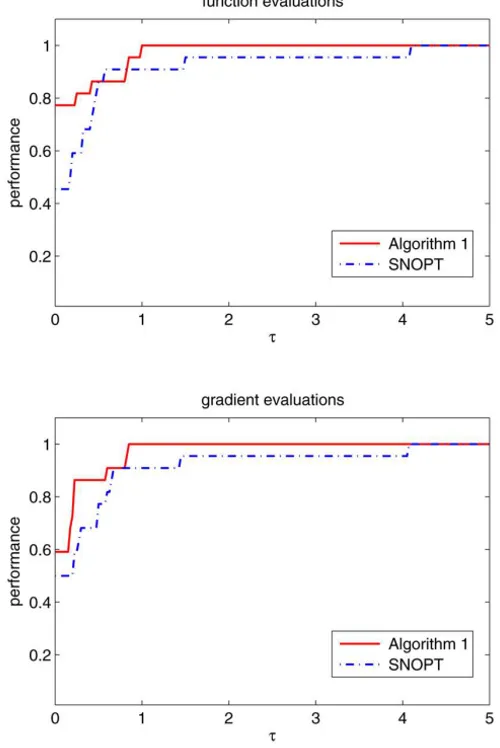
Moré [7] in Figure 1. In the plots, the performance profile is defined by
πs(τ ),
no. of problems where log2(rp,s)≤τ
total no. of problems , τ ≥0,
whererp,sis the ratio of Nf or Ng required to solve problempby solversand the
lowest value of Nf or Ng required by any solver on this problem. The ratiorp,s
is set to infinity whenever solvers fails to solve problem p. It can be observed from Figure 1 that Algorithm 1 outperforms SNOPT for these problems.
5 Conclusions
In this paper, a new double trust regions sequential quadratic programming method for solving equality constrained optimization is presented. Each trial step is computed using a double trust regions strategy in two phases, the first of which aims feasibility and the second, optimality. Thus, the approach is similar to inexact restoration methods for nonlinear programming. The most important feature of this paper is to prove global convergence without using a penalty function or a filter. We propose a new step acceptance technique, the
h-set mechanism, which is quite different from Gould and Toint’s trust-funnel and Bielschowsky and Gomes’ trust cylinder. Numerical results demonstrate the efficiency of this new approach.
REFERENCES
[1] R.H. Bielschowsky and F.A.M. Gomes,Dynamic control of infeasibility in equal-itly constrained optimization.SIAM J. Optim.,19(2008), 1299–1325.
[2] E.G. Birgin and J.M. Martínez, Local convergence of an inexact restoration method and numerical experiments. J. Optim. Theory Appl.,127(2005), 229– 247.
[3] R.H. Byrd, R.B. Schnabel and G.A. Shultz, A trust region algorithm for nonlin-early constrained optimization.SIAM J. Numer. Anal.,24(1987), 1152–1170.
[4] C.M. Chin and R. Fletcher,On the global convergence of an SLP-filter algorithm that takes EQP steps.Math. Program.,96(2003), 161–177.
[5] A.R. Conn, N.I.M. Gould and P.L. Toint, Trust Region Methods, No. 01 in MPS-SIAM Series on Optimization.SIAM, Philadelphia, USA (2000).
[6] J.E. Dennis, M. El-Alem and M.C. Maciel, A global convergence theory for general trust-region-based algorithm for equality constrained optimization.SIAM J. Optim.,7(1997), 177–207.
[7] E.D. Dolan and J.J. Moré,Benchmarking optimization software with performance profiles.Math. Program.,91(2002), 201–213.
[8] A. Fischer and A. Friedlander, A new line search inexact restoration approach for nonlinear programming.Comput. Optim. Appl.,46(2010), 333–346.
[10] R. Fletcher and S. Leyffer, Nonlinear programming without a penalty function.
Math. Program.,91(2002), 239–269.
[11] R. Fletcher, S. Leyffer and P.L. Toint, On the global convergence of a filter-SQP algorithm.SIAM J. Optim.,13(2002), 44–59.
[12] P.E. Gill, W. Murray and M.A. Saunders, SNOPT: an SQP algorithm for large-scale constrained optimization.SIAM Rev.,47(2005), 99–131.
[13] F.M. Gomes, M.C. Maciel and J.M. Martínez, Nonlinear programming algo-rithms using trust regions and augmented lagrangians with nonmonotone penalty parameters.Math. Program.,84(1999), 161–200.
[14] C.C. Gonzaga, E.W. Karas and M. Vanti,A globally convergent filter method for nonlinear programming.SIAM J. Optim.,14(2003), 646–669.
[15] N.I.M. Gould and P.L. Toint, Nolinear programming without a penalty function or a filter.Math. Program.,122(2010), 155–196.
[16] W. Hock and K. Schittkowski, Test examples for nonlinear programming codes, Springer-Verlag (1981).
[17] M. Lalee, J. Nocedal and T.D. Plantenga, On the implementation of an algorithm for large-scale equality constrained optimization.SIAM J. Optim.,8(1998), 682– 706.
[18] J.M. Martínez,Two-phase model algorithm with global convergence for nonlinear programming.J. Optim. Theory Appl.,96(1998), 397–436.
[19] J.M. Martínez, Inexact restoration method with lagriangian tangent decrease and new merit function for nonlinear programming. J. Optim. Theory Appl., 111(2001), 39–58.
[20] J.M. Martínez and E.A. Pilotta, Inexact restoration algorithms for constrained optimization.J. Optim. Theory Appl.,104(2000), 135–163.
[21] E.O. Omojokun,Trust region algorithms for optimization with nonlinear equality and inequality constraints.Ph.D. thesis, Dept. of Computer Science, University of Colorado, Boulder (1989).
[22] M.J.D. Powell,A fast algorithm for nonlinearly constrained optimization calcula-tions.In Numerical Analysis Dundee 1977, G.A. Watson, (ed.), Springer-Verlag, Berlin, (1978), 144–157.
[24] A.A. Ribeiro, E.W. Karas and C.C. Gonzaga, Global convergence of filter methods for nonlinear programming.SIAM J. Optim.,19(2008), 1231–1249.
[25] C. Shen, W. Xue and D. Pu, A filter SQP algorithm without a feasibility restora-tion phase.Comput. Appl. Math.,28(2009), 167–194.
[26] S. Ulbrich, On the superlinear local convergence of a filter-SQP method.Math. Program.,100(2004), 217–245.
[27] A. Wächter and L.T. Biegler, Line search filter methods for nonlinear program-ming: local convergence.SIAM J. Optim.,16(2005), 32–48.