REM WORKING PAPER SERIES
Structural Tax Reforms and Public Spending Efficiency
António Afonso, João Tovar Jalles, Ana Venâncio
REM Working Paper 0146-2020
November 2020
REM – Research in Economics and Mathematics
Rua Miguel Lúpi 20, 1249-078 Lisboa,
Portugal
ISSN 2184-108X
Any opinions expressed are those of the authors and not those of REM. Short, up to two paragraphs can be cited provided that full credit is given to the authors.
REM – Research in Economics and Mathematics
Rua Miguel Lupi, 20 1249-078 LISBOA Portugal Telephone: +351 - 213 925 912 E-mail: [email protected] https://rem.rc.iseg.ulisboa.pt/ https://twitter.com/ResearchRem https://www.linkedin.com/company/researchrem/ https://www.facebook.com/researchrem/
1
Structural Tax Reforms and Public Spending
Efficiency
*
António Afonso
$João Tovar Jalles
#Ana Venâncio
#November 2020
Abstract
We evaluate the effects of structural tax reforms on government spending efficiency in a sample of OECD economies over the period 2007-2016. After calculating input spending efficiency scores, we assess the relevance for efficiency of narrative tax changes in a panel setup. We find that: i) input efficiency scores average around 0.6-07; ii) increases in the tax rates are reflected in falling public sector efficiency; iii) such negative effect is significant for PIT and VAT; iv) controlling for endogeneity, increases in tax rates are still associated with lower public sector efficiency, mainly in PIT; v) increasing tax bases for PIT and VAT improve public sector efficiency; vi) in economic expansion periods, increasing CIT base and reducing PIT rates, positively affect public sector efficiency; ix) in recessions, efficiency improves when PIT and VAT bases increase and CIT rate increases.
JEL: C14, C23, H11, H21, H50
Keywords: government spending efficiency; tax reforms; data envelopment analysis;
non-parametric estimation; panel data; political economy
* The authors acknowledge financial Support from FCT – Fundação para a Ciência e Tecnologia (Portugal), national funding through research grants UIDB/05069/2020 and UIDB/04521/2020. The opinions expressed herein are those of the authors and not necessarily those of their employers.
$ ISEG, Universidade de Lisboa; REM/UECE. Rua Miguel Lupi 20, 1249-078 Lisbon, Portugal. email:
# ISEG, University of Lisbon. REM/UECE. Rua Miguel Lupi 20, 1249-078 Lisbon, Portugal. Economics for Policy and Centre for Globalization and Governance, Nova School of Business and Economics, Rua da Holanda 1, 2775-405 Carcavelos, Portugal. Email: [email protected].
# ISEG, Universidade de Lisboa; ADVANCE/CSG. R. Miguel Lupi 20, 1249-078 Lisbon, Portugal email:
2
1. Introduction
Most countries, through time, have attempted to lift growth by increasing public expenditure, counting that the ensuing income would raise enough revenues to keep the fiscal balance from deteriorating over the long-run. However, several economies have not been able to mobilize revenues through taxation to the same extent as spending went up and, therefore, resorted to internal and external borrowing to finance (growing) deficits. At the same time, according to conventional wisdom, in most countries, larger budget deficits have coincided in the past with less efficient government spending (see, for instance, Afonso et al., 2005).
An interesting avenue of research has linked government spending and public sector efficiency, an issue that has become paramount in a context of scarcer public resources, notably in the aftermath of the 2008-2009 Global Financial Crisis (GFC). Several authors have made efforts to document the degree of government spending inefficiency at the cross-country level but few have tried to explain them. Against this background, a recent paper ty Afonso et al. (2019) reported that expenditure efficiency is usually negatively associated with taxation. More specifically, they found that direct and indirect taxes negatively affected government efficiency performance, and the same being true for social security contributions.
The relevance of tax structures in both developed and developing countries is many fold.1 The distinction and the choice between different types of taxes such as direct vs indirect taxes, for instance, has been an important field of applied research, regarding notably their respective economic growth (un)friendliness.2
In this paper, we contribute to literature by taking a novel view towards the idea that also structural tax reforms, and not necessarily only changes in revenues, can affect the degree of efficiency of the public sector. Tax reforms are needed not only to attain their first objective of raising more revenues, but also secondary objectives such as minimizing their distortionary growth and income distribution effects.3 We explore yet another previously unexplored channel which is whether such reforms help governments offer public services more or less efficiently.
1 Taxation provides resources to the government to perform critical roles such as economic stabilization, allocation and redistribution (Musgrave, 1959). This is particularly relevant in the developing world where collecting more taxes from domestic sources can help achieve the Sustainable Development Goals (SDGs). This is the reason why the Addis Ababa Agenda for financing development pays special attention to domestic resource mobilization in emerging and low-income countries and SDG 17.1 tracks country level domestic resource mobilization efforts. 2 The main channel is that corporate and personal income taxes reduce incentives to raise supply through capital accumulation or productivity enhancements (Schwellnus and Arnold, 2008; Vartia, 2008; Galindo and Pombo, 2011).
3 Common reforms include a shift from trade taxes to domestic sales taxes, the rationalization of income taxes and increase of its progressivity. Another commonly considered policy action includes the shift of the revenue mix away from corporate or personal income tax towards consumption (value-added) and property taxes, which could be growth-enhancing (IMF, 2014).
3
If one observes a decrease in tax revenues, either due to a decline of the tax base or a reduction in a tax rate, and at the end, this can have a direct contractionary effect on the spending side of the government budget. Assuming that the level of public services might still be similar, that would imply an increase in efficiency. Alternatively, an increase in tax revenues through increases in the tax base or rate can increase or not government unnecessary spending.
In this paper we use a new “narrative” database of tax changes put together by Amaglobeli et al. (2018) for a sample of 23 advanced and emerging market economies over the last four decades. We then select all the changes in both tax rates and tax bases of the main tax categories, according to their weight on the total government revenues, namely: personal income taxes (PIT), corporate income taxes (CIT) and value-added taxes (VAT). An important novelty and strength of this database is the precise timing and nature of key legislative tax actions.
Afterwards, we follow a three-step approach. First, we compute composite indicators of government performance. Second, we calculate so-called input efficiency scores for the period 2016-2017. Third, we assess the relevance of the narrative tax changes on the level of the efficiency in a panel setup.
While this new database provides, arguably, an exogenous source for tax reforms, endogeneity can still be a potentially significant concern in our framework since revenue mobilization efforts may not necessarily be exogenous events. We try to address this methodological challenge by controlling for expected economic growth at the time of tax reforms and other possible drivers of government spending efficiency and employing endogeneity robust econometric techniques.
The main findings can be summarized as follows. The average efficiency score throughout the period is around 0.6-07 implying that government spending could be lower by around 30%-40%, on average. We also find a decrease in input efficiency scores around the GFC, and an improvement afterwards.
Regarding the narrative tax base dataset, we observe that countries that increase the tax rates of at least one of the taxes (PIT, CIT or VAT) experience a fall in the level of public sector efficiency. This negative effect seems to operate mainly for PIT and VAT.
Furthermore, controlling for endogeneity, difference-GMM estimations are consistent with previous results: i) increasing tax rate reforms worsens public sector efficiency, mainly due to PIT; ii) increasing tax base reforms improve efficiency, mainly due to PIT and VAT.
Finally, we test if the effect of the tax reforms on public sector efficiency varies across different economic environments, such as recession and expansion. The negative effect of reforms that increase the tax rate occurs mainly in expansion periods, particularly for CIT.
4
Similarly, during expansion periods, reforms that decrease the PIT rate are positively associated with efficiency. In contrast, during recession periods we find opposite effects: CIT rate increases improve efficiency and PIT rate decreases worsens efficiency. In terms of tax base reforms, we find that CIT base increases in expansion periods improves efficiency, while in recessions periods, efficiency worsens if CIT tax base increases and it improves when PIT and VAT tax bases increase.
The remainder of the paper is organized as follows. As background, context and motivation for our empirical analysis, section two provides an overview of related literature. Section three explains the empirical methodology. Section four discusses the empirical results. The last section, concludes and elaborates on policy implications.
2. Literature Review
Previous studies looking specifically to the effectiveness of the public sector (and/or its sub-sectors) have addressed questions such as: are public services satisfactory considering the amount of resources allocated to its activity?; could one have better results using the same amount of resources?; could one obtain the same results with lower expenses?; can one measure cross-country/cross-sector/cross-institution efficiency levels and determine benchmark units?
Afonso and Schuknecht (2019) highlight how governments can improve their overall level of efficiency in terms of the provision of their services, which remains a very topical issue. Indeed, most previous studies reported that government spending efficiency could be enhanced in most OECD countries (see e.g., Afonso et al., 2005, 2010; Afonso and Kazemi, 2018). For instance, Adam et al. (2011), looking at a sample of 19 OECD countries between 1980 and 2000, reported that countries with right-wing and strong governments, high voter participation rates and decentralized fiscal systems, were expected to have more efficient public sectors.
Afonso and Gaspar (2007) illustrated numerically that government financing through distortional taxation causes excess burden (deadweight loss) magnifying the costs of inefficiency. Boadway et al. (1994) rightly mentioned that the tax mix poses several challenges to public finance and can lead to different economic outcomes. Related literature also found that higher taxes typically generate negative consequences for growth by affecting consumption and investment decisions (Feldstein, 2012).4
Earlier theoretical studies on taxation show how higher taxes tend to discourage investment rates (Auerbach and Hasset, 1992) as well as labor supply of individuals (Hausman,
5
1985) and productivity growth. Empirically, a number of studies support the hypothesis that distortive taxes hold back growth more than others (Koester and Kormendi, 1989; Plosser, 1992; Kneller et al., 1999; Gemmell et al., 2011, 2014; Johansson, 2016; Drucker et al., 2017). Corporate and personal income taxes are considered more distortionary than consumption or property taxes as shown by Arnold et al. (2011). Similarly, McNabb and LeMay-Boucher (2014) and Drucker et al. (2017) found that reducing the share of income taxes in the revenue mix would raise GDP growth. Acosta-Ormaechea and Yoo (2019) confirmed that consumption and property taxes are more growth friendly than income taxes. Helms (1985) and Mofidi and Stone (1990) found that taxes revenue spent on publicly provided productive inputs tend to enhance growth. Against this background, Afonso et al. (2019) evaluated to what extent the specificities of a tax system (proxied by revenue-to-GDP ratios) could contribute to government spending efficiency. Other authors used endogenous growth models to simulate the effects of tax reforms on economic growth and found that a decrease in the distorting effects of the current tax structure may lead to a permanent increase in economic growth (Engen and Gale, 1996).
Ultimately, the linkages between the two sides of the government budget, that is, revenue and spending, can convey how fiscal policy is set-up in practice. These are, to great extent, policy decisions since one can typically envisage one-way causality from spending (revenue) to revenue (spending), i.e. “spend-and-tax” (“tax-and-spend” – Friedman, 1978; Chang et al., 2002) causality, two-way causality (fiscal synchronization hypothesis) or no linkages between revenue and spending (von Furstenberg et al., 1986).
The tax-and-spend hypothesis advocates that tax increases will lead to expenditure increases without reducing the budget deficit. Under the spend-and-tax hypothesis, a government’s revenue constraint adjusts to changes in expenditures with some lag. The fiscal synchronization hypothesis suggests that expenditure and revenue decisions are made jointly. Thereby, as advanced by Musgrave (1966), the marginal benefits and the marginal costs of government services are compared by citizens in order to determine the appropriate levels of expenditures and revenues. Payne (1998) found that in most countries the tax-and-spend hypothesis was supported suggesting that any policy to reduce budget deficits via revenues may not result in deficit reduction. On the other hand, Moore and Zanardi (2011) report that central governments in developing countries do not seem to adjust government spending priorities taking into account trade tax revenues-to-GDP ratios, which is would not validate the tax-and-spend hypothesis.
Other studies evaluate the role of individual taxes, such as VAT, as effective tools to reduce central government debt and deficits without increasing government expenditures
6
(Ufier, 2017). Understanding the effect of tax reforms on public sector efficiency has been largely ignored in the literature which is exactly the gap this paper aims to bridge. Interestingly, Barone and Mocetti (2011), using Italian municipalities data, find that taxpayers have a better mood vis-à-vis paying taxes if government revenues are spent in a more efficient fashion.
3. Methodology and Data
3.1. Public Sector Performance and Efficiency Scores
The most commonly used approach to compute the efficiency scores is Data Envelopment Analysis (DEA), which is a non-parametric technique that uses linear programming to compute the production frontier. Formally, for each country i, we have:
𝑌𝑖 = 𝑓(𝑋𝑖), 𝑖 = 1, … , 𝑛 (1)
where𝑌 (Public Sector Performance, PSP) is the composite output measure, and 𝑋 is the input measure, namely Public Expenditure (PE) as a percentage of GDP.
Following the related literature, we use a set of metrics to construct a composite of public sector performance (PSP), as suggested by Afonso et al. (2005, 2019). PSP is the average between opportunity and Musgravian indicators.
The opportunity indicators reflect the governments’ performance in the administration, education, health and infrastructure sectors. The administration sub-indicator includes the following measures: corruption, burden of government regulation (red tape), judiciary independence, shadow economy and the property rights. To measure the education sub-indicator, we use the secondary school enrolment rate, quality of educational system and PISA scores. For the health sub-indicator, we compile data on the infant survival rate, life expectancy and survival rate from cardiovascular diseases (CVD), cancer, diabetes or chronic respiratory diseases (CRD). The infrastructure sub-indicator is measured by the quality of overall infrastructure.
The Musgravian indicators include three sub-indicators: distribution, stability and economic performance. To measure income distribution and inequality, we use the Gini coefficient. For the stability sub-indicator, we use the coefficient of variation for the 5-year average of GDP growth and standard deviation of 5 years inflation. To measure economic performance, we include the 5-year average of GDP per capita, GDP growth and unemployment rate.
7
Accordingly, the opportunity and Musgravian indicators result from the average of the measures included in each sub-indicator. To ensure a convenient benchmark, each sub-indicator measure is first normalized by dividing the value of a specific country by the average of that measure for all the countries in the sample.
Our input measure, Public Expenditure (PE) as a percentage of GDP, weights each area of government expenditure. More specifically, we consider government consumption as input for administrative performance, government expenditure in education as input for education performance, health expenditure as input for health performance and public investment as input for infrastructure performance. For the distribution indicator, we consider expenditures on transfers and subsidies. The stability and economic performance are related to the total expenditure. Table A1 and A2 in Appendix A provide further information on the sources and variable construction.
Returning to Equation (1), inefficiency occurs when 𝑌𝑖 < 𝑓(𝑋𝑖), implying that for an observed level of input, the actual output is smaller than the best attainable output.
To compute the efficiency scores, we adopt an input orientation and assume variable-returns to scale (VRS), to account for the fact that countries might not operate at the optimal scale. The input-oriented approach allows us to evaluate by how much input quantity can be proportionally reduced without changing the output quantities. Alternatively, an output-oriented approach allows us to assess how much output quantities can be proportionally increased without changing the input quantities. The two measures provide the same results under constant returns to scale but give different values under variable returns to scale. Nevertheless, it seems to be more adequate to use an input-oriented setup since the main focus of our analysis relies on decreasing inputs (via both less taxes and less spending).
Formally, we solve the following linear programming problem:
min 𝜃,𝜆 𝜃 𝑠. 𝑡. − 𝑦𝑖 + 𝑌𝜆 ≥ 0 𝜃𝑥𝑖 − 𝑋𝜆 ≥ 0 𝐼1’𝜆 = 1 𝜆 ≥ 0 (2)
where 𝑦𝑖 is a vector of outputs, 𝑥𝑖 is a vector of inputs, 𝜃 is the efficiency scores, 𝜆 is a vector of constants, and 𝐼1’ is a vector of ones.
8
If 𝜃 < 1 , the country is inside the production frontier (i.e., it is inefficient), and if 𝜃 = 1, the country is on the frontier (i.e., it is efficient).
The efficiency scores are computed for all OECD countries5 between the period of 2006 and 2017, except for Mexico. We exclude Mexico because the country is efficient by default, and data heterogeneity is important for the sample analysis.
3.2. Panel Analysis
In the second stage, we empirically assess to what extent structural tax reforms have an impact on the previously computed DEA input efficiency scores. Specifically, we estimate the following reduced-form panel data specification:
𝜃𝑖𝑡 = 𝛽𝑡+ 𝛽𝑖 + 𝑆𝑖𝑡−1′ 𝛽1+ 𝑍𝑖𝑡−1′𝛽2+ 𝜀𝑖𝑡 (3)
where i refers to a given country and t the time period (in years). 𝛽𝑖 denotes country fixed effects to control for unobserved heterogeneity such as geography-specific time invariant characteristics. 𝛽𝑡 denotes time (year) effects to control for global macroeconomic shocks. 𝜀𝑖𝑡 is a disturbance term satisfying standard assumptions of zero mean and constant variance.
Equation (3) is initially estimated using Ordinary Least Squares (OLS) with robust standard errors clustered at the country level. Because time-series cross-sectional data typically display both contemporaneous correlation across units and unit level heteroskedasticity making inference from standard errors produced by OLS incorrect, we also employ Beck and Katz´s (1995) panel-corrected standard error (PCSE) estimator. This estimator is robust to the possibility of non-spherical errors and allow for better inference from linear models estimated in a panel environment. Concerned about autocorrelation of the disturbances, a common AR(1) process is assumed.
Our dependent variable, 𝜃𝑖𝑡, is the DEA input efficient scores, computed in the previous subsection. The input orientation scores flag that higher efficiency is determined by a country’s ability to minimize spending-to GDP ratios by maintaining the same level of public services provision.
5 The 35 OECD countries are: Australia, Austria, Belgium, Canada, Chile, Czech Republic, Denmark, Estonia, Finland, France, Germany, Greece, Hungary, Iceland, Ireland, Israel, Italy, Japan, Korea, Latvia, Lithuania, Luxembourg, the Netherlands, New Zealand, Norway, Poland, Portugal, Slovakia, Slovenia, Spain, Sweden, Switzerland, Turkey, the United Kingdom, and the United States.
9
𝑍𝑖𝑡−1 is a vector of country specific time-varying sociodemographic, macroeconomic and institutional controls that may affect public sector performance. This vector is lagged one year to minimize reverse causality concerns. More specifically, vector 𝑍𝑖𝑡−1 includes: i) a proxy for the country size, defined as the logarithm of domestic residents to control for the monitoring costs of government’s discretional behavior (Grossman et al., 1999); ii) a proxy of economic and technological development given by the logarithm of the number of internet users; iii) a variable related to tourism inflow which might have an impact on the demand of public services (proxied by tourism revenues as share of exports); iv) a measure of fiscal imbalances (proxied by the primary balance and the debt-to-GDP ratio); v) a political dummy identifying if the government´s political ideology is left wing and zero otherwise.
Countries determine the composition of their tax system by making policy changes to tax bases and tax rates. Our key regressors are included in vector 𝑆𝑖𝑡−1, comprising tax reform variables that capture changes (increases or decreases) in both the tax rate and the tax base of three types of taxes (PIT, CIT and VAT).
Data on structural tax reforms come from Amaglobeli et al. (2018) which is now explored carefully in this paper. This dataset covers 23 advanced and emerging market economies.6 From this database, we select all the tax reforms that were implemented between 2005 and 2016. When the year of implementation was not available in the database, we considered the year of announcement. Note that to minimize reverse causality concerns, we evaluate the effect of one-year lag reforms on public sector efficiency. The intersection between this tax reform dataset and the sample of 35 countries for which we have computed input efficiency scores gives a working sample of 18 advanced economies.
Amaglobeli et al. (2018) dataset has several advantages for our own empirical purposes: identifies the precise nature and exact timing of tax actions in key areas of tax policy; identifies the precise tax reforms that underpin what otherwise looks like a gradual improvement in standard tax-to-GDP ratios; identifies reforms that truly led to increases or decreases in revenue, as opposed to just a long list of (small or not economically meaningful) policy changes. The strengths of this “narrative” tax reform database come with one limitation; because two tax reforms in a given area (for example, a change in PIT) can involve different specific actions (for example, rate changes or base changes), only the average impact across historical tax reforms can be estimated. It should be noted that the tax reform database provides no
6The database includes the following countries: Australia, Austria, Brazil, Canada, China, Czech Republic, Denmark, France,
Greece, Germany, India, Ireland, Italy, Japan, Korea, Luxembourg, Mexico, Poland, Portugal, Spain, Turkey, United Kingdom, and the United States.
10
information regarding the current (or past) fiscal stance in the countries under scrutiny, which is not the purpose of this paper.
We focus on the changes in both the tax rates and tax bases of PIT, CIT and VAT. Indeed, in the last year covered in the sample (2017) in the 18 advanced economies, those taxes accounted on average for 54% of total revenues excluding social security and grants (ICTD/UNU-WIDER, 2019). To assess whether upward or downward changes have differentiated effects on the level of the government efficiency, we also discriminate between these two policy measures.
Therefore, we define the following independent variables: a set of dummy variables for changes (increases or decreases) in the base and rate of PIT, CIT and VAT in a specific year. For example, the variable D base increase, t-1, is a dummy variable equal to one if a country increased the tax base of PIT, CIT or VAT in the previous year and zero otherwise.
Table 1 presents stylized facts on tax reforms for PIT, CIT and VAT in our sample of 18 advanced economies between 2005 and 2016, with two 6-year sub-periods. The vast majority of tax revenue reforms in our sample were in the category of PIT, followed by the CIT, and most reforms were implemented during the period 2005-2010. Over the entire period, we also see that there were a larger share of PIT and CIT policy changes towards base and rate decreases, while the reverse was true for VAT.
[Table 1]
Figure 1 provides the number of tax reforms by tax category by country to illustrate the heterogeneity of reform efforts. PIT reforms have been more frequently implemented (close to 50 percent on average across all 18 countries in the sample). In general, fewer major reforms have been implemented in VAT. Some countries were more active in tax reforms that others: on the active side we have countries such as Portugal, Spain and Italy; on the less active side we have countries such as Luxembourg, Czech Republic or the UK.
11
Figure 1. Number of tax reforms by country
(18 advanced economies, 2005-2016)
Source: Authors´ computations.
4. Empirical Results
4.1. Government Efficiency: Stylized Facts
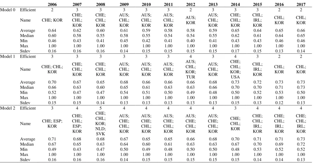
We performed the DEA computations for three models: a baseline model (Model 0), with only one input (PE as percentage of GDP) and one output (PSP); Model 1 with one input, governments’ normalized total spending (PE) and two outputs, the opportunity PSP and the so-called “Musgravian” PSP scores; and Model 2 with two inputs, governments’ normalized spending on opportunity and on “Musgravian” indicators and one output, total PSP scores. The results obtained from these three models are illustrated respectively on Tables B.1, B.2 and B.3 of Appendix B.
Table 2 provides a summary of the DEA results for the three models using an input-oriented assessment. The average efficiency score throughout the period is around 0.6 for the 1 input and 1 output model (Model 0) and around 0.7 in the alternative models (Models 1 and 2). This implies that some possible efficiency gains could be achieved with around less 30% government spending, on average without changing the PSP.
[Table 2]
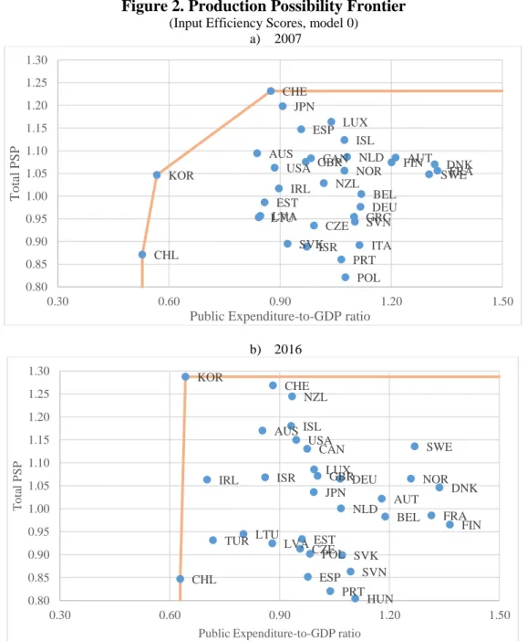
Figure 2 illustrates the production possibility frontier for the baseline model (Model 0), for 2007 (first year of our sample) and for 2016 (last year of our sample), pinpointing notably
0 2 4 6 8 10 12 14 16
12
the countries that define the frontier: Chile, Korea, and Switzerland. For all the other countries inside the frontier, theoretically there would be room for improvement
Figure 2. Production Possibility Frontier
(Input Efficiency Scores, model 0) a) 2007
b) 2016
Note: in the vertical axis we have the total Public Sector Performance (PSP) composite indicator (refer to section 3.1 for details).
Source: Authors´ computations.
Since we are interested in evaluating to what extent the changes in the tax structures impinge on the input efficiency scores throughout time, we report in Figure 3 the development of the input efficiency scores for some countries (for model 2, as an example). Interestingly, we observe some drop in input efficiency scores around the GFC, while afterwards some
AUS AUT BEL CAN CHE CHL CZE DEU DNK ESP EST FIN FRA GBR GRC IRL ISL ISR ITA JPN KOR LTU LUX LVA NLD NOR NZL POL PRT SVK SVN SWE USA 0.80 0.85 0.90 0.95 1.00 1.05 1.10 1.15 1.20 1.25 1.30 0.30 0.60 0.90 1.20 1.50 T o tal P SP
Public Expenditure-to-GDP ratio
AUS AUT BEL CAN CHE CHL CZE DEU DNK ESP EST FIN FRA GBR HUN IRL ISL ISR JPN KOR LTU LUX LVA NLD NOR NZL POL PRT SVK SVN SWE TUR USA 0.80 0.85 0.90 0.95 1.00 1.05 1.10 1.15 1.20 1.25 1.30 0.30 0.60 0.90 1.20 1.50 T o ta l P SP
13
improvement takes place. Here one can think of a possible correlation between the need to implement fiscal consolidations measures in the aftermath of the crisis, notably a decrease in government spending, and the ensuing increase in the measured efficiency scores (plausible if rather the same level of services offered by the government is kept).
Figure 3. Input efficiency scores (model 2)
2a – Australia 2b – Ireland
2c – Poland 2d – Spain
Note: in the vertical axis we report the DEA input efficiency scores using VRS (refer to refer to section 3.1 for details).
Source: Authors´ computations.
4.2. Effects of Structural Tax Reforms on Government Efficiency 4.2.1 Baseline
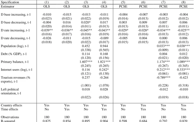
In this sub-section we present the baseline results from estimating Equation (3) using OLS and PCSE methods. This is a reduced-form exercise aimed at quantifying the effects of tax reforms of different types on the degree of public sector efficiency. Although they do not yet directly address endogeneity, these estimates provide a benchmark. Table 3 presents the
14
results using DEA efficiency scores based on Model 2as dependent variable.7 In this table, all three types of tax reforms (PIT, CIT and VAT) are combined into several dummy measures evaluating if a country increased or decreased the tax base or it increased or decreased the tax rate. Specifications (1) and (5) present the estimated results for our key variables of interest including country fixed effects, in specifications (2) and (6) we add year fixed effects, specifications (3) and (7) include the control variables and country fixed effects (without year fixed effects) and specifications (4) and (8) presents the full model.
We observe that countries that increased the tax rate experienced a fall in the level of public sector efficiency. This result is robust to the inclusion of additional controls and using both OLS and PCSE estimators (specifications 3-4 and 7-8). One can consider that higher tax rates (and tax revenues) might feed in into the tax-and-spend causality. Hence, governments might also increase the spending side of their budgets, without necessarily relevant increases in public sector provision.8
As far as other explanatory variables are concerned, we find that an increase on country’s primary balance, possibly through a reduction on public expenditures, and an increase on the level of economic and technological development, measured by the number of internet users, positively and significantly affect efficiency. Consistent with previous literature, public sector efficiency increases with the country’s population but only in the PCSE specifications. This can be seen as evidence of gains via scale economies. Table C.1 in Appendix C, presents our baseline results using alternative DEA-based models, namely Model 0 (one input and one output) and Model 1 (one input and two outputs) as discussed earlier. We continue to find a negative effect of tax rate increases on efficiency in both estimators supporting the tax-and-spend causality. Additionally, we find a positive a significant effect of tax base decreases on efficiency but only in the PCSE specifications.
[Table 3]
Table 4 shows the estimation results disaggregated by tax type using the full model (with control variables and year and country fixed effects) and both estimators. The negative effect of tax rate increases on public sector efficiency seems to operate for all three taxes, however, it is only significant for PIT and VAT (in specifications 1 and 5). Note, however, that these
7 Recall that Model 2 uses two inputs, governments’ normalized spending on opportunity and on “Musgravian” indicators and one output, total PSP scores.
8 The spend-and-tax relationship was addressed, for instance, by Chang et al. (2002) and Kollias and Paleologou (2006).
15
coefficients lose statistical significance when we use the PCSE estimator. We also find that a decrease on the base of VAT is associated with an increase in public sector efficiency for both estimators (OLS and PCSE). Regarding the control variables, we find that population, primary balance and number of internet users continue to positively affect public sector efficiency. The ratio of debt to GDP negatively affects efficiency in the PCSE specifications.
[Table 4]
Next, we conduct several sensitivity and robustness analyses.
4.2.2 Sensitivity and Robustness
We performed sensitivity analysis to inspect if a given country is driving the results. That is, we dropped one country at a time and inspect the stability of the tax reforms effects on public sector efficiency. Figure 4 plots a summary of this exercise with 90 percent confidence intervals for the full model presented in Column 4 of Table 3. We can see that the magnitudes of the tax reforms dummies do not change much, and the negative statistical significance coefficient of tax rate increases also hold for each country.
Figure 4. Sensitivity of tax reform changes to dropping one country at a time
Base increase Base decrease
Rate increase Rate decrease
Source: Authors´ computations. -0.030 -0.020 -0.010 0.000 0.010 0.020 0.030 0.040 0.050 0.060 CI 90% dbaseinc CI 90% -0.030 -0.020 -0.010 0.000 0.010 0.020 0.030 0.040 0.050 CI 90% dbasedec CI 90% -0.080 -0.070 -0.060 -0.050 -0.040 -0.030 -0.020 -0.010 0.000 CI 90% drateinc CI 90% -0.020 -0.010 0.000 0.010 0.020 0.030 0.040 0.050 CI 90% dratedec CI 90%
16
Tax reforms could be implemented because of concerns regarding the future evolution of economic activity. To address this issue, we control for the expected values in t-1 of future real GDP growth. These are taken from the fall issue of the IMF World Economic Outlook for year
t-1. Table C.2 in Appendix C shows the results from adding growth expectations into our baseline
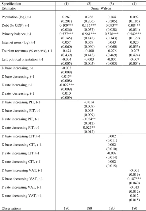
set of controls. We observe that resulting estimates are in line with those presented in Table 3. In addition, equation (3) was re-estimated using Simar and Wilson´s (2007) approach. This method is described by the authors as a superior approach to alternatives such as OLS since this type of naïve estimators ignore that estimated DEA efficiency scores are calculated from a common sample of data and treating them as if they were independent observations is not appropriate.9 Simar and Wilson (2007) procedure takes this (and other pitfalls) into account by constructing an underlying data generating process consistent with two-stage estimation implying a truncated regression model. Table 5 shows the results using the full model and separately for each type of tax reform. Again, countries that implement reforms that increase the tax rate, more specifically in the PIT, experience a reduction of public sector efficiency. Moreover, reforms that decrease the PIT rate are associated with a significant increase on efficiency. We also find a positive and significant effect of reforms that decrease the tax base, mainly on VAT, on public sector efficiency. In terms of control variables, we continue to find a positive and significant effect of the primary balance on public sector efficiency.
[Table 5]
The models that we have been estimating are all reduced-form and therefore do not allow making causal statements or even quantifying the clean effect of tax reforms on public sector efficiency. Adding covariates partly corrects for these biases, but endogeneity can still arise from other omitted variables (unobserved heterogeneity and selection effects), measurement errors in variables, and reverse causality (simultaneity). Because causality can run in both directions, some of the right-hand-side regressors may be correlated with the error term. Preliminary investigation revealed that the dependent variable was serially correlated such that we are required to use a dynamic panel approach to get consistent estimates of Equation (3).
17
Therefore, we employ a dynamic panel estimator, the Generalized Moments Method (GMM) estimator by Arellano & Bond (1991). Dynamic estimators have the following advantages: i) greater control of endogeneity; ii) greater control of possible collinearity between explanatory variables; and iii) greater effectiveness in controlling effects caused by the absence of relevant explanatory variables for the results. GMM estimators are unbiased and compared with OLS or fixed-effects (within-group) estimators, exhibit the smallest bias and variance (Arellano and Bond, 1991). The GMM estimator can only be considered valid if: i) the restrictions, a consequence of use of the instruments, are valid; and ii) there is no second-order autocorrelation.10
Table 6 shows the results for the difference GMM estimator using the full model.11 Consistent with the previous results, we continue to find that countries that implemented reforms that increase the tax rate are associated with a decrease on public sector efficiency. This decrease in efficiency is mainly due to reforms on PIT. Differently from previous estimators, efficiency is positively affected by reforms that increase the tax base. Nonetheless, when we evaluate each type of tax, none of the coefficients is statistically significant. As for the control variables, we find that lag efficiency and primary balance positively and statistically affect public sector efficiency.
[Table 6]
We investigated the stability of GMM results and checked whether the coefficients of interest varied in size, sign and significance with two sets of sensitivity checks. Specifically, we i) dropped non-significant covariates one at a time; and ii) assessed if estimates were sensitive to the choice of lags or the choice of instruments. On the first test, we believe it is preferable to keep insignificant variables in to avoid any possible omitted variable bias, but if the covariates in question do not add information, then their exclusion should not affect the coefficients of the remaining variables. This is exactly what we found when we re-estimated equation (3) by difference-GMM dropping sequentially each of the insignificant covariates. On the second test, lag choice, it is well-known that GMM instrument-generating process can create
10 To test the validity of the restrictions, we use the Hansen test. The null hypothesis indicates that the restrictions imposed by using the instruments are valid. By non rejecting the null hypothesis, we conclude that the restrictions are valid, and the results robust.We test for the existence of first and second-order autocorrelation. The null hypothesis is that there is no autocorrelation. Non rejecting the null hypothesis of non-existence of second-order autocorrelation, we conclude that the results are robust. For the results of the GMM estimator to be considered robust, the restrictions imposed by use of the instruments have to be valid and there can be no second-order autocorrelation.
11 We equally tried estimating Equation (3) with a system GMM estimator and the tenor of the results was very similar to the difference GMM. These results are available on Table C.3 of Appendix C.
18
“too many instruments,” in the sense that some may be “weak” leading to inefficient estimates (Roodman 2009). We re-ran the GMM models with shorter lags (one year, instead of two) and with a shorter set of instruments (in particular, we excluded country-specific time dummies from the instrument set). Here too, the point estimates of the coefficients were not statistically different from the results in Table 6.
A weakness of GMM estimators is that their properties hold when N is large, so they can be severely biased and imprecise in panel data with a small number of cross-sectional units. This is often the case in most macro panels, such as the one employed in this paper. Mindful of this we use the Least Squares Dummy Variable Corrected (LSDC-C) procedure which is based upon the bias approximations derived in Bruno (2005), who extends the result by Kiviet (1999) and Bun and Kiviet (2003) to unbalanced panels. Earlier Monte Carlo studies (Arellano and Bond 1991; Kiviet 1995; Judson and Owen 1999) demonstrate that LSDV, although inconsistent, has a relatively small variance compared to GMM estimators. Hence, LSDV-C emerges as a good alternative estimator for dynamic panel data models with small N and strictly exogenous regressors. That said, one should not forget an important limitation of the procedure: as opposed to GMM estimators, no version of LSDV-C is applicable in the presence of endogenous, or even only weakly exogenous, regressors.
Table 7 shows the results using the full model. We continue to find that reforms associated with tax rate increases negatively affect government efficiency, but the effect is only statistically significant for PIT and VAT. Consistent with OLS, PCSE and Simar-Wilson estimators, we also find that a decrease on the VAT base positively affects efficiency.
[Table 7]
Finally, we explore the role of business cycle conditions in affecting the effect of tax reforms on public sector efficiency. Equation 3 is transformed to allow tax reforms´ effects to vary with the state of the economy, as follows:
𝜃𝑖,𝑡− 𝜃𝑖,𝑡−1 = 𝛽𝑡+ 𝛽𝑖+𝜌𝐿× 𝐹(𝑧𝑖,𝑡)𝑆𝑖,𝑡−1+ 𝜌
𝐻× (1 − 𝐹(𝑧
𝑖,𝑡))𝑆𝑖,𝑡−1+ 𝑍𝑖𝑡−1′𝛽 + 𝜀𝑖𝑡 (4)
with 𝐹(𝑧𝑖𝑡) = exp (−𝛾𝑧𝑖𝑡)
1+exp (−𝛾𝑧𝑖𝑡), 𝛾 > 0, in which 𝑧𝑖𝑡 is an indicator of the state of the economy
(the real GDP growth) normalized to have zero mean and unit variance. The weights assigned to each regime vary between 0 and 1 according to the weighting function 𝐹(. ), so that 𝐹(𝑧𝑖𝑡) can
19
be interpreted as the probability of being in a given state of the economy. The coefficients 𝜌𝐿 and
𝜌𝐻 capture the public sector efficiency impact of tax reforms in cases of extreme recessions
(𝐹(𝑧𝑖𝑡) ≈ 1 when z goes to minus infinity) and booms (1 − 𝐹(𝑧𝑖𝑡) ≈ 1 when z goes to plus infinity), respectively.12 This approach is inspired by the smooth transition autoregressive (STAR) model developed by Granger and Teräsvirta (1993).
Table 8 shows the results of estimating the state contingent equation (4) using difference-GMM estimators. During an expansion period, reforms that increase the tax base positively affect public sector efficiency. Considering the type of taxes, this positive effect is mostly driven by CIT. Efficiency also increases when a country decreases the VAT tax base. Public sector performance also improves when the PIT rate decreases. In contrast, reforms that increase the tax rate negatively affect efficiency, particularly on CIT.
Turning to recession periods, efficiency improves when a country increases the PIT and VAT tax bases and increases the CIT and VAT tax rate. Nevertheless, efficiency diminishes when a country increases the CIT tax base and decreases the PIT tax rate.
[Table 8]
We also considered recessions obtained by applying the Harding and Pagan (2002) algorithm to identify economic turning points and use alternative estimator procedures (PCSE and System-GMM). Results remain qualitatively similar.
5. Conclusion
We have evaluated the effects of structural tax reforms on government spending efficiency in a sample of OECD economies over the period 2007-2016. We begin by computing, via data envelopment analysis, government spending efficiency measures for each country and year in our sample. Then, we empirically assess in a reduced-form regression the relevance of arguably exogenous structural tax reforms on these efficiency measures.
The main findings of our study can be summarized as follows. The average efficiency score throughout the period is around 0.6-07 implying government spending could theoretically be lower by around 30–40%, whilst maintaining the same level of PSP. The countries
12 We choose 𝛾 = 1.5, following Auerbach and Gorodnichenko (2012, 2013), so that the economy spends about 20 percent of the time in a recessionary regime—defined as 𝐹(𝑧𝑖𝑡) > 0.8. Our results hardly change when using
alternative values of the parameter 𝛾, between 1 and 6. Note that 𝐹(𝑧𝑖𝑡)=0.5 is the cutoff between weak and strong
20
delineating the production possibility frontier are Chile, Korea, and Switzerland. In addition, we find a decline in input efficiency scores around the GFC, and an improvement afterwards.
We observe that countries that increased the tax rates of at least one of the taxes (PIT, CIT or VAT) experience a fall in the level of public sector efficiency. Indeed, governments might increase also the spending side of their budgets, without necessarily relevant increases in public sector provision. The negative effect of an increase of tax rates on public sector efficiency seems to operate mainly on PIT and VAT.
Accounting for endogeneity, the results of the difference-GMM estimations are consistent with the previous results: i) reforms that increase the tax rate are associated with a decrease on public sector efficiency, mainly due through PIT; ii) reforms that increase the tax base for positively affect public sector efficiency, mainly due to PIT and VAT.
Finally, we test if the effect of the tax reforms on public sector efficiency varies across different economic environments, such as recession and expansion. The negative effect of reforms that increase the tax rate occurs mainly in expansion periods, particularly for CIT. Similarly, during expansion periods, reforms that decrease the PIT rate are positively associated with efficiency. In contrast, during recession periods we find opposite effects: CIT rate increases improve efficiency and PIT rate decreases worsens efficiency. In terms of tax base reforms, we find that CIT base increases in expansion periods improves efficiency, while in recessions periods, efficiency worsens if CIT base increases and it improves when PIT and VAT bases increase.
Our results leave some questions open for future research. Perhaps most importantly, cross-country public sector efficiency differences go way beyond the tax reform areas covered in this paper and include, among others, reforms in areas such as pension, unemployment insurance schemes and healthcare systems. A more systematic investigation of their aggregate effects on public sector efficiency would, therefore, be welcomed. In addition, the effect of tax reforms on efficiency outcomes is likely to vary across countries depending on their specific structural characteristics, particularly those of a political economy nature.13 Further investigating these could shed light on the extent and underlying drivers of cross-country heterogeneity in the government efficiency impacts of reforms more generally. Lastly, this paper did not elaborate on tax efficiency considerations nor did it look at whether the tax composition resulting from tax reforms was optimal from a welfare point of view. This could also be an avenue of future research.
13 Political barriers are in part responsible for a reliance on narrow technocratic reforms which are being ineffective at raising more revenues.
21
References
1. Acosta-Ormaechea, S., Sola, S., Yoo, J. (2019). “Tax composition and growth: A broad cross-country perspective” German Economic Review, 20(4), 70-106
2. Adam, A., Delis, M., Kammas, P. (2011). “Public sector efficiency: levelling the playing field between OECD countries”, Public Choice, 146 (1-2), 163–183.
3. Afonso, A., Alves, J. (2019). “Tax Structure for Consumption and Income Inequality: an Empirical Assessment”, SERIEs - Journal of the Spanish Economic Association, 10 (3-4), 337-364.
4. Afonso, A., Gaspar, V. (2007). “Dupuit, Pigou and cost of inefficiency in public services provision”, Public Choice, 132 (3-4), 485-502.
5. Afonso, A., Jalles, J., Venâncio, A. (2019). “Taxation and Public Spending Efficiency: An International Comparison”, REM WP 080-119.
6. Afonso, A., Kazemi, M. (2017). “Assessing Public Spending Efficiency in 20 OECD Countries”, in Inequality and Finance in Macrodynamics (Dynamic Modelling and
Econometrics in Economics and Finance), Bökemeier, B., Greiner, A. (Eds). Springer.
7. Afonso, A., Schuknecht, L., Tanzi, V. (2005). “Public Sector Efficiency: An International Comparison”, Public Choice, 123 (3-4), 321-347.
8. Afonso, A., Schuknecht, L., Tanzi, V. (2010). “Public Sector Efficiency: Evidence for New EU Member States and Emerging Markets”, Applied Economics, 42 (17), 2147-2164. 9. Amaglobeli, D., Crispolti, V., Dabla-Norris, E., Karnane, P., Misch. F. (2018). “Tax Policy
Measures in Advanced and Emerging Economies: A Novel Database”, IMF WP 18/110. 10. Arnold, J., Brys, B., Heady, C., Johansson, A., Schwellnus, C., Vartia L. (2011). “Tax
Policy for Economic Recovery and Growth,” Economic Journal, 121 (550), 59–80.
11. Auerbach, A., Gorodnichenko. Y. (2012). “Output Spillovers from Fiscal Policy”. NBER working Paper #18578.
12. Auerbach, A., Gorodnichenko. Y. (2013). “Fiscal Multipliers in Recession and Expansion”, in Fiscal Policy after the Financial Crisis, A. Alesina and F. Giavazzi, eds., University of Chicago Press.
13. Auerbach, A.J., Hassett, K. (1992). “Tax Policy and Business Fixed Investment," Journal
of Public Economics, 47, 141-170.
14. Barone, G., Mocetti, S. (2011). “Tax morale and public spending inefficiency”,
International Tax and Public Finance, 18 (6), 724-749.
15. Boadway, R., Marchand, M., Pestieau, P. (1994). “Towards a theory of the direct-indirect tax mix” Journal of Public Economics, 55 (1), 71-88.
22
16. Bruno, G. (2005). “Approximating the bias of the LSDV estimator for dynamic unbalanced panel data models,” Economics Letters, 87(3), 361–366.
17. Bun, M.J.G., Kiviet, J.F. (2003). “On the diminishing returns of higher order terms in asymptotic expansions of bias”. Economics Letters, 79, 145-152.
18. Chang, T.; Liu, W., Caudill, S. (2002). “Tax-and-Spend, Spend-and-Tax, or Fiscal Synchronization: New Evidence for Ten Countries,” Applied Economics, 34(12), 1553-1561.
19. Coelli T., Rao, D., Battese, G. (2002). An Introduction to Efficiency and Productivity
Analysis, 6th edition, Massachusetts, Kluwer Academic Publishers.
20. Drucker, L., Krill, Z., Geva, A. (2017), “The Impact of Tax Composition on Income Inequality and Economic Growth”, Ministry of Finance. Publications and Reviews
21. Engen, E., and Gale, W. (1996), “The effects of fundamental tax reform on saving” in Henry Aaron and William Gale (eds.), Economic Effects of Fundamental Tax Reform, 83-112. Washington DC. Brookings Institution Press.
22. Fournier, J., Johansson, Å (2016). “The Effect of the Size and the Mix of Public Spending on Growth and Inequality”, OECD Economics Department Working Papers 1344.
23. Friedman, M. (1978). “The limitations of tax limitation”, Policy Review, 5, 7–14.
24. ICTD/UNU-WIDER (2019). ‘Government Revenue Dataset’,
https://www.wider.unu.edu/project/government-revenue-dataset.
25. Granger, C., Teräsvirta, T. (1993). Modelling Nonlinear Economic Relationships, New York: Oxford University Press.
26. Gemmell, N., Kneller, R., Sanz, I. (2011). “The Timing and Persistence of Fiscal Policy Impacts on Growth: Evidence from OECD Countries”, Economic Journal, 121 (550), F33-F58.
27. Gemmell, N., Kneller, R., Sanz, I. (2014). “The growth effects of tax rates in the OECD”,
Canadian Journal of Economics/Revue canadienne d'économique 47 (4), 1217-1255.
28. Harding, D., Pagan, A.R. (2002). “Dissecting the Cycle: A Methodological Investigation”, Journal of Monetary Economics, 49(2), 365–381.
29. Husaman, J. (1985). “Taxes and Labor Supply,” Handbook of Public Economics, Vol. 1, ed. by A. Auerbach and M. Feldstein. North-Holland Publishers.
30. Helms, L. (1985). “The Effect of State Local Taxes on Economic Growth: A Time Series-Cross Section Approach,” Review of Economics and Statistics 67, 574-582.
31. Johansson, Å. (2016), “Public Finance, Economic Growth and Inequality: A Survey of the Evidence” OECD Economics Department Working Papers 1346.
23
32. Kiviet, J. (1995). “On bias, inconsistency and efficiency of various estimators in dynamic panel data,” Journal of Econometrics, 68(1), 53–78.
33. Kiviet, J. (1999). “Expectation of Expansions for Estimators in a Dynamic Panel Data Model; Some Results for Weakly Exogenous Regressors”. In: Hsiao, C., Lahiri, K., Lee, L.-F., Pesaran, M.H. (Eds.), Analysis of Panel Data and Limited Dependent Variables. Cambridge University Press, Cambridge.
34. Kollias, C., Paleologou, S.-M. (2006). “Fiscal policy in the European Union: Tax and spend, spend and tax, fiscal synchronisation or institutional separation?” Journal of Economic
Studies, 33(2), 108-120.
35. Koester, R., Kormendi, R. (1989). "Taxation, aggregate activity and economic growth: cross-country evidence on some supply-side hypotheses," Economic Inquiry, 27, 367-386. 36. Judson, R., Owen, L. (1999). “Estimating dynamic panel data models: a guide for
macroeconomists.” Economic Letters, 65, 9–15.
37. McNabb, K., LeMay-Boucher, P. (2014). “Tax Structures, Economic Growth and Development,” ICTD Working Paper 22.
38. Mofidi, A., Stone, J. (1990). “Do State and Local Taxes Affect Economic Growth?” Review
of Economics and Statistics 72, 686-91.
39. Moore, M., Zanardi, M. (2011). “Does reduced trade tax revenue affect government spending patterns?”, International Tax and Public Finance, 18 (5), 555.
40. Musgrave, R. (1959). The Theory of Public Finance. New York: McGraw-Hill.
41. Musgrave, R. (1966), “Principles of Budget Determination,” Public Finance: Selected
Readings. eds., H. Cameron and W. Henderson, New York: Random House, eds. by H.
Cameron and W. Henderson, New York: Random House.
42. Payne, J. (1998). “The tax-spend debate: Time series evidence from state budgets”, Public
Choice, 95, 307–320.
43. Plosser, C. (1992). “The search for growth”, in Policies for long-run growth, Kansas City: Federal Reserve Bank of Kansas City.
44. Roodman, D. (2009). “A note on the theme of too many instruments,” Oxford Bulletin of
Economics and Statistics, 71(1), 135–158.
45. Ufier, A. (2017). “The effect of VATs on government balance sheets”, International Tax
and Public Finance, 24, 1141–1173.
46. von Furstenberg, G.; Green, R., Jeong, J. (1986). “Tax and spend, or spend and tax?” Review
24
Table 1. Number of tax reforms by instrument and sub-period Tax instrument \ Year 2005-2010 2011-2016 2005-2016
PIT 82 51 133 Rate changes 20 15 35 Increases 6 11 17 Decreases 14 4 18 Base changes 62 36 98 Increases 21 20 41 Decreases 41 16 57 CIT 49 38 87 Rate changes 17 10 27 Increases 7 3 10 Decreases 10 7 17 Base changes 32 28 60 Increases 13 9 22 Decreases 19 19 38 VAT 19 15 34 Rate changes 14 12 26 Increases 6 9 15 Decreases 8 3 11 Base changes 5 3 8 Increases 2 3 5 Decreases 3 0 3
25
Table 2 – Summary of DEA results (input efficiency scores)
2006 2007 2008 2009 2010 2011 2012 2013 2014 2015 2016 2017
Model 0 Efficient 2 3 3 3 3 3 2 3 3 3 2 2
Name CHE; KOR
CHE; CHL; KOR CHE; CHL; KOR AUS; CHL; KOR AUS; CHL; KOR AUS; CHL; KOR AUS; KOR AUS; CHL; KOR CHE; CHL; KOR CHL; IRL; KOR CHL; KOR CHL; KOR Average 0.64 0.62 0.60 0.61 0.59 0.58 0.58 0.59 0.65 0.64 0.65 0.66 Median 0.60 0.58 0.55 0.58 0.55 0.54 0.54 0.55 0.62 0.61 0.64 0.65 Min 0.46 0.43 0.41 0.45 0.42 0.41 0.40 0.41 0.43 0.43 0.46 0.46 Max 1.00 1.00 1.00 1.00 1.00 1.00 1.00 1.00 1.00 1.00 1.00 1.00 Stdev 0.16 0.16 0.16 0.14 0.15 0.15 0.15 0.15 0.17 0.15 0.13 0.14 Model 1 Efficient 3 3 3 3 3 3 4 3 4 3 2 2 Name CHE; CHL; KOR CHE; CHL; KOR CHE; CHL; KOR AUS; CHL; KOR AUS; CHL; KOR AUS; CHL; KOR AUS; CHL; KOR; TUR AUS; CHL; KOR CHE; CHL; KOR; USA CHL; IRL; KOR CHL; KOR CHL; KOR Average 0.70 0.67 0.65 0.68 0.66 0.66 0.66 0.68 0.73 0.72 0.73 0.73 Median 0.66 0.63 0.60 0.65 0.61 0.63 0.63 0.66 0.70 0.70 0.71 0.73 Min 0.52 0.47 0.47 0.54 0.51 0.50 0.49 0.48 0.50 0.52 0.53 0.50 Max 1.00 1.00 1.00 1.00 1.00 1.00 1.00 1.00 1.00 1.00 1.00 1.00 Stdev 0.15 0.15 0.14 0.13 0.13 0.13 0.13 0.13 0.15 0.13 0.12 0.13 Model 2 Efficient 3 4 5 4 4 4 4 4 3 4 4 4
Name CHE; ESP; KOR CHE; CHL; ESP; KOR CHE; CHL; KOR; NLD; SVK AUS; CHE; CHL; KOR AUS; CHE; CHL; KOR AUS; CHE; CHL; KOR AUS; CHE; CHL; KOR AUS; CHE; CHL; KOR CHE; CHL; KOR CHE; CHL; IRL; KOR CHE; CHL; IRL; KOR CHE; CHL; IRL; KOR Average 0.71 0.68 0.68 0.67 0.65 0.65 0.66 0.68 0.70 0.71 0.71 0.73 Median 0.67 0.65 0.63 0.64 0.60 0.61 0.63 0.63 0.67 0.70 0.69 0.72 Min 0.49 0.43 0.47 0.50 0.49 0.48 0.50 0.50 0.48 0.53 0.52 0.52 Max 1.00 1.00 1.00 1.00 1.00 1.00 1.00 1.00 1.00 1.00 1.00 1.00 Stdev 0.16 0.16 0.16 0.14 0.15 0.15 0.15 0.15 0.15 0.14 0.14 0.13
26
Table 3. Baseline Estimation for input efficiency scores: OLS and PCSE, Model 2
Specification (1) (2) (3) (4) (5) (6) (7) (8)
Estimator OLS OLS OLS OLS PCSE PCSE PCSE PCSE
D base increasing, t-1 -0.010 -0.015 -0.013 -0.011 -0.004 -0.007 -0.003 -0.004 (0.023) (0.021) (0.022) (0.019) (0.014) (0.013) (0.012) (0.012) D base decreasing, t-1 -0.004 0.016 0.020* 0.017 0.003 0.009 0.007 0.006 (0.020) (0.014) (0.011) (0.013) (0.013) (0.013) (0.011) (0.011) D rate increasing, t-1 -0.039** -0.036** -0.045** -0.043** -0.029* -0.028* -0.034*** -0.025** (0.016) (0.017) (0.016) (0.019) (0.016) (0.016) (0.013) (0.012) D rate decreasing, t-1 -0.026 -0.011 -0.015 -0.009 -0.005 0.004 0.000 0.006 (0.018) (0.020) (0.022) (0.017) (0.015) (0.015) (0.013) (0.013) Population (log), t-1 0.452 0.944 0.033*** 0.038*** (0.338) (0.565) (0.009) (0.011) Debt (% GDP), t-1 0.114 0.168 0.004 0.012 (0.120) (0.156) (0.021) (0.020) Primary balance, t-1 1.607*** 1.821*** 1.174*** 1.089*** (0.245) (0.265) (0.267) (0.345)
Internet users (log), t-1 0.116 0.242* 0.212*** 0.333***
(0.121) (0.130) (0.061) (0.081) Tourism revenues (% exports), t-1 0.237 -0.264 -0.789*** -0.423 (1.001) (1.078) (0.228) (0.318) Left political orientation, t-1 0.018 0.028 -0.012 -0.010 (0.022) (0.026) (0.019) (0.018)
Country effects Yes Yes Yes Yes Yes Yes Yes Yes
Time effects No Yes No Yes No Yes No Yes
Observations 180 180 180 180 180 180 180 180
R-squared 0.825 0.854 0.895 0.904 0.598 0.684 0.792 0.839 Note: dependent variable is the logarithm of the input efficiency score using DEA-based Model 2 – refer to main text for details. Country and time effects omitted for reasons of parsimony. Constant term estimated but omitted. Robust standard errors clustered at the country level in parenthesis. *, **, *** denote statistical significance at the 10, 5 and 1 percent levels, respectively.
27
Table 4. Baseline Estimation by Tax type: OLS and PCSE, Model 2
Specification (1) (2) (3) (4) (5) (6)
Estimator OLS PCSE OLS PCSE OLS PCSE
Population (log), t-1 0.992* 0.052*** 0.840 0.054*** 0.799 0.054*** (0.572) (0.012) (0.555) (0.011) (0.586) (0.009) Debt (% GDP), t-1 0.171 -0.083*** 0.149 -0.095*** 0.156 -0.100*** (0.150) (0.031) (0.156) (0.028) (0.163) (0.025) Primary balance, t-1 1.828*** 1.003*** 1.830*** 0.931*** 1.781*** 0.904** (0.269) (0.345) (0.319) (0.347) (0.264) (0.377) Internet users (log), t-1 0.253* 0.315*** 0.229* 0.328*** 0.229* 0.328***
(0.128) (0.064) (0.128) (0.061) (0.134) (0.059) Tourism revenues (% exports), t-1 -0.379 0.048 -0.043 0.093 -0.179 0.080
(1.145) (0.278) (1.169) (0.248) (0.996) (0.249) Left political orientation, t-1 0.033 -0.023 0.025 -0.034 0.027 -0.041 (0.027) (0.023) (0.027) (0.024) (0.027) (0.026) D base increasing PIT, t-1 -0.019 -0.008
(0.019) (0.013) D base decreasing PIT, t-1 0.000 0.000
(0.015) (0.012) D rate increasing PIT, t-1 -0.048* -0.024 (0.024) (0.019) D rate decreasing PIT, t-1 0.005 -0.006 (0.027) (0.019)
D base increasing CIT, t-1 -0.021 -0.012
(0.025) (0.019)
D base decreasing CIT, t-1 0.011 -0.001
(0.018) (0.015)
D rate increasing CIT, t-1 -0.017 -0.007
(0.024) (0.019)
D rate decreasing CIT, t-1 -0.014 -0.000
(0.029) (0.022)
D base increasing VAT, t-1 0.030 0.003
(0.028) (0.030)
D base decreasing VAT, t-1 0.104* 0.077*
(0.058) (0.040)
D rate increasing VAT, t-1 -0.030** -0.021
(0.014) (0.021)
D rate decreasing VAT, t-1 -0.026 0.006
(0.018) (0.026)
Country effects Yes Yes Yes Yes Yes Yes
Time effects Yes Yes Yes Yes Yes Yes
Observations 180 180 180 180 180 180
R-squared 0.903 0.423 0.900 0.411 0.904 0.409
Note: The dependent variable is the logarithm of the efficiency score using DEA-based Model 2 – refer to main text for details. Country and time effects omitted for reasons of parsimony. Constant term estimated but omitted. Robust standard errors clustered at the country level in parenthesis. *, **, *** denote statistical significance at the 10, 5 and 1 percent levels, respectively.
28
Table 5. Sensitivity Estimation: Simar-Wilson, Model 2
Specification (1) (2) (3) (4)
Estimator Simar Wilson
Population (log), t-1 0.267 0.288 0.164 0.092 (0.201) (0.206) (0.205) (0.185) Debt (% GDP), t-1 0.109*** 0.115*** 0.093** 0.084** (0.036) (0.037) (0.038) (0.034) Primary balance, t-1 0.577*** 0.561*** 0.576*** 0.542*** (0.145) (0.143) (0.143) (0.129) Internet users (log), t-1 0.057 0.059 0.043 0.020
(0.060) (0.060) (0.060) (0.055) Tourism revenues (% exports), t-1 -0.474 -0.400 -0.276 -0.207 (0.439) (0.443) (0.469) (0.424) Left political orientation, t-1 -0.004 -0.003 -0.005 -0.007 (0.005) (0.005) (0.005) (0.004) D base increasing, t-1 -0.003 (0.008) D base decreasing, t-1 0.015* (0.008) D rate increasing, t-1 -0.027*** (0.009) D rate decreasing, t-1 0.010 (0.009)
D base increasing PIT, t-1 -0.014 (0.009) D base decreasing PIT, t-1 0.003
(0.009) D rate increasing PIT, t-1 -0.024**
(0.012) D rate decreasing PIT, t-1 0.027** (0.012)
D base increasing CIT, t-1 0.002
(0.011)
D base decreasing CIT, t-1 0.002
(0.010)
D rate increasing CIT, t-1 -0.007
(0.014)
D rate decreasing CIT, t-1 0.002
(0.015)
D base increasing VAT, t-1 -0.001
(0.019)
D base decreasing VAT, t-1 0.187***
(0.040)
D rate increasing VAT, t-1 -0.013
(0.012)
D rate decreasing VAT, t-1 0.012
(0.015)
Observations 180 180 180 180
Note: dependent variable is the level of the efficiency score using DEA-based Model 2 – refer to main text for details. Country and time effects omitted for reasons of parsimony. Constant term estimated but omitted. Standard errors in parenthesis. *, **, *** denote statistical significance at the 10, 5 and 1 percent levels, respectively.
29
Table 6. Robustness Estimation: Endogeneity Difference GMM, Model 2
Specification (1) (2) (3) (4)
Estimator difference GMM
Lagged dependent variable 0.464*** 0.489*** 0.485*** 0.508*** (0.066) (0.083) (0.083) (0.092) Population (log), t-1 -0.042 -0.040 -0.380 0.163 (0.427) (0.377) (0.430) (0.309) Debt (% GDP), t-1 0.159** 0.145* 0.138* -0.042 (0.057) (0.070) (0.072) (0.080) Primary balance, t-1 0.920*** 0.842*** 0.843*** 1.017*** (0.165) (0.164) (0.180) (0.339) Internet users (log), t-1 0.144 0.108 0.195* 0.131
(0.106) (0.095) (0.097) (0.102) Tourism revenues (% exports), t-1 -0.942 -0.925 -0.399 0.040
(0.561) (0.633) (0.480) (0.701) Left political orientation, t-1 0.024 0.031* 0.030 0.029
(0.017) (0.018) (0.018) (0.024) D base increasing, t-1 0.025* (0.014) D base decreasing, t-1 0.011 (0.010) D rate increasing, t-1 -0.038*** (0.013) D rate decreasing, t-1 0.023 (0.014)
D base increasing PIT, t-1 0.022 (0.014) D base decreasing PIT, t-1 -0.005 (0.015) D rate increasing PIT, t-1 -0.044***
(0.012) D rate decreasing PIT, t-1 0.024
(0.042)
D base increasing CIT, t-1 0.015
(0.016) D base decreasing CIT, t-1 -0.005 (0.012) D rate increasing CIT, t-1 -0.022 (0.014) D rate decreasing CIT, t-1 -0.011 (0.015)
D base increasing VAT, t-1 0.021
(0.015)
D base decreasing VAT, t-1 0.164
(0.103)
D rate increasing VAT, t-1 0.011
(0.020)
D rate decreasing VAT, t-1 -0.000
(0.056)
Observations 144 144 144 144
Hansen (p-value) 0.323 0.122 0.336 0.961 AR2 (p-value) 0.490 0.143 0.156 0.257 AR1 (p-value) 0.019 0.017 0.014 0.024
Note: dependent variable is the level of the efficiency score using DEA-based Model 2 – refer to main text for details. Hansen test evaluates the validity of the instrument set, i.e., tests for over-identifying restrictions. AR(1) and AR(2) are the Arellano–Bond autocorrelation tests of first and second order (the null is no autocorrelation), respectively.
Country and time effects omitted for reasons of parsimony. Standard errors in parenthesis. *, **, *** denote statistical significance at the 10, 5 and 1 percent levels, respectively.
30
Table 7. Robustness Estimation: Dynamic Estimator LSDV-C, Model 2
Specification (1) (2) (3) (4)
Estimator LSDV-C
Lagged dependent variable 0.522*** 0.515*** 0.543*** 0.506*** (0.055) (0.055) (0.055) (0.054) Population (log), t-1 0.279 0.281 0.230 0.276 (0.264) (0.259) (0.272) (0.252) Debt (% GDP), t-1 0.214*** 0.216*** 0.211*** 0.213*** (0.050) (0.046) (0.048) (0.048) Primary balance, t-1 0.729*** 0.724*** 0.682*** 0.761*** (0.158) (0.153) (0.160) (0.158) Internet users (log), t-1 0.010 0.005 -0.017 -0.008 (0.072) (0.066) (0.067) (0.071) Tourism revenues (% exports), t-1 -0.824 -0.862* -0.744 -0.704 (0.528) (0.506) (0.557) (0.559) Left political orientation, t-1 0.004 0.007 0.005 0.007
(0.013) (0.013) (0.013) (0.012) D base increasing, t-1 0.010 (0.012) D base decreasing, t-1 0.012 (0.012) D rate increasing, t-1 -0.035*** (0.011) D rate decreasing, t-1 0.009 (0.015)
D base increasing PIT, t-1 0.012 (0.013) D base decreasing PIT, t-1 0.002
(0.011) D rate increasing PIT, t-1 -0.047***
(0.015) D rate decreasing PIT, t-1 0.008
(0.015)
D base increasing CIT, t-1 -0.011 (0.020) D base decreasing CIT, t-1 -0.008 (0.013) D rate increasing CIT, t-1 -0.014 (0.022)
D rate decreasing CIT, t-1 0.005
(0.019)
D base increasing VAT, t-1 0.006
(0.034)
D base decreasing VAT, t-1 0.107***
(0.036)
D rate increasing VAT, t-1 -0.022*
(0.014)
D rate decreasing VAT, t-1 -0.002
(0.026)
Observations 162 162 162 162
Note: dependent variable is the level of the efficiency score using DEA-based Model 2 – refer to main text for details. Country and time effects omitted for reasons of parsimony. Constant term estimated but omitted. Standard errors in parenthesis. *, **, *** denote statistical significance at the 10, 5 and 1 percent levels, respectively.