88 EALR, V.11, nº 1, p.88-112, Jan-Abr, 2020
Economic Analysis of Law Review
Does the Unilateral Divorce Laws Cause Child Weight Gain?
As leis do divórcio unilateral causam ganho de peso na criança? Rafaela Nogueira Carvalho1
Fundação Getulio Vargas
RESUMO
Este artigo estuda o impacto das leis de divórcio unilateral no ganho de peso da criança. Eu uso a abordagem de diferença em diferenças explorando a variação de tempo e estado na adoção da lei de divórcio unilateral. Eu analiso uma pesquisa de exame de saúde abrangente em todo o país (NHANES I) durante 1971– 1974. Os resultados mostram que a exposição à lei do divórcio unilateral leva a um maior Índice de Massa Corporal (IMC) para crianças entre 2 e 18 anos. No entanto, de acordo com o Centro de Controle e Prevenção de Doenças (CDC), esse ganho de peso ainda está abaixo dos padrões de normalidade . Também investigo os possíveis mecanismos de transmissão para o aumento do IMC. Os resultados indicam que para a faixa etária específica de crianças entre 7 e 18 anos a exposição à lei do divórcio unilateral leva a maior IMC e maior probabilidade de estar acima do peso.
ABSTRACT
This paper studies the impact of unilateral divorce laws on child weight gain. I use difference-in-differences approach exploiting time and state variation in the adoption of the unilateral divorce law. I analyze a comprehensive nationwide health examination survey (NHANES I) during 1971–1974. The results show that exposure to unilateral divorce law leads to bigger Body Mass Index (BMI) for children between 2 and 18 years.However, according to the Center of Disease Control and Prevention (CDC), this weight gain is still under the normality patterns. I also investigate the possibles trans- mission mechanisms for the increase in BMI. Results indicate that for the specific age group of children between 7 and 18 years the exposure to unilateral divorce law leads to bigger BMI and bigger probability to be overweight.
Palavras-chave: Lei de divórcio unilateral, saúde infantil, criança.
Keywords: Unilateral divorce law, child health, child.
JEL: I10, J01, J12 R: 13/08/18 A: 26/12/19 P: 30/04/20
EALR, V.11, nº 1, p.80-87, Jan-Abr, 2020 89
1. Introduction
n the 70’s, the USA witnessed a transformation into the family unity that has been called the “Divorce evolution”. The unilateral divorce–divorce that does not require the explicit consent of both partners–reached 28 American states until 1974. According to the National Vital Statistics Reports from Marriages and Divorces, while less than 20% of couples who married in 1950 ended up divorced, almost 50% of couples who married in 1970 did divorce. Approximately half of the children born to married parents in the 1970s saw their parents divorce, compared to only about 11% of those born in the 1950s.
The unilateral divorce law (UD) has been perceived as negative for children, once the ease of divorce could lead to the breakdown of the traditional family. Indeed, there is a large literature in sociology, developmental psychology, and economics that documents the negative impact to children of divorced parents, both as children and then later as adults. Amato and Keith (1991), for example, report that children of divorce have more difficulty than children in intact families adjusting both socially and psychologically. Surveys show that children of divorce are more likely to exhibit antisocial and impulsive behavior. They are more likely to become delinquents (Matsueda & Heimer, 1987; Zill, Morrison, & Coiro, 1993), and to perform worse academically (Guidubaldi, Perry & Cleminshaw, 1984).
In this paper, I investigate whether the UD affects child weight gain. I use difference-in- differences approach using the variation resulting from the differences in the timing of the adoption of UD across the adopting states. To assess the impact of UD on child weight gain, I analyze a comprehensive nationwide health and nutrition examination survey (NHANES I) during 1971–1974. According to the Center of Disease Control and Prevention (CDC) there is only one type of underweight (underweight type I) and two types of overweight (overweight and obese).2 I
propose more two less extreme underweight measures (underweight types II and III), to have a more detailed description of the children weight distribution.
My results show that the introduction of UD leads to lower probability of being under- weight type II and higher Body Mass Index (BMI) for children between 2 and 18 years old. Children between 2 and 18 years that have been exposed to UD between 1 and 5 years have lower 0.06 percentage point (p.p.) chance to be underweight type II. When exposed for 6 or more years the probability to be underweight type II is lower by 0.15 p.p. and the probability to be underweight type III is lower by 0.38 p.p.. Moreover, the BMI increases by 2.36 units when the child is exposed to UD for at least 6 years,which is 14.8% of the baseline BMI. The big picture is that after the introduction of the UD children are increasing their BMI but they still under the normal weight according to the CDC. According to my proposed approach, however, there is evidence that the affected children are getting healthier, once there is lower probability to be underweight type II after the introduction of UD.
I then turn to investigate possible transmission mechanisms from UD to BMI. First, there is the direct effect, the effect of UD on divorce. The UD can dissolve the marriage contract and, therefore, can be seen as a change in those marriage contracts already in place at the time of the reform. Second, marriage decisions could also change in response to UD. Selection into marriage could either be positive or negative. Couples of relatively low match quality are now willing to marry, reducing the average match quality of married couples and therefore increasing their marriage and
2Overweight is defined as a BMI at or above the 85th percentile for their heigh and wheight and below the 95th percentile
for children and teens of the same age and sex. Obesity is defined as a BMI at or above the 95th percentile for children and teens of the same age and sex. Underweight type I is defined as a BMI at or below the 5th percentile, underweight type II is defined as a BMI at or below the 10th percentile, underweight type II is defined as a BMI at or below the 25th percentile for children and teens of the same age and sex.
90 EALR, V.11, nº 1, p.88-112, Jan-Abr, 2020 divorce propensity (Alesina & Giuliano, 2007). Contradictorily, since UD undermines the role of marriage as a commitment device, couples with relatively low match quality no longer marry, which increases the average quality of married couples and, therefore, decreases the marriage and the divorce propensity (Matouschek & Rasul, 2006). A third possible mechanism are the changes in incentives for relationship-specific investments, i.e, children. Marriage can be thought of as a commitment device that cultivates cooperation and induces partners to make relationship-specific investments (Matouschek & Rasul, 2006). Finally, making divorce easier can change the nature of the bargaining relationships between husband and wife. If UD weakens the bargaining position of women within marriage, children may have been negatively affected, independently of the occurrence of a divorce. But, if the opposite occurs, i.e, UD increases the bargaining position of women within marriage, children may have been positively affected.
I also address the following question: does the possibility of UD affects divorce decisions? I examine both the impact on the likelihood that adults in childbearing age are divorced and the impact on other marital status that may be affected by this shift in legal regimes. This exercise allows me to analyze one transmission mechanism: divorce per se. The results from this exercise indicate that divorce per is acting as a transmission mechanism from UD to child BMI. Even though the probability of being married is not affected by the UD, it is important to note that, my results are capturing the contemporaneous effect of UD. Therefore, I cannot rule out the role of marriage as a transmission mechanism in the long term.
In order to shut down the selection into marriage and relationship-specific investments mechanism, I study children between 7 and 18 years. This age group is mostly comprised of children born before the introduction of the UD, with marriage decisions taken before the UD comes into place. Children exposed to UD between 1 and 5 years have 0.08 p.p. lower chance to be underweight type II. Children exposed to UD for 6 or more years have higher BMI by 3.77 units, which is 25.8% of the baseline BMI, lower the probability of being underweight type II by 0.08 p.p. and lower probability of being underweight type III by 0.15 p.p.. However, the probability of being overweight increases by 0.87 p.p. when exposed to 6 or more years to UD. The results can be considered mixed, once on the one hand, it indicates that children have lower chance to be underweight type II. And on the other hand, indicates that those same children have higher chance to be overweight. These finding indicate that the total effect of selection into marriage and marriage-specific investment is positive and greater than the total effect of divorce per se and bargaining.
Moreover, it is important to note that, depending of the child’s age, the channels of transmission from UD to child weight should differ. Older children may have more food independence, meaning that they can chose more freely the type and amount of food they want to eat. The opposite should occur to younger children, once they are more dependent of their parents. Younger children should be largely influenced by their parents choices. Therefore, changes in the weight of younger children can be attributed mostly to parents influence. If a three year old child is putting on unhealthy weight, for example, it is possible to assume that what is causing this change is parental influence. Therefore, I dived younger children in three age groups: 2 and 4 years old, 2 and 5 years old, and 2 and 6 years old. The groups are made so the first group is comprised of more dependent children than the second group, and second group is comprised of more dependent children than the third group. The results show that the impact of UD for children between 2 and 4 years old and children between 2 and 5 years old, is not statistically significant. However, children between 2 and 6 years old have 0.13 p.p. lower probability of being underweight type III after the introduction of the UD. The results indicate that younger children (between 2 and
EALR, V.11, nº 1, p.80-87, Jan-Abr, 2020 91 6 years old), have lower probability to be underweight type III, however, the results are sensitive to age group. According to the CDC, the results indicate that there is no impact of UD on smaller children. But if the new categories of underweight are considered, then the results indicate a health improvement. This health improvement probably comes from parental influence once children between 2 and 6 years old are still very dependent of their parents influence. As said before, I estimate with children between 7 and 18 years old to shut down two possible transmission mechanisms: selection into marriage and marriage-specific investment. Therefore, is straightforward that when I estimate with children between 2 and 6 years old there is the presence of the four mechanisms. The results of this age group should be read with careful once there are too many forces acting here: the presence of the age specific effects and two more transmission mechanisms (selection into marriage and marriage-specific investment).
The literature on the effects of UD on children is not extensive. Gruber (2004), using a sample of adults (25 to 50 years old) from the US Census data for the period 1960 to 1990, finds that those who were exposed to the reform as children have lower educational attainments and lower family incomes, marry earlier but separate more often, and have higher odds of adult suicide. Delpiano and Giolito (2008) using Census data for the period 1960 to 1980, link children between ages 6 and 15 with their mothers. They find that, because of the reform, mothers are more likely to be below the poverty line, to be divorced and to have lower family income. At the same time, they find that children are less likely to attend a private school and, in the case of black children, more likely to be repeating a grade.
I extend the previous literature by analysing the impact of UD on child weight. Few papers (Yannakoulia, Papanikolaou, Hatzopoulou, Efstathiou, Papoutsakis & Dedoussis, 2008; Kimbro, 2013; Biehl, Hovengen, Grøholt, Hjelmesæth, Strand & Meyer, 2014) show evidence that children are at greater risk of being obese because they are living outside of an intact family. A central limitation of these studies, however, is that divorce is not an exogenous event with respect to other determinants of child outcomes. Moreover, I study the heterogeneity in the impact of the reform among children exploiting the differences in the size of the exposure to UD and differences in age at which the child faced the reform. With this specification, I am also able to study potential transmission mechanisms from UD to the family and from the family to the child, depending on at which point of the child’s life the family has faced the reform.
This article proceeds as follows. In Section 2, I present literature review. Section 3 presents the history of UD. In Section 4, I discuss my data and empirical strategy. Section 5 presents the results and Section 6 presents a full discussion on the results, interpretation and mechanisms. Section 7 concludes the paper.
2. Literature Review
The beginning of the 70’ the USA witnessed a rise in divorce rates. Initially, part of the literature (Peters, 1986) proposed that the UD implementation did not change divorce rates. The argument behind Peters’ conclusions is that the introduction of UD simply represents the reallocation of an existing property right from one spouse to the other. According to the Coase theorem, a change in property rights does not change resource allocation but influences the distribution of wealth. Therefore, the transaction costs should not be important for the study of marriage. Latter on, another part of the literature suggested that the ease of divorce was a major contributing factor for the rapidly rise in divorce rates because it represented
92 EALR, V.11, nº 1, p.88-112, Jan-Abr, 2020 the breakdown of the traditional family structure (Douglas, 1992; Friedberg,1998). This findings has since been widely accepted until (Wolfers, 2006). He finds that the divorce rate rose sharply following the adoption of unilateral divorce laws, but that this rise was reversed within about a decade. Therefore, he claims that there is no evidence that the rise in divorce is persistent.3
The divorce has been perceived as negative for children since it represented a rupture of the traditional family structure. Several studies have tried to identify the impact of easier divorce process on a child outcomes. After reviewing 92 studies, Amato and Keith (1991) re- ported that children of divorced parents have more difficulty then children in intact families adjusting both socially and psychologically. Surveys show that children from divorced fam- ilies are more likely to exhibit behavior that is antisocial or impulsive. They are more likely to become delinquents and they are more likely to perform worse academically (Matsueda & Heimer 1987; Zill et al., 1993).
The research on adolescents from divorced families also documents negative consequences. Adolescents with divorced parents are two to three times more likely to drop out of school, become pregnant, or engage in antisocial and delinquent behavior, and they score above clinical cutoffs on standardized tests of behavior (Achenbach & Edelbrock 1983). These adolescents also begin to date and have sex at a younger age (Flewelling & Bauman 1990). Adolescents whose parents have divorced are more likely to have a low academic performance and to drop out of school, even after one controls for socioeconomic status (Guidubaldi et al. 1984; Krein & Beller 1988).
A central limitation of these studies is that divorce not necessarily is an exogenous event with respect to other determinants of child outcomes. The exception are Gruber (2004) and Delpiano and Giolito (2008). Gruber points out that adults who were exposed to UD regulations as children are less well educated, have lower family incomes, marry earlier but separate more often and have higher odds of adult suicide. Delpiano and Giolito (2008) found that the unilateral divorce reform have negative effects on child outcomes, measured by the likelihood of children aged 0-4 being held back in school.
A few papers have different approachs and found different results. Piketty (2003) suggests that parental conflicts, rather then separation per se, is bad for children by looking at the school performance of children a couple of years before their parents separate. Piketty found that these children are doing as bad as children already living with only one of their parents. Bjorklund and Sundstron (2006) adopted a sibling-difference approach, in order to take differences in family background more efficiently into account. They found no impact of parental separation. Thus, an older sibling who lived with both parents during his/her childhood did not have an educational advantage over a younger sibling who experienced a separation in childhood.
The previous literature in economics scrutinized several child outcomes due to parental divorce, but not child weight gain. However, some papers from different research fields have investigated the weight gain effects of divorce on children by measuring the association of the two, without the assessment of causality. Their data indicate that family-related factors, namely divorce, parental BMI, number of siblings, and daily screen time, significantly predicted child’s BMI at the age of 9–11 years. Kimbro (2013) assessed whether U.S children are at greater risk of being obese because they are living outside of an intact family. The result from his article indicate that children
3 Wolfers (2006) explores several possible explanations. First, he explores dynamics, i.e, UD may have simply led to the
earlier dissolution of bad matches, thereby shifting a number of divorces from the 1980s into the 1970s. Second, there is matching. The quantity and quality of marriage market matches may change in response to divorce law changes. Moreover, there is contamination. An easier access to divorce in reform states may also reduce stigma in non-reform states, leading their divorce rates to rise, albeit with a lag. Finally, ther is the the regression to the mean. States with historically higher divorce rates were more likely to choose to reform their laws. Therefore, this suggests that convergence in divorce norms, or regression to the mean, may explain why divorce rates rose faster in control states, yielding negative coefficients.
EALR, V.11, nº 1, p.80-87, Jan-Abr, 2020 93 in non-tradicional families had higher odds of obesity compared to children in married-parent households. Biehl et al. (2014) found that general and abdominal obesities were more prevalent among children of divorced parents in Norway.
3. History of Unilateral Divorce Law
Fault divorce was the traditional state regulation in the United States which allowed for divorce only for such grounds as infidelity and physical abuse. The necessary condition to have a divorce was to have a partner at fault. Furthermore, the fault divorce had to be mutually agreed upon by both partners. Marriages that were viewed as “broken” by the couple could not be dissolved without more complex justification. This law was widely viewed as socially inadequate, which led to a movement for reform of U.S. divorce laws. The first step in these reforms was moving to no-fault divorce, which was in place before 1950 in a number of states. The no-fault divorce, while maintaining the mutual consent feature, allowed the divorce even if neither party was at fault.
The UD, which allowed divorce with the consent of just one rather then both spouses, was possibly the biggest change to divorce law in the United States in its history. The UD was rare before the late 60s, but it was in place in most states by the mid-1970s.
The first American state to allow the UD was New Mexico in 1933, and in the sequence, Alaska in 1935. The majority of states, however, changed their regulation in the 70’s. Between 1971 and 1974, 19 states changed their regulations to UD, totaling 28 states. Note that, even until today, 17 states including the District of Columbia, do not allow for UD.
I use the same information as Gruber (2004) for the availability of UD in each state from 1910 to the present. Table 1 presents the chronological order of adoption of the divorce regulations across the states. States could pass either unrestricted UD or UD with the requirement that spouses live separated for some period of time (typically 1–5 years). I focus on UD that do not include separation requirements.
4. Data and Empirical Strategy
a. Data and Descriptive StatisticsThe data used in this paper comes from The First National Health and Nutrition Exam- ination Survey (NHANES I) from Center of Disease Control and Prevention (CDC). The NHANES I was conducted between 1971-1974 on a nationwide probability sample of approx- imately 32,000 persons aging 1 to 74. NHANES I includes a number of demographic and socioeconomic variables: gender, race, income, education, weight and height. The sample used is compoused of American children between 2 to 18 years old, with sample size of 6,737 children.
The primary variable of interest is the child’s BMI. BMI is calculated as weight in kilo- grams divided by height in meters squared (kg/m2).4 The BMI is officially calculated be- ginning
from age of 2 years old. According to CDC there are four types of weight cate- gories: underweight type I, normal weight, overweight and obese. The CDC has produced
94 EALR, V.11, nº 1, p.88-112, Jan-Abr, 2020 Table 1: Chronological Order of Adoption of the Unilateral Divorce Regulations Across the States
Chronological Order of Adoption of the Unilateral Divorce Regulations Across the States
State Date of Adoption State Date of Adoption
New Mexico 1933 Washington 1973
Alaska 1935 Minnesota 1974
Oklahoma 1953 Massachusetts 1975
Nevada 1967 Rhode Island 1975
Delaware 1968 Wyoming 1977
Kansas 1969 Wisconsin 1978
California 1970 South Dakota 1985
Iowa 1970 Utah 1987
Texas 1970 Arkansas
Alabama 1971 District of Columbia
Florida 1971 llinois
Idaho 1971 Louisiana
New Hampshire 1971 Maryland
North Dakota 1971 Mississippi
Oregon 1971 Missouri
Colorado 1972 New Jersey
Hawaii 1972 New York
Kentucky 1972 North Carolina
Michigan 1972 Ohio
Nebraska 1972 Pennsylvania
Arizona 1973 South Carolina
Connecticut 1973 Tennessee
Georgia 1973 Vermont
Indiana 1973 Virginia
Maine 1973 West Virginia
Montana 1973
EALR, V.11, nº 1, p.80-87, Jan-Abr, 2020 95 a chart of percentiles describing the BMI distribution by age (in months) and sex of chil- dren based on early waves (from the 1960s, 70s, and 80s) of the nationally representative NHANES.Overweight is defined as a BMI at or above the 85th percentile and below the 95th percentile for children and teens of the same age and sex. Obesity is defined as a BMI at or above the 95th percentile for children and teens of the same age and sex. Underweight type I is defined as a BMI at or below the 5th percentile. In order to estimate the consequences of the UD on child weight gain I also consider two more types of underweight (types II and III). The threshold (10th and 25th percentiles) that define the level of underweight were chosen because they were the only available from CDC charts. Underweight type II is defined as a BMI at or below the 10th percentile, underweight type III is defined as a BMI at or below the 25th percentile for children and teens of the same age and sex. I consider these two more types of underweight to have a more detail description of the children with an inferior BMI, once the CDC only provides one type of underweight. However, it is important to note that, according to the CDC, underweight types II and III are considered normal weight.
A key variable in this study is the child’s exposure to the UD. This variable quantifies the number of years of exposure to UD. If a child was born in 1971, for example, in a state that only allowed UD from 1972 onwards and the interview occurred in 1974, then this child would have 2 years of exposure to UD. Analogously, a child born in 1973, in a state that only allowed UD from 1972 onwards and the interview occurred in 1974, would have 1 year of exposure to UD. People born in states that never allowed UD have zero exposure. Thus, the variable exposure depends of three variables: birth year, interview year and the year of introduction of UD.
NHANES I has two limitations. First, it does not inform the state of residence of the sampled person. Instead, I rely on place of birth information. However, place of birth can also help me against the selective migration. And second, NHANES I does not connect family members. Consequently, I do not know the marital status of the child’s parents. Not knowing the marital status of the child’s parents is not a problem. First, because divorce is not necessarily an exogenous event with respect to other determinants of child outcomes. Thus, this paper studies the impact of the UD on child outcome and not the impact of divorce on child outcome. Second, even though I do not have the marital status of the child’s parents I explore the impact of UD on a few marital status indicators in order to study possible transmission mechanisms from DU to BMI.
Table 2 provides descriptive statistics for all outcomes and explanatory variables. The average BMI of children between 2 and 18 years old is 18.21, 14.97% of then are overweight or obese, 6% of then are underweight type I, 9% are underweight type II and 24% underweight type III. The mean exposure to UD from the child sample is 0.59 years and 25.72% of them have some exposure to UD. From the same child sample 25.17% were exposed to UD between 1 and 5 years.
Half of the child sample is composed of boys and 84% are white. The average exposure to UD from adult sample in childbearing age is 20.8%. The fraction of divorced, married and separated in the adult sample is 0.04%, 82.9% and 0.02% respectively.
96 EALR, V.11, nº 1, p.88-112, Jan-Abr, 2020 Table 2: Descriptive Statistics
Descriptive Statistics
Variable 2-18 years 2-6 years 7-18 years 25-45 years
BMI 18.21 (0.06) 15.86(0.03) 19.10(0.08)
Overweight(>85 percentile) 0.15(0.00) 0.12(0.00) 0.16(0.00) Obese(>95 percentile) 0.05(0.00) 0.04(0.00) 0.05(0.00) Underweight I(<5 percentile) 0.06(0.00) 0.08(0.00) 0.6(0.00) Underweight II(<10 percentile) 0.09(0.00) 0.11(0.00) 0.08(0.00) Underweight III (<25 percentile) 0.24(0.00) 0.25(0.01) 0.24(0.01)
Exposure to UD (years) 0.59(0.06) 0.53(0.06) 0.40(0.06) 0.67(0.08) % with any exposure 0.25(0.02) 0.26(0.03) 0.25(0.02) 0.16(0.02)
% with 1-5 0.25(0.02) 0.26(0.03) 0.24(0.02) 0.19(0.02) %with 6 or more 0.01(0.00) 0.00(0.00) 0.01(0.00) 0.01(0.00) Male 0.50(0.00) 0.50(0.00) 0.51(0.01) 0.48(0.00) Age 10(0.08) 3(0.03) 12(0.07) 34(0.13) White 0.84 0.84 0.84 0.88 Black 0.14 0.15 0.14 0.10 Divorced 0.04(0.00) Married 0.82(0.00) Separated 0.02(0.00) Obs 6,797 2,767 3,977 5,279
Standard errors in parentheses — UD: Unilateral Divorce
5. Results
5.1. Main Results: Does the UD Affects Child Health? 5.1.1. Children Between 2 and 18 year
I use difference-in-differences approach to estimate the effects of UD on child’s BMI (and others weight measures). I use the variation resulting from the differences in the timing of the adoption of UD across the adopting states, and the fact that some states did not pass this reform UD.
My baseline specification for child weight measure is:
where, WMi,j,t is the weight measure (BMI, Underweight types I, II and III, Overweight and Obese)
of children i in state j and time t. λj is a set of state fixed effects which absorbs time-invariant
differences in observable and unobservable characteristics. δt is a set of year fixed effects that
accounts for potential common time trends across states. Xi,j,t is a set of control variables such as
EALR, V.11, nº 1, p.80-87, Jan-Abr, 2020 97
εi,j,t is the error term.5
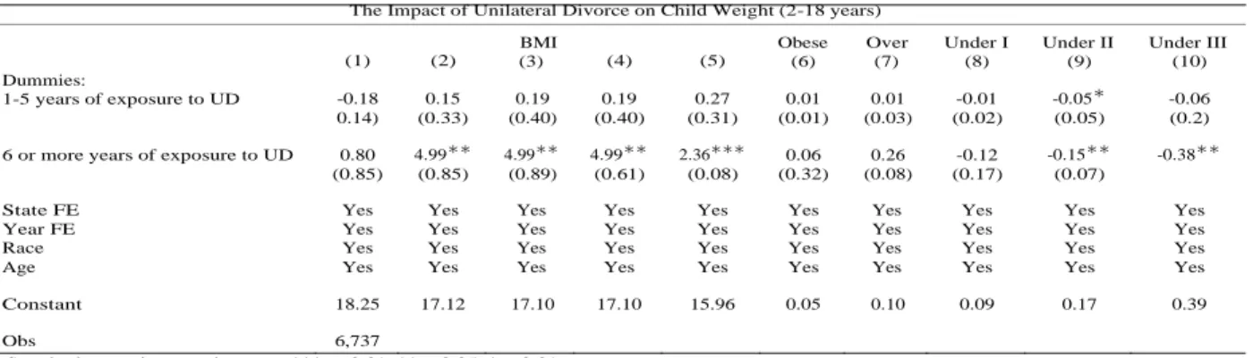
The results from Eq. (1) are presented in Table 3. Column (1) reports the result for a simple OLS regression for child BMI. Column (2) includes state fixed effects and Column (3) includes year fixed effects. Column (4) includes a set of race dummies and Column (5), which is my preferred specification, also includes a set of age dummies. The results show that children exposed to UD for 6 or more years have a higher BMI of 2.36 units, which is 14.8% of baseline. BMI is not affected by exposure to UD between 1 and 5 years.
Table 3: The Impact of Unilateral Divorce on Child Weight (2-18 years)
The Impact of Unilateral Divorce on Child Weight (2-18 years)
(1) (2) BMI (3) (4) (5) Obese (6) Over (7) Under I (8) Under II (9) Under III (10) Dummies: 1-5 years of exposure to UD -0.18 0.15 0.19 0.19 0.27 0.01 0.01 -0.01 -0.05∗ -0.06 0.14) (0.33) (0.40) (0.40) (0.31) (0.01) (0.03) (0.02) (0.05) (0.2) 6 or more years of exposure to UD 0.80 4.99∗∗ 4.99∗∗ 4.99∗∗ 2.36∗∗∗ 0.06 0.26 -0.12 -0.15∗∗ -0.38∗∗
(0.85) (0.85) (0.89) (0.61) (0.08) (0.32) (0.08) (0.17) (0.07)
State FE Yes Yes Yes Yes Yes Yes Yes Yes Yes Yes Year FE Yes Yes Yes Yes Yes Yes Yes Yes Yes Yes Race Yes Yes Yes Yes Yes Yes Yes Yes Yes Yes Age Yes Yes Yes Yes Yes Yes Yes Yes Yes Yes Constant 18.25 17.12 17.10 17.10 15.96 0.05 0.10 0.09 0.17 0.39
Obs 6,737
Standard errors in parentheses — *** p<0.01, **p<0.05, *p<0.01
The results from Column (5) indicate an increase of the child’s BMI due to the intro- duction of the divorce regime. It is important to highlight the fact that, higher BMI not necessarily indicates an unhealthy outcome. According to the CDC, a BMI is considered normal if it is between 5th and 85th percentile for their age and sex group. Therefore, a child can increase his BMI and still be under normal weight.
In order to evaluate if the impact of UD is actually making children worse, i.e, unhealthy, I run Eq. (1) with five types of dummy dependent variables: being obese, overweight and underweight types I, II and III. Column (6) and (7) present the results for the probability of being obese and overweight. Neither weight indicator is significantly affected by the intro- duction of the UD regime. Column (8) show that the the probability of being underweight type I is not affected by UD. Column (9) shows that the probability of being underweight type II decreases by 0.06 p.p. when exposed between 1 and 5 years and decreases by 0.15 p.p. when exposed to 6 or more years. Column (10) shows that the probability of being underweight type III decreases by 0.38 p.p. when exposed to 6 or more years.
The central interpretive issue with these results is the mechanisms through which UD regulation leads to outcomes. There are four possibilities, non mutually exclusive. The first candidate is parental divorce per se. The easing of divorce laws made it easier for people to leave bad marriages. A child that is exposed to their parents fight could improve, in terms of well-being,
5For more information see Binder (1983). On the variances of asymptotically normal estimators from
98 EALR, V.11, nº 1, p.88-112, Jan-Abr, 2020 when they divorce. Alternatively, having divorced parents maybe worse in terms of welfare for the child because of coordination, for example. Divorce per se, therefore, can either have a positive nor negative impact on a child’s life.
Second, UD may change the selection into marriage, which could be either positive or negative. Selection into marriage may lead to a negative selection into marriage. That is, couples of relatively low match quality are now willing to marry, reducing the average match quality of married couples and therefore increasing their marriage and divorce propensity (Alesina & Giuliano, 2007). Alternatively, since UD undermines the role of marriage as a commitment device, couples with relatively low match quality no longer marry, which increases the average quality of married couples and, therefore, decreases the marriage and the divorce propensity (Matouschek & Rasul, 2006).
Another possible channel is through changes in incentives for relationship-specific invest- ments. Marriage can be thought of as a commitment device that cultivate cooperation and induces partners to make relationship-specific investments (Matouschek and Rasul, 2006). Children (quantity) and child investment (quality) can be considered marriage-specific as- sets. The UD could reduce the incentive to allocate resources to children if couples’ incentives to make investments in relationship-specific becomes smaller.
Finally, making divorce easier can change the nature of the bargaining relationships between husband and wife. There is a large literature on development that has documented that the amount of resources allocated to children depends on the relative bargaining position between husband and wife (Strauss & Thomas, 1995; Frankenberg & Thomas, 2000). If UD weakens the bargaining position of women within marriage, children may have been negatively affected, independently of the occurrence of a divorce. If the opposite occurs, i.e, the UD weakens the bargaining position of man within marriage, then children may have been positively affected.
Now, I address the following question: does the possibility of UD affects divorce decisions? I examine both the impact on the likelihood that adults in childbearing age (25 to 45 years old) are divorced and the impact on other marital status that may be affected by this shift in legal regimes. This exercise allows me to untangle two transmission mechanisms: divorce per se and marriage. To assess the impact of UD regulations on marital status, I run regressions of the form:
where in addition to the other indexes Divorcei,j,t is a variable equals to 1 when the person i in state j
and time t is divorced (or some other marital status indicator) and equals to 0 otherwise.
The results are presented in Table 4 from Eq.(2). Column (1) reports the result for the impact of UD on the probability of being divorced including a set of individual’s age and race dummies, state fixed effects and year fixed effects. When exposed to 6 or more years to UD the probability of being divorced increases 0.10 p.p.. There is evidence, therefore, that making divorce easier increases the chance that children are more likely to be living in nontraditional families. Exposure between 1 and 5 years to UD is not significant. Column(2) and (3) report the results for the probability of being married and separated. Neither probability seems to be significantly affected by the introduction of UD.
EALR, V.11, nº 1, p.80-87, Jan-Abr, 2020 99 Table 4: The Impact of Unilateral Divorce on Marital Status (25-45 years)
The Impact of Unilateral Divorce on Marital Status (25-45 years)
(1) (2) (3)
Divorced Married Separated Dummies:
1-5 years exposure to UD 0.02 -0.00 -0.00
(0.04) (0.05) (0.01) 6 or more years of exposure to UD 0.10∗ -0.08 0.09
(0.05) (0.06) (0.07)
State FE Yes Yes Yes
Year FE Yes Yes Yes
Race Yes Yes Yes
Age Yes Yes Yes
Constant -0.00 0.78 -0.00
Obs 5,279
Standard errors in parentheses — *** p<0.01, **p<0.05, *p<0.01
The results from Eq.(2) indicate that the divorce per is acting as a transmission mech- anism from UD to child BMI. Even though the probability of being married is not affected by the UD, it is important to note that, Eq.(2) is capturing the contemporaneous effect of UD. Therefore, I cannot rule out the role of marriage as a transmission mechanism in the long term.
As mentioned before, the present work investigates the impact of an easier divorce process on several marital status indicators. It is important to highlight that NHANES I is a sample whose goal is to understand the health status of the US, therefore, it is not ideal for this exercise. Additionally, I believe the previous work have better data and have done a fine job uncovering the impact of UD on marital status indicators, which is postive and in line with Gruber (2004) and Wolfers (2006).
5.1.2. Children between 7 and 18 years
One concern with the approach described in Section 5.1.1 is that there are several transmis- sion mechanisms from UD to child outcome. As said before, a child can be affected by several channels. In order to minimize the effect of some of those mechanisms, I estimate Eq.(1) for children between 7 to 18 years old. But, it is important to note that it is not appropriate to extrapolate the results for children in general, once this approach also introduces age specific effects problem. It could be the case that the impact of UD is not homogeneous across ages.
In this specific age group 99% of than where born before the UD regime. Therefore, I can rule out (or at least decrease at its maximum) the effect of selection bias into marriage, once the parents got married before the UD. It is also possible to rule out changes in the relationship specific-investments, since those choices were already made before the child’s birth. The remaining mechanisms are divorce per se and changes in the bargaining position.
100 EALR, V.11, nº 1, p.88-112, Jan-Abr, 2020 The results are presented in Table 5. Column (1) reports the result for children BMI for an OLS regression including a set of individual’s age and race dummies, state fixed effects and year fixed effects. Children exposed to UD for 6 or more years have higher BMI by 3.77 units, which is 25.8% of baseline. BMI is not affected by exposure to UD between 1 and 5 years.
Table 5: The Impact of Unilateral Divorce on Child Weight (7-18 years) The Impact of Unilateral Divorce on Child Weight (7-18 years)
(1) (2) (3
) (4) (5) (6)
BMI Obese Over Under I Under II Under III Dummies:
1-5 years of exposure to UD 0.40 0.02 0.02 -0.01 -0.08∗∗ -0.02
(0.39) (0.02) (0.03) (0.03) (0.03) (0.06) 6 or more years of exposure to UD 3.77∗∗∗ -0.03 0.87∗∗∗ -0.03 -0.08∗∗ -0.15∗∗
(0.45) (0.02) (0.07) (0.04) (0.04) (0.07)
State FE Yes Yes Yes Yes Yes Yes
Year FE Yes Yes Yes Yes Yes Yes
Race Yes Yes Yes Yes Yes Yes
Age Yes Yes Yes Yes Yes Yes
Constant 14.62 -0.01 0.03 0.16 0.15 0.35
Obs 3,977
Standard errors in parentheses — *** p<0.01, **p<0.05, *p<0.01
I then consider 5 other weight indicators: being obese, overweight and underweight types I, II and II. Column (2) present the result for the probability of being obese, which is not significant. Column (3) presents the results for the probability of being overweight, which increases by 0.87 p.p. when the child is exposed to 6 or more years to UD. Column (4) shows that the probability of being underweight type I is not affected by the UD. Column
(5) shows that the probability of being underweight type II is lower by 0.08 p.p. when the child is exposed between 1 and 5 years to UD and lowers 0.08 p.p. when exposed for at least 6 years. Column (6) reports the result for the probability of being underweight type III. Children exposed to 6 or more years to UD have 0.15 p.p. lesser chance to be underweight type III.
The results found in this Section suggest that the effects of the remaining mechanisms for this age group, divorce per se and changes in the bargaining, are negative if I compare with the results found in Section 5.1.1. In Section 5.1.1 the results indicate an increase in the BMI and lower probability to be underweight. In this Section the results also show an increase in the BMI and lower probability to be underweight, but now there is also the increase in the probability to be overweight. The conclusion from these results is that the mechanisms divorce per se and changes in the bargaining have a negative effect on child health.
5.1.3. Children between 2 and 6 years
The introduction of UD can affect a child’s health through several transmission mechanisms. It is important to note, however, that depending on the child’s age, the channels of trans- mission from UD to child weight should differ.
EALR, V.11, nº 1, p.80-87, Jan-Abr, 2020 101
i,j,t
In Section 5.1.1, the results showed that children between 2 and 18 years old are increasing their BMI and being less likely to be underweight types II and III. However, children between 2 years and 18 years are different. Younger children are less independent when compared to older kids. It is reasonable to believe that older kids have more “food independence”, meaning that they can choose more freely the type and amount of food they want to eat. The opposite should occur to younger children, since they do not have food independence when compared to older children. Therefore, the changes on the weight of younger children can be attributed mostly to parents influence. If a three year old child is putting on unhealthy weight, for example, it is plausible to assume that what is causing this change is parental influence, in its majority, not because this child decided to eat more or with less quality. On the other side, if a younger child is getting into better shape, it is probably because the parents are paying more attention to it.
In order to analyze the different channels I also run another specification for three age groups of younger children (2 to 4, 2 to 5; 2 to 6):
WMi,j,t = α0 + α1DExpi,j,t + X α2 + δt + λj + εi,j,t (3)
where, in addition to the other indexes, DExpi,j,t is a dummy for the presence of a unilateral reform
law in the year the NHANES interview or in the previous years. Once the child’s age ranges from 2 to 6 years old, it does not make sense to use a dummy variable that indicates the presence of at least 6 years of exposure to UD. Therefore, this specification is slightly different from the one in Eq.(1).
The results are presented in Table 6. Columns (1)-(6) report the result for children between 2 and 4. Columns (7)-(12) show the result for children between 2 and 5. And Columns (13)-(18) report the result for children between 2 and 6. All of the regressions include a set of individual’s age and race dummies, state fixed effects and year fixed effects.
The age group composed of 2 and 4 years old, is the less independent, and the impact of an easier divorce process is not significant. When I add 5 year old children, the results remains the same. This last group, of 2 to 5 years olds, is comprise with more independent children. However, still plausible to believe that 2 and 5 year olds are very influenced by parents decisions. Finally, the UD reduces the probability of being underweight type III by 0.13 p.p., for the group of 2 and 6 years, therefore, increasing the child’s health. The group composed of 2 and 6 years old children is composed with even more independent children. Its plausible to assume that 2 and 6 year olds are massively influenced by their parents decisions. Only for the group of 2 and 6 years I find that the UD increases health, however the results are very sensitive to age group.
In Section 5.1.2 I estimate Eq.(2) with children between 7 and 18 years old to shut down two possible transmission mechanisms: selection into marriage and marriage-specific investment. Therefore, is straightforward that when I estimate Eq.(3) with children between 2 and 6 years old there is the presence of the four transmission mechanisms. The results of this Section should be read with careful once there are too many forces acting here: the presence of the age specific effects and two additional transmission mechanism (selection into marriage and marriage-specific investment).
102 EALR, V.11, nº 1, p.88-112, Jan-Abr, 2020
Table 6: The Impact of Unilateral Divorce on Child Weight
The Impact of Unilateral Divorce on Child Weight
2 and 4 year 2 and 5 year 2 and 6 year
(1) (2) (3) (4) (5) (6) (7) (8) (9) (10) (11) (12) (13) (14) (15) (16) (17) (18) BMI Obese Over Under I Under II Under III BMI Obese Over Under I Under II Under III BMI Obese Over Under I Under II Under III Exposed 0.06 (0.23) 0.01 (0.02) -0.0 (0.05) -0.02 (0.02) -0.03 (0.06) -0.11 (0.08) -0.03 (0.20) 0.01 (0.03) -0.01 (0.04) 0.01 (0.02) 0.03 (0.05) -0.10 (0.07) -.-1 (0.19) -0.01 (0.02) -0.02 -0.00 (0.04) (0.03) -0.00 (0.01) -0.13∗∗ (0.06) State FE Yes Yes Yes Yes Yes Yes Yes Yes Yes Yes Yes Yes Yes Yes Yes Yes Yes Yes Year FE Yes Yes Yes Yes Yes Yes Yes Yes Yes Yes Yes Yes Yes Yes Yes Yes Yes Yes Race Yes Yes Yes Yes Yes Yes Yes Yes Yes Yes Yes Yes Yes Yes Yes Yes Yes Yes Age Yes Yes Yes Yes Yes Yes Yes Yes Yes Yes Yes Yes Yes Yes Yes Yes Yes Yes Constant 16.93 0.13 0.21 0.09 0.15 0.27 17.15 0.10 0.23 0.02 0.05 0.22 17.10 0.12 0.23 0.06 0.06 0.29
Obs 1,696 2,280 2,760
Standard errors in parentheses — *** p<0.01, **p<0.05, *p<0.01
i,j,t i,j,t i,j,t i,j,t i,j,t i,j,t 5.2 Robustness Checks
In this section, I undertake several robustness checks. The first potential threat to the results arises from the possibility that estimated effects may reflect a specification bias. I run several specifications to analyze if and how the results change.
First, Table 7 presents the results for Eq.(1) using the whole sample of children, 2 to 18 years, instead of only 2 and 6 years. Column (1) reports the results for child BMI, Column (2) for probability of being obese, Column (3) for probability of being overweight, Column (4) for probability of being underweight type I, Column (5) for probability of being underweight type II and Column (6) for the probability of being underweight type III. Independently of the weight measure, the variable DExpi,j,t is not significant. The only exception is the probability of being
underweight type II. Children expose to UD have lower 0.05 p.p. chance to be underweight type II.
Table 7: The Impact of Unilateral Divorce on Child Weight (2-18 years) The Impact of Unilateral Divorce on Child Weight (2-18 years)
(1) (2) (3) (4) (5) (6)
BMI Obese Over Under I Under II Under III
Exposed 0.28 0.01 0.01 -0.01 -0.05∗∗ -0.06
(0.31) (0.01) (0.03) (0.01) (0.02) (0.05)
State FE Yes Yes Yes Yes Yes Yes
Year FE Yes Yes Yes Yes Yes Yes
Race Yes Yes Yes Yes Yes Yes
Age Yes Yes Yes Yes Yes Yes
Constant 15.97 0.05 0.10 0.08 0.15 0.36
Obs 6,737
Standard errors in parentheses — *** p<0.01, **p<0.05, *p<0.01 I also test a new equation which is similar to Eq. (1) with a simple difference:
WMi,j,t = α0 + α1Exp1 to x + α2Expx+1 or more + X α3 + δt + λj + εi,j,t (4)
i,j,t i,j,t i,j,t
where, in addition to the other indexes, Exp1tox equals to 1 if the person i in state j and time t
was exposed to UD from 1 to x years; and equals to 0 otherwise. The variable Expx+1ormore
equals to 1 if the person had equal or more then (x + 1) years of exposure to UD; and equals to 0 otherwise. The variable x ranges from 2 to 4.
Table 8 presents the results from Eq. (4). Column (1) report the results using two dummies, exposure to UD between 1 and 2 years (Exp1to 2) and exposure for 3 years or more (Exp3ormore).
Column (2) show the results using exposure to UD between 1 and 3 years (Exp1 to 3) and
exposure for 4 years or more (Exp4ormore). Finally, Column (3) show the results using exposure to
104 EALR, V.11, nº 1, p.88-112, Jan-Abr, 2020
Table 8: The Impact of Unilateral Divorce on Child BMI (2-18 years)
The Impact of Unilateral Divorce on Child BMI (2-18 years)
(1)
(2)
(3)
Dummies:
1-2 years exposure to UD
0.30
(0.31)
3 or more years of exposure to
UD
0.45
(0.40)
1-3 years exposure to UD
0.28
(0.31)
4 or more years of exposure to
UD
0.48
(0.36)
1-4 years exposure to UD
0.28
(0.31)
5 or more years of exposure to
UD
2.06
∗∗∗(0.69)
State FE
Yes
Yes
Yes
Year FE
Yes
Yes
Yes
Race
Yes
Yes
Yes
Age
Yes
Yes
Yes
Obs
6,135
The constant variable is 15.96 for all
specifications Standard errors in
parentheses
*** p<0.01, **p<0.05, *p<0.01
The results from Columns (1)-(2) show no impact of UD on child BMI. Column (3), however, shows a similar result to the ones found in section 5.1.1. When exposed for at least 5 years to UD the child BMI increases by 2.06 units.
Finally, there is a concern that the results are driven by outlier states. The obvious candidate is California, once its a large state and was one of the firsts to allow the UD. The basic pattern of results, however, remains the same, as can be seen in Table 9.
j
j
Table 9: The Impact of Unilateral Divorce on Child Weight (without California) (2-18 years) The Impact of Unilateral Divorce on Child Weight (without California) (2-18 years)
Dummies: BMI Obes e Over Under I Under II Under III 1-5 years exposure to UD 0.32 0.01 0.01 -0.02 -0.06∗∗ -0.06 (0.32) (0.01) (0.03) (0.01) (0.02) (0.05) 6 or more years of exposure to
UD
2.31∗∗∗ 0.06 0.25 -0.12 -0.15∗∗ -0.37∗∗ (0.64) (0.08) (0.32) (0.08) (0.07) (0.17)
State FE Yes Yes Yes Yes Yes Yes
Year FE Yes Yes Yes Yes Yes Yes
Race Yes Yes Yes Yes Yes Yes
Age Yes Yes Yes Yes Yes Yes
Constant 15.91 0.05 0.09 0.09 0.17 0.40
Obs 6,135
Standard errors in parentheses — *** p<0.01, **p<0.05, *p<0.01
5.3 Validating the Empirical Strategy
The empirical strategy employed in this paper exploits time and state variation in the adop- tion of the UD. The underlying assumption is that the timing of introduction of UD is not correlated with child health, meaning weigh. To test whether this hypothesis is valid I have also pursued a series of specification checks to assess whether I am truly uncovering a causal impact of UD regulations.
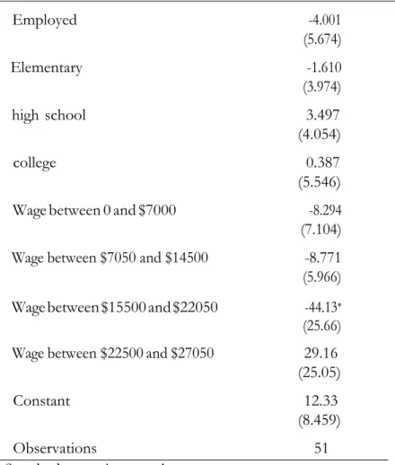
One concern is that there are somehow other omitted state variables that are correlated with the passage of UD regulations. I have gathered data from the The Integrated Public Use Microdata Series (IPUMS-USA). The IPUMS consists of over sixty high-precision samples of the American population drawn from sixteen federal censuses, from the American Com- munity Surveys of 2000-present. To test the hypothesis that the timing of introduction of the UD is not correlated with state characteristics is valid, I collect a few socio demographic characteristics of the state’s population from 1960. I examine whether characteristics be- tween treated and non-treated states are different before the establishment of the UD. The econometric model is:
Y 1960 = α + βDExpj + εj (5)
where in addition to the other indexes Y 1960 represents a set of socio demographic character-
106 EALR, V.11, nº 1, p.88-112, Jan-Abr, 2020 One obvious candidate of omitted variable is education. It is possible that UD were being passed in states where there was less educational levels, once again leading to more adverse child health outcomes. The results in Table 10 show no significant correlation with the pres- ence of UD in the 70’s. Another candidate is income. Using the same strategy, as mentioned before, I once again find no significant correlation with the presence of UDs.
Table 10: Test of Difference in Means (Treatted vs. Non Treated) Test of Difference in Means (Treatted vs. Non Treated)
Employed -4.001 (5.674) Elementary -1.610 (3.974) high school 3.497 (4.054) college 0.387 (5.546)
Wage between 0 and $7000 -8.294
(7.104) Wage between $7050 and $14500 -8.771 (5.966) Wage between $15500 and $22050 -44.13∗
(25.66)
Wage between $22500 and $27050 29.16
(25.05)
Constant 12.33
(8.459)
Observations 51
Standard errors in parentheses *** p<0.01, **p<0.05, *p<0.01
Another way to check whether my empirical strategy is valid is to add income and education as control variables in the equations. The results do not alter, corroborating that the timing of introduction of UD is not correlated with the omitted variables mentioned before.
6. Discussion
The first American state to allow the UD was New Mexico in 1933, and in the sequence, Alaska in 1935. The majority of states, however, changed their regulation in the 70’s. In the variation between 1971 and 1974, which is the period studied in this paper, 19 states changed their regulations to UD, totaling 28 states. Since mid-1970s most states in the USA allowed for UD, which allowed divorce with the consent of just one rather then both spouses.
In order to assess the impact of the UD on child weight gain, I analyze a comprehensive nationwide health and nutrition examination survey during 1971–1974. I use difference-in- differences approach using the variation resulting from the differences in the timing of the adoption of UDs across the adopting states. The results indicate that after the introduction of the UD, children between 2 and 18 years old have bigger BMI and lower probability of being underweight types II and III. According to CDC, a BMI is considered normal if it is between 5th and 85th percentile for their age and sex group. Therefore, according to the CDC, the results indicate that children affected by the UD still under normal weight. However, having lower probability of being underweight type II means to have a lower probability of having a BMI below the 10th percentile, which could also be an indicator of getting healthier.
The results paint an interesting picture of the exposed children. The previous literature (Yannakoulia, et al., 2008; Kimbro, 2013; Biehl et al., 2014) showed evidence that children are at greater risk of being obese because they are living outside of an intact family. My results, however, do not go in the same direction. Exposure to UD do not leads to weight gain, in a conservative analysis. But in a more detailed analysis, exposure to UD leads to better health for children between 2 and 18 years old. The central interpretive issue with these results is the mechanisms through which UD regulation leads to the outcomes.
It is worth noting that the UD affects BMI through several channels. Therefore, when all the mechanisms are present, the final effect of making divorce easier is positive for the child. Children’s well-being can be affected through different channels. The most common candidate is parental divorce per se.The UD made it easier for people to leave unsuccessful marriages. A child that is exposed to their parents fight could improve in terms of well-being, when they get a divorce. Alternatively, having divorced parents maybe worse in terms of welfare for the child because of coordination, for example. A higher incidence of divorce could imply that a higher proportion of children have faced this event and are therefore forced to live under nontraditional family structure. Divorce per se, therefore, can either have a positive nor negative impact on a child’s life.
Moreover, UD may change the selection into marriage. On the one hand, it may lead to a negative selection into marriage. Couples of relatively low match quality are now willing to marry, which reduces the average match quality of married couples and increases their marriage and divorce propensity (Alesina & Giuliano, 2007). On the other hand, couples with relatively low match quality no longer marry, once UD undermines the role of marriage as a commitment device, which increases the average quality of married couples and, therefore, decreases the marriage and the divorce propensity (Matouschek & Rasul, 2006).
Another possible channel is through changes in incentives for relationship-specific invest- ments. Marriage can be thought of as a commitment device that cultivate cooperation and induces partners to make relationship-specific investments (Matouschek & Rasul, 2006). The amount of children and their ”quality” can be considered marriage-specific assets. The UD could reduce the incentive to allocate resources to children if couples’ incentives to make investments in relationship-specific becomes smaller. However, a higher incentive to make market-specific investments such as labor employment (Stevenson, 2007), may increase the amount of resources available for children.
Finally, making divorce easier can change the nature of the bargaining relationships be- tween husband and wife. There is vast literature on development that has documented that the amount of resources allocated to children depends on the relative bargaining position between husband and wife (Strauss & Thomas, 1995; Frankenberg & Thomas, 2000). There- fore, if UD weakens the bargaining position of women within marriage, children may have been negatively
108 EALR, V.11, nº 1, p.88-112, Jan-Abr, 2020 affected, independently of the occurrence of a divorce.
In order to try to understand the transmission mechanisms, I study children between 7 to 18 years old. In this specific age group. the majority where born before UD implementation. The idea is to rule out selection bias into marriage, once the parents got married before the UD law. It is also possible to rule out changes in the relationship specific-investments, since those choices regarding the relationship investments were already made before the child’s birth. But, it is important to keep in mid that I also introduce age specific effects problem. The remaining mechanisms, therefore, were divorce per se and changes in the bargaining position.
The results indicate that exposure to UD no longer leads to better health for children between 7 and 18 years. Exposed children had higher BMI, bigger probability to be over- weight and lower probability to be underweight type II. Following the definitions of healthy weight from the CDC, the introduction of UD had an overall negative impact on child health, once underweight type II still is consider normal weigh. It is important to remember that, the result for older children can not be generalized, once the majority were born under the no-fault divorce law. The next generation will be born under the UD. The extrapolation exercise should not be done. However, using my indicator of underweight, the results can be considered mixed. On the one hand, there is a lower probability to be underweight type II. On the another hand, there is a bigger probability to be overweight.
When I compare the results for children between 7 and 18 years and children between 2 and 18 years the results suggest that the effects of the remaining mechanisms for the first age group, divorce per se and changes in the bargaining, are negative. The results for children between 2 and 18 years indicate an increase in the BMI and lower probability to be underweight. However, the results for children between 7 and 18 years also show an increase in the BMI and lower probability to be underweight, but now there is also the increase in the probability to be overweight. The conclusion from these results is that the mechanisms divorce per se and changes in the bargaining have a negative effect on child health.
Another concern is that, depending on the child’s age, the channels of transmission from UD to child weight should also differ. On the one hand, there is the direct parental influence: parents can influence their children through several ways (Benton, 2004). First, there is the food as reward. Parents can offer of one food (dessert) as a reward for the eating of another (vegetables). Second, there is the limit access to food, where the child is simply not allowed to eat a certain type of food (candies, chocolate, etc). And finally, there is the parental example, i.e, parents eating healthy food in front of the children. Snoek, Sessink & Engels (2010) indicates that family food patterns might have great impact already at young ages.
Moreover, there is the child own will as a mechanism. It is plausible to assume that as the child becomes older, he/she also becomes more independent, in terms of feeding. It is straightforward to infer that, external events can play a crucial role determining the type and amount of food the child is eating. Exposure to traumatic events during childhood is associated with an elevated risk of adult obesity (Gunstad, Paul, Spitznagel, Cohen, Williams, Kohn & Gordon, 2006; Felitti, Anda, Nordenberg, Williamson, Spitz, Edwards, Koss & Marks, 1998).
Since I cannot separate these two channels, parental influence vs. child own will, I analyze three group of young children (2 to 4; 2 to 5 and 2 to 6). The groups are made so the first group is comprised of more dependent children than the second group, and second group is comprised of more dependent children than the third group. It is reasonable to assume that, the younger the child, the strongest the parental influence. Therefore, the results from this exercise can be interpreted as ”cleaned” from child own will effects. Once again, according to CDC there is no
evidence that younger kids are changing their weight. However, following my definition of underweight, there is a weak evidence that younger kids are getting healthier, meaning smaller probability to be underweight type III. It is important to note that, when I estimate with children between 2 and 6 years old there is the presence of the four mechanisms. The results for this age group should be read with careful once there are too many forces acting here: the presence of the age specific effects and two more transmission mechanisms (selection into marriage and marriage-specific investment) when compared to children between 7 and 18 years.
I undertake several robustness checks. The first potential threat to the results arises from the possibility that estimated effects may reflect a specification bias. I first tried to capture the impact of the UD through a unique dummy variable (any exposure to UD). The results showed that independently of the weight measure the impact of UD was not significant. This result is not surprising since an unique dummy variable assumes that the impact of UD is the same for all the affected sample. The specification that uses only one dummy variable probably do not represents what actually happens, once one would expect that different lengths of exposure should have different impacts on child health. Its reasonable to assume that one year of exposure to UD should have a different impact of 10 years of exposure. Moreover, California is a obvious to be an outlier state. Once its a large state and was one of the firsts states to allow the UD. The basic pattern of results, however, remains the same.
7. Conclusion
In this paper, I investigate whether the UD affects child health through weight gain. I use difference-in-differences approach using the variation resulting from the differences in the timing of the adoption of UD across the adopting states. To assess the impact of UD on child health, I analyze the NHANES I during 1971–1974. My results do not show that the introduction of UD leads to unhealthy weight gain. Children are putting on more weight, however they still under the normality patterns established by the CDC. I also verify if the UD affects the marital status. The impact of UD is positive on the probability of being divorced when the person is in childbearing age. The probability of being married and separated is not affected.
The UD can dissolve the marriage contract and, therefore, the unilateral reform can be seen as a change in those marriage contracts already in place at the time of the reform. Therefore, the change in legislation should produce different effects over those individuals who had taken marriage or investment decisions based on mutual consent divorce rules. Even though those effects are transitional overall, they may become permanent for children of those families caught in the transition. In order to analyze the behavior of couples who had taken marriage or investment decisions based on mutual consent divorce rules, I consider children between 7 and 18 years. This age group is mostly composed of children born before the introduction of the UD. The results, following the definition of BMI established by the CDC, indicate that children that were born before the introduction of the UD are becoming less healthier.
Moreover, it is important to note that, depending of the child’s age, the channels of transmission from UD to child weight should differ. Older children may have more food independence, meaning that they can choose more freely the type and amount of food they want to eat. The opposite should occur to younger children, once they are not completely independent. Younger children should be largely influenced by their parents choices. There- fore, changes in the weight of younger children can be attributed mostly to parents influence. The results, also following the CDC definitions, indicate that younger children are not chang- ing their weight after the UD.
110 EALR, V.11, nº 1, p.88-112, Jan-Abr, 2020 This is the first paper in the literature, to the best of my knowledge, to examine the impact of UD on child health, meaning child weight. Further research is necessary to un- derstand and perhaps estimate the transmission mechanism from divorce laws through child outcome.
8. References
Adda, J., & Cornaglia, F. (2010). The effect of bans and taxes on passive smoking. American Economic Journal : Applied Economics, 2(1), 1-32.
Allen, D. W. (1992). Marriage and divorce: Comment. The American Economic Review, 82(3), 679-685.
Almond, D., Hoynes, H. W., & Schanzenbach, D. W. (2011). Inside the war on poverty: The impact of food stamps on birth outcomes. The Review of Economics and Statistics, 93(2), 387-403.
Anger, S., Kvasnicka, M., & Siedler, T. (2011). One last puff? Public smoking bans and smoking behavior. Journal of Health Economics, 30(3), 591-601.
Benton, D. (2004). Role of parents in the determination of the food preferences of children and the development of obesity. International journal of obesity, 28(7), 858- 869.
Bharadwaj, P., Johnsen, J. V., & Løken, K. V. (2014). Smoking bans, maternal smoking and birth outcomes. Journal of Public Economics, 115, 72-93.
Biehl, A., Hovengen, R., Grøholt, E. K., Hjelmesæth, J., Strand, B. H. & Meyer, H. (2014). Parental marital status and childhood overweight and obesity in Norway: a nationally representative cross-sectional study. BMJ open, 4(6).
Binder, D. A. (1983). On the variances of asymptotically normal estimators from complex surveys. International Statistical Review/Revue Internationale de Statistique, 51(3), 279-292.
Briggs, R. J. (2009). The Impact of Smoking Bans on Birth Weight: Is Less More?Working paper. Bjorklund, A., & Sundstr¨om, M. (2006). Parental separation and children’s educational attainment: A
siblings analysis on Swedish register data. Economica, 73(292), 605-624.
Colman, G., Grossman, M., & Joyce, T. (2003). The effect of cigarette excise taxes on smoking before, during and after pregnancy. Journal of Health Economics, 22(6), 1053-1072.
Dietz, P. M., Homa, D., England, L. J., Burley, K., Tong, V. T., Dube, S.R. & Bernert, J. T. (2011) Estimates of Nondisclosure of Cigarette Smoking Among Pregnant and Non-pregnant Women of Reproductive Age in the United States. American Journal of Epidemiology, 173(3), 355-359.
Dolan-Mullen, P., Ramirez, G., & Groff, J. Y. (1994). A meta-analysis of randomized trials of prenatal smoking cessation interventions. American Journal of Obstetrics and Gynecology, 171(5), 1328-1334.
Felitti, V. J., Anda, R. F., Nordenberg, D., Williamson, D. F., Spitz, A. M., Edwards, V., & Marks, J. S. (1998). Relationship of childhood abuse and household dysfunction to many of the leading causes of death in adults: The Adverse Childhood Experiences (ACE) Study. American Journal of Preventive Medicine, 14(4), 245-258.