FINAL dissertation
Risk neutral and real world densities for
the S&P 500 index during the crisis
period from 2008 to 2009
IMScBA (Corporate Finance and Control)
Name: Ping Sun
Student No. 152110152
Words count: 10,482
Risk neutral and real world densities for
the S&P 500 index during the crisis
period from 2008 to 2009
Abstract
Risk neutral and real world densities derived from option prices provide rich source of information for future asset price forecast. Three approaches (mixtures of two lognormals, jump diffusion models and implied volatility function models) are used to estimate risk neutral densities. Both power utility function and beta function are used to transform mixtures of two lognormal risk neutral densities into real world densities. Transformations are estimated by maximizing the likelihood of observed index levels. Results for the S&P 500 index indicate that two parametric methods, especially the jump diffusion models are preferable than implied volatility function methods. The log-likelihood tests cannot reject the hypothesis that there is no risk premium for both year 2008 and year 2009.
Table of Content
Section I Introduction ... 1
Section II Literature Review ... 3
2.1 Implied Volatility ... 3
2.2 Risk-neutral Density ... 4
2.2.1 Methods to obtain RND ... 5
Parametric methods ... 5
Non-parametric methods ... 8
Comparison of different methods ... 10
2.2.2 Applications of RND ... 11
2.3 Real World Density ... 12
Section III Methodology ... 14
3.1 RND estimation methods ... 14
Mixtures of lognormal method ... 14
Jump-diffusion model... 15
Implied Volatility Function method ... 16
3.2 Risk transformation methods ... 17
Transformation from utility function ... 18
Transformation from calibration function ... 18
Mixtures of lognormal densities transformation ... 19
3.3 Estimation of the RND and the transformation parameters ... 21
Section IV Data Description ... 22
Section V Empirical Results of RND ... 24
5.1 Average pricing errors of various methods... 24
5.2 Moments of RNDs for various methods ... 25
5.3 Moments of RNDs during different periods... 27
5.3.1 RND on April 19, 2008 ... 27
5.3.2 RND on September 20, 2008 ... 29
5.3.3 RND on April 18, 2008 ... 31
5.4 Parameter estimates of the Jump Diffusion model ... 33
Section VI Empirical results of Real World Density ... 35
6.1 Parameter estimation of power utility function transformation ... 35
6.2 Parameter estimation of beta function transformation ... 37
6.3 The likelihood-ratio test ... 38
6.4 Comparison of RNDs and Real World Densities ... 39
6.5 Comparison of the moments for RNDs and Real World Densities ... 41
Section VII Conclusion ... 44
Appendix ... i
Section I Introduction
In the fall of 2008, the bankruptcy of large independent investment banks such as Lehman Brothers caused a global wave of panic selling, and this quickly turned into a wide spread global financial crisis. This worldwide financial crisis began in the summer of 2007 in the U.S. credit market, and particularly the market for the mortgage-backed collateralized debt obligations (Birru & Figlewski, 2010). However, the stock market reflected the crisis neither properly nor immediately. The economy has been widely considered to enter a recession since December of 2007, while the S&P 500 index level was still around 1300 at the end of August of 2008 (Birru & Figlewski, ibid). Since September of 2008, the U.S stock markets, including S&P 500 index has experienced sharp declines. The markets were highly uncertain and highly volatile during that period. As a result, investors lowered both their expectations and their willingness to bear risk.
Compared with time series of asset prices, option prices are regarded to be more informative and are able to better gauge the market sentiment. Therefore, the risk-neutral density obtained from sets of option prices is able to reflect better both the investors‘ feelings about future evolutions of the underlying assets, and also their objective estimations of the underlying assets‘ probability distribution on the options expiration date. Furthermore, the real world density transformed from the risk-neutral density provides deep insight into investors‘ attitudes towards risk. This paper tends to explore how the investors‘ expectations are reflected in the behavior of the risk-neutral densities during this extraordinary period. In addition, by transforming risk-neutral densities into real world densities, the risk preferences of investors will also be examined. The paper concerns the comparison of different methods of extracting the risk-neutral densities and the relationship between risk-neutral and real world densities.
The following Section provides a brief literature review, including studies on implied volatilities, literatures about methods of extracting risk-neutral densities and applications of the risk-neutral densities, and also the studies on obtaining the real world density and implied risk aversion. Section III describes the methodologies this paper uses to estimate both the risk-neutral densities and the risk aversion from option prices. Section IV describes the S&P 500 index option prices, risk free rates and dividend yields uses in the analysis. In Section V, the primary empirical results of risk-neutral densities are presented and interpreted, including a general comparison of different approaches to extract risk-neutral densities, time-series comparison, and estimated parameters explanation. Section VI focuses on the empirical results of real world densities and risk aversion parameters. This Section starts with the risk parameters explanation, and is followed by the likelihood ratio tests, the comparison of moments between risk-neutral densities and real world densities. Finally, Section VII provides a conclusion.
Section II Literature Review
2.1 Implied volatilityGiven their forward-looking nature and corresponding to a sufficient range of strike prices, option prices provide a rich source of information for estimating market perceptions of underlying asset prices when the options expire. Initially, investors reversed the process of obtaining prices from the Black-Scholes model to work out the implied volatilities of options (Jackwerth, 2004). The ability of implied volatility to predict the future underlying asset volatility has been extensively discussed (Anagnou et al, 2002; Pérignon & Villa, 2002). Latané & Rendleman (1976), Trippi (1977), Chiras & Manaster (1978) and Beckers (1981) examined the implied volatilities of common stock options. Later, more emphasis was placed on stock index options. Most of the studies including Day & Lewis (1988, 1990), Lamoureux & LaStrapes (1991), Harvey & Whaley (1992), Canina & Figlewski (1993), Fleming (1993), and Christensen & Prabhala (1998) observed S&P 100 stock index. Meanwhile, Park & Sears (1985) and Feinstein (1989) considered the options on S&P 500 index futures. Furthermore, some researches emphasized the options on other financial assets such as German Government Bond (Neuhasu, 1995) and currency futures (Jorion, 1995). These studies obtained contradictory results. For S&P 100 stock index market (Canina & Figlewski, ibid) and German Government Bond market (Neuhaus, ibid), the implied volatility seemed to provide little information for future realized volatility forecast. On the other hand, Christensen & Prabhala (ibid) and Jorion (ibid) concluded the substantial predictive power of implied volatility for both S&P 100 stock index and currency futures. Nonetheless, almost all studies reached a similar conclusion that the implied volatility suffered from upward bias (Anagnou et al, ibid; Jackwerth, ibid).
In addition to the upward bias, implied volatility also violates the constant variance assumption of the Black-Scholes model (Pérignon & Villa, 2002; Jackwerth, 2004). With respect to the strike prices, the market implied volatilities of options often present a skewed structure, called implied volatility smiles (Pérignon & Villa, ibid; Jackwerth, ibid). A majority of studies focusing on the stock index options supported the implied volatility smile effect, for instance in Rubinstein (1994) for the U.S. stock index, in Tompkins (2001) for the Japanese, German and British stock indexes, in Navatte & Villa (2000) for the French stock index, and in Pena et al (1999) for the Spanish stock index. Moreover, Rubinstein (1985) found slightly U-shaped volatility smiles for options on individual U.S. stocks, whereas the violations of the Black-Sholes model were mainly within the bid-ask spreads. Meanwhile, Mayhew (1995), Toft & Prucyk (1997) and Dennis & Mayhew (2002) reported the downward-sloping volatility smiles for individual stocks options, which were not as steep as in the index smiles. Other markets, such as foreign exchange options (Campa et al, 1998) and interest rate markets, exhibit U-shaped volatility smiles. Additionally, Jarrow et al (2003) found a downward-sloping volatility smile for options on the interest rate caps market. Due to the upward bias and the smile effect of implied volatility, more informative models are required by investors in order to estimate future underlying asset prices.
2.2 Risk-neutral density
In recent years, attention has shifted from obtaining implied volatility to deriving the whole distribution of the future underlying asset price. The extracted distribution is the risk-neutral probability distribution (RND) (Pérignon & Villa, 2002). According to the arbitrage pricing theory, in a risk-neutral environment, the current price of each security is equal to the present value of its expected payoffs discounted by a risk free interest rate, and hence RNDs can be extracted by using the observed option prices
(Taylor, 2005; Monteiro et al, 2008). Ross (1976) firstly provided an insight that a complete set of European option prices could be used to obtain RNDs. Later, Banz & Miller (1978) and Breeden & Litzenberger (1978) proposed that RND was equal to the second derivative of option prices with respect to strike prices. Since the payoffs of options depend on the future values of the underlying asset, the implied RND is a forward-looking forecast of the underlying asset‘s probability distribution (Monteiro et al, ibid). Studies about both the methods to extract the risk-neutral density and the applications of risk-neutral density will be summarized respectively.
2.2.1 Methods to obtain risk-neutral density
Many methods for implied risk-neutral density estimation have been developed. Generally, they can be divided into two basic categories: parametric and non-parametric methods.
Parametric methods
The parametric approaches assume that the RND belongs to a general distribution family, and then try to fit the observed option prices into this assumed distribution to identify the unknown parameters (Anagnou et al, 2002). Within these parametric methods, four sub-groups can be identified—mixture methods, expansion methods, generalized distribution methods and stochastic process methods.
1. Mixture methods
A mixture of two lognormal densities is first proposed by Ritchey (1990). The density is a weighted combination of lognormal densities. Lognormal mixtures have been widely used, for instance in Bahra (1997), Söderlind & Svensson (1997) and Coutant et al (2001) for interest rates, in Campa et al (1998), Jondeau & Rockinger (2000) for exchange rates, and in Gemmill & Saflekos (2000), Bliss & Panigirtzoglou (2002), Anagnou et al (2002) and Liu
et al (2007) for equity indexes. In addition, a mixture of three lognormals
with seven parameters is used by Melick & Thomas (1997) to estimate the prices of crude oil futures during the Gulf War. The mixture methods are fairly easy to apply and preferred by the policy-makers in quite a few industrialized nations (Anagnou et al, ibid; Taylor, 2005). Moreover, they are flexible to allow quite a wide range of shapes (Anagnou et al, ibid; Taylor,
ibid). However, the added flexibility results in quickly increasing the number
of parameters (Jackwerth, 2004).
2. Expansion methods
Expansion methods have strong theoretical foundations and are conceptually related to Taylor series expansions for simple functions (Jackwerth, 2004). The starting point of these methods is a simple probability distribution, then the correction terms are added (Jackwerth,
ibid). The Edgeworth expansion method is developed by Jarrow & Rudd
(1982). Corrado & Su (1996) described the underlying RNDs with a Gram-Charlier expansion approximation. In a similar spirit, Abadir & Rockinger (1997) proposed a Kummer‘s function adjustment to the normal density function. Additionally, the Hermite polynomial expansion method is employed by Madan & Milne (1994), Abken et al (1996) for the S&P 500 index, by Jondeau & Rockinger (2001) for the French franc rates against the Deutsche mark, and by Coutant et al (2001) for French interest rates. When using the expansion methods, the density constraints are often not guaranteed because of the added correction terms. Therefore, the resulting distribution must be checked to make sure that it is strictly positive and integrates to one (Jackwerth, ibid).
3. Generalized distribution methods
In order to obtain a general distribution of future asset prices, four parameters including mean, variance, skewness and kurtosis are required
(Jackwerth, 2004; Taylor, 2005). Bookstaber & McDonald (1987, 1991) advocated the generalized beta distribution of the second kind, called GB2. In a study by Anagnou et al (2002), GB2 distribution was applied to estimate for the S&P 500 index and the sterling/dollar rates. Meanwhile, Aparicio & Hodge (1998) and Liu et al (2007) employed the GB2 method respectively for S&P 500 futures and spot FTSE 100 index. Furthermore, Sherrick et al (1992, 1996) modeled RNDs with a three parameters Burr distribution to estimate for soybean futures. Compared with lognormals, the generalized distribution methods provide greater flexibility by allowing for either positive or negative skewness. Additionally, since the methods include a wide range of distributions, the GB2 distribution can be replaced by any distribution (Bookstaber & McDonald, ibid). Nevertheless, the parameters of the function are difficult to interpret (Taylor, ibid).
4. Stochastic process methods
For stochastic process methods, the price process of the underlying asset is fully specified. A realistic specification incorporates the stochastic volatility. Hull & White (1987), Chesney & Scott (1989), Melino & Turnbull (1990), and Ball & Roma (1994) applied the stochastic volatility models based on the assumption that the volatilities followed a diffusion process. Additional assumptions concerned the correlation between the volatilities and the underlying asset‘s returns, and they have to be made to ensure models tractable (Jondeau & Rockinger, 2000). In addition, for a more general stochastic volatility environment, Heston (1993) assumed a different process for volatilities. By using a different numerical approach, he obtained an almost closed form solution for option prices (Jondeau & Rockinger, 2000). On the other hand, Jorion (1989) and Taylor (1994) emphasized the importance of price jumps. Hence, the price process of the underlying asset is assumed to be a log-normal jump-diffusion, and in particular a Bernoulli version. The price process can be regarded as the sum of a Geometric
Brownian motion and a Poisson jump process (Jondeau & Rockinger, ibid). The studies of Merton (1976), Cox & Ross (1976) and Bates (1991, 1996) proposed the pricing formula for the jump-diffusion. Furthermore, Ball & Torous (1983, 1985) and Malz (1996) simplified the assumptions of the jump diffusion models. They assumed that there would be at most one jump of constant size over the horizon of the option.
Non-parametric methods
In contrast to the parametric methods, the non-parametric ones neither assume any distribution nor fixed parametric forms to fit the data. Under non-parametric approaches, RNDs are inferred solely from the set of observed data (Monteiro et al, 2008). With fewer assumptions, non-parametric methods achieve more flexibility in describing the data (Monteiro et al, ibid). Therefore, it will be more appropriate using non-parametric approaches when the data generating process is unknown or changes over time. However, much larger number of variables needs to be estimated in the non-parametric cases (Jackwerth, 2004). Moreover, the extracted probability distributions through non-parametric methods are often not guaranteed to be positive, to integrate to one and to exhibit some smoothness (Jackwerth, ibid). Therefore, additional checking is needed. Non-parametric approaches can be classified into four sub-groups: maximum entropy methods, kernel methods, implied binomial tree methods and curve-fitting methods.
1. Maximum entropy methods
By maximizing the cross-entropy, the methods maximize the amount of missing information to obtain RNDs that fit the observed option prices (Jackwerth, 2004). The principle of maximizing entropy was applied by Rubinstein (1994) with lognormal prior, by Buchen & Kelly (1996) with uniform and lognormal priors, by Stutzer (1996) with historical distribution
as prior, and by Rockinger & Jondeau (2002) with normal, t and generalized error distribution priors. Maximum entropy methods may appear to make few assumptions and place minimal constraints on the data (Taylor, 2005; Figlewski, 2009). Nevertheless, the methods may be dominated by many large negative values due to using the logarithm of tiny probabilities. Additionally, the use of nonlinear optimization routines appears to be finicky, which makes maximum entropy methods not widely available to all practitioners (Jackwerth, ibid).
2. Kernel regression methods
By avoiding assumptions about the shape of a regression function, Kernel regression methods use option price datasets to fit either the call price formula or the implied volatility function (Jackwerth, 2004; Taylor, 2005). In the study by Rookley (1997), a bivariate kernel in moneyness and time to expiration was used. Pritsker (1998) applied a kernel method for options on the interest rates. In the research into S&P 500 index, Aït-Sahalia & Lo (1998, 2000) also extracted RNDs through kernel methods. There are mainly two criticisms of the methods. One is that the methods tend to be data intensive, and the other is that it may not be able to smooth RNDs when the data exhibit gaps (Jackwerth, ibid).
3. Implied binomial trees methods
The methods place a prior guess that the RND for all possible states is established using binomial trees (Monteiro et al, 2008). In the study by Rubinstein (1994), Cox-Ross-Rubinstein binomial tree is a discretization of the Black-Scholes model. Jackwerth (1997) proposed generalized binomial trees as an extension to the Rubinstein implied binomial tree. On the other hand, Derman & Kani (1994) introduced a different implied tree constructed by stepping forward through the tree. Their method suffers from numerical instability. Later, improvements to increase stability were suggested by
Chriss (1996), and Barle & Cakici (1998). Developed by Dupire (1994), Dupire tree is similar to Derman & Kani tree, and hence suffers from numerical difficulties as well.
4. Curve-fitting methods
The implied volatility function (IVF) method was first proposed by Shimko (1993). The option prices are firstly converted into implied volatilities for interpolating and smoothing the IV curve, and then the implied volatilities on this smoothed IV curve are converted back into the prices for extracting RNDs (Figlewski, 2009). Malz (1997) converted the original market data with pairs of exercise and option prices into pairs of deltas and implied volatilities. This guaranteed the well-behaved RND tails. Instead of the quadratic polynomial function applied by Shimiko (ibid), Campa et al (1998) used the cubic spline function to control the flexibility in the shape of the volatility smile. Similarly, the cubic spline function is applied by Bliss & Panigirtzoglou (2002, 2004), but in a volatility/delta space rather than a volatility/strike space. These splines appear to be more flexible than simple quadratic polynomials, but with more parameters to be estimated (Taylor, 2005).
Comparison of different methods
Many studies have compared a variety of methods for estimating implied RNDs (Bahra, 1997; Jondeau & Rockinger, 2000; Coutant et al, 2001). Andersson & Lomakka (2003) tested the relative stability of different methods, while Markose & Alentorn (2005) paid attention to the pricing errors. The conclusions are quite different. Bahra (ibid) and Jondeau & Rockinger (ibid) preferred lognormal mixtures. Coutant et al (ibid) preferred the Hermite polynomial to lognormal mixtures and the maximum entropy. However, Campa et al (1998) and Bliss & Panigirtzoglou (2000) preferred the non-parametric techniques to parametric ones. Consequently, the
general conclusion is that none of these methods is clearly superior to the others, and both the parametric and non-parametric techniques will yield sensible densities.
2.2.2 Applications of risk-neutral density
Except for the studies that seek to optimize the methodology for estimating RNDs, many papers evaluate the applications of implied RNDs. First of all, Longstaff (1995) and Rosenberg (1998) used RNDs to price derivatives. Complex securities such as exotic, illiquid options with the same time to maturity can be priced (Pérignon & Villa, 2002). Secondly, RND is applied to classical risk management tools (Pérignon & Villa, ibid). In the study of Jackwerth & Rubinstein (1996), Aït-Sahalia & Lo (2000) and Berkowitz (2001), the tail probabilities of RNDs were used in Value-at-Risk (VaR) application to compute the probabilities of extreme losses. In addition, more recent studies, for instance by Navatte & Villa (2000), by Han (2008) and by Conrad et al (2008) emphasized on the higher moments (skewness, kurtosis) of RNDs in the portfolio choice and the pricing of assets. Thirdly, the majority of the studies use RNDs as a window to assess the market expectations about important political and economic events. The stock market crashes seem to be the most popular events (Bates, 1991; Gemmill, 1996; Malz, 1996; Jackwerth & Rubinstein, ibid; Melick & Thomas, 1997; Gemmill & Saflekos, 1999; Bhabra et al, 2001). In the research into options on S&P 500 index, Bates (ibid) concluded that RNDs did not predict the 1987 stock market crash. The similar result was obtained by Gemmill (ibid) for options on FTSE 100 index. In the meantime, Shiratsuka (2001) and Bhabra et al (ibid) examined RNDs for the Japanese stock markets and Korean Index option markets respectively. These findings indicate that RNDs are reactive rather than predictive. Other studies put emphasis on some general news. According to Bahra (1997) and McManus (1999), RNDs appeared to predict the changes in Government interest rate policies. Similarly, Campa et al
(1999) also provided some positive evidences related to the international finance. The study implied that RNDs correctly modeled the market expectations of currency realignments. Moreover, in terms of political events, Jondeau & Rockinger (2000) analyzed the French 1997 sap election, and they claimed that RNDs reflected the market anticipation about the selection results. However, Gemmill & Saflekos (2000) found that implied RNDs did not indicate pronounced bimodalities before British general elections. Finally, implied RNDs provide a new method to estimate the implied risk aversion (Aït-Sahalia & Lo, ibid; Jackwerth, 2000; Rosenberg & Engle, 2002; Bliss & Panigirtzoglou, 2004).
2.3 Real world density
More recently, the relationship between risk-neutral densities and real world densities has been widely concerned. Theoretically, RND corresponds to the real world density only if the investors were risk-neutral. Therefore, it can be inferred that the difference between RND and real world density arises from representative investor‘s risk aversion (Anagnou et al, 2002). According to Jackwerth (2000), the following relationship holds:
risk-neutral density = real world density * risk aversion adjustment.
Some scholars focused their attentions on the methods of transforming RNDs into real world densities, and others emphasized the estimation of implied risk aversion. Firstly, by connecting the asset pricing theory with present and future consumption, Aït-Sahalia & Lo (1998, 2000) and Rosenberg & Engle (2002) considered the transformation through the stochastic discount factor or the pricing kernel. Under the assumption that the distribution of returns was constant over a long period of time, Aït-Sahalia & Lo (ibid) extracted a measure of risk aversion in a standard dynamic exchange economy. In a similar manner, Rosenberg & Engle (ibid) obtained the ―empirical pricing kernel‖ and modeled a fully dynamic risk
aversion function. With further assumptions that the market‘s risk attitudes are quite stable over time, the stochastic discount factor is proportionally associated with the representative investor‘s marginal utility of terminal consumption (Jackwerth, 2000). However, the resulting risk aversion functions obtained by Jackwerth (ibid) exhibited some anomalies. Later, in the studies by Bakshi & Kapadia (2003) and Liu et al (2007), the power utility function is used for obtaining real world densities. Assuming the representative investor has rational expectations, Bliss & Panigirtzoglou (2004) applied both power and exponential-utility functions to estimate the representative agent‘s risk aversion through FTSE 100 and S&P 500 options. From another point of view, Bunn (1984) and Fackler & King (1990) proposed a recalibration method which can be applied to any set of estimated densities. The method provides a direct way to transform RNDs into real world densities. Cumulative function of the beta distribution is used by Fackler & King (ibid). They converted the lognormal RNDs for the price of corn, soybeans, live cattle and hogs. Moreover, Liu et al (ibid) transformed lognormal mixtures and GB2 densities for the FTSE 100 index respectively by using recalibrate methods.
Section III Methodology
3.1 Risk-neutral density estimation methods
According to Breeden & Litzenberger (1978), a unique risk-neutral density fQ(x) can be extracted from a set of European call prices c(X) with a continuous risk free rate r, time to maturity T and all strike prices X. The RND fQ is then
fQ (X) = erT (1)
c(X) = e-rT x-X f
Qdx (2) Two parametric methods: a mixture of two lognormals and the jump diffusion model are considered to obtain RNDs, following a more flexible non-parametric implied volatility function method.
Mixtures of lognormal method (MLN)
Most of the early studies on options have assumed that the real world prices S follow a geometric Brownian motion process,
dS = μSdt + σSdW (3) Replacing μ with r-q, where q represents the dividend yield, the risk-neutral distribution is
log(ST) ~ N (log(S) + (r-q - σ2)T, σ2T) (4) and thus the lognormal RND ψ(x) is
ψ(x) =
σ exp[- [
σ ]
2 ] (5)
A single lognormal density has fewer parameters but a rigid shape. Therefore, Ritchey (1990) has proposed the mixtures of lognormal densities for the underlying asset prices on the options expiration date (Taylor, 2005). The mixture of two lognormal densities (MLN) is defined as a weighted
combination of two lognormal densities with probabilities p and 1-p,
fQ (x) = p ψ(x|S1, σ1, T) + (1-p) ψ(x|S2, σ2, T) (6) The parameter vector is θ = (S1, S2, σ1, σ2, p), with 0 ≤ p ≤1, and the density is risk-neutral when pS1 + (1-p) S2 = S. In the meantime, the mixing lognormal densities make the option prices a mixture of Black-Scholes prices, and hence the theoretical call option prices are
c(X| θ, r, T) = p cBS (S1, T, X, r, q, σ1) + (1-p)cBS (S2, T, X, r, q, σ2) (7) where the cBS() is the call price following the Black-Scholes formula.
Jump diffusion model (JDM)
Black-Sholes model may appear inconsistence for pricing the underlying assets. The rare events may result in critical asset pricing variations (Bedoui & Hamdi, 2010). Some scholars considered that the real asset prices S follow a log-normal jump diffusion process rather than a geometric Brownian motion (Jorion, 1989; Taylor, 1994). The jump diffusion method assumes that the price process is the sum of a geometric Brownian motion and a jump diffusion component. This combined process takes into account the skewness and kurtosis effects (Bedoui & Hamdi, ibid). The process is then,
dS = μSdt + σSdW + kSdp (8) where p is the Poisson probability. λ represents the average rate of jump, and the absolute value of k is the jump size. Generally, k could be assumed to be a random variable and the sign of k measures the direction of the jump (Jondeau & Rockinger, 2000).
Substituting the true drift rate for μ, the price process under the risk-neutral probability is
Under the assumption that there will be maximum one jump of constant size over the horizon of the option, the components of the Black-Sholes formula are: without jump: d1 = σ + σ d2 = σ with jump: d1‘ = σ +σ d2‘ = σ
Referred to the Bernoulli version of the jump diffusion, the theoretical call option prices are simply a combination of two call prices,
c (X) = (1-λT cBS S, T, X, r, q+λk, σ + λT cBS S 1+k , T, X, r, q+λk, σ (10) where 1-λT represents the probability of no jump before maturity and the absolute value of λk is the expected jump size.
The risk-neutral density of jump diffusion model can also be regarded as a combination of two densities, the RND is then
fQ (x) = (1-λT σ exp[- (d2(x))2] +λT σ exp[- (d2‘ x 2] (11)
The parameter vector is θ = (σ, λ, k), with 0 ≤ λ ≤
Implied volatility function method (IVF)
When the true RND does not apply to a lognormal distribution, the option implied volatility is not a constant function. As a result, it seems logical to directly specify a function for implied volatilities to determine the shape of the RND.
σ X |θ denotes the implied volatility function, with θ representing the set of parameters. The quadratic function was first proposed by Shimko (1993), σ X |θ = a + bX + cX2, with parameter vector θ = a, b, c .
On the basis of the Black-Sholes formula, the call price is
c X |θ = cBS S, T, X, r, q, σ X |θ (12)
with d1 =
σ
d2 = d1 (X) – σ
According to Breeden & Litzenberger (1978), the risk-neutral density is the second derivative of the call options with respect to the strike prices. Thus, by differentiating, an RND equals to erT = -N(d2) + (X φ(d2)) σ (13) fQ(x) = erT = φ(d2) { σ + ( σ ) σ + ( σ )( σ )2 + (X ) } (14)
Although the quadratic function of implied volatility is easy to implement, it is not guaranteed to provide non-negative densities for all positive X (Taylor, 2005). Thus, it is necessary to check the density constraints and make extrapolation or interpolation adjustments.
3.2 Risk transformation methods
Risk aversion plays a key role in economics and finance. It is an important indication to understand the agent‘s behavior when facing risky situations. With the assumptions that investors have risk preferences and rational expectations, transformation from a risk-neutral density fQ to a real world density fP seems to be more informative. Two methods will be considered. The first one is based on the economic theory to convert the RNDs, and the
second method avoids such theory.
Transformation from utility function
Under sufficient assumptions, the real world density is proportional to the risk-neutral density multiplied by the representative agent‘s marginal utility functions ν X Aït-Sahalia & Lo, 2000; Jackwerth, 2000; Rosenberg & Engle, 2002), and thus the real world density is equal to
fP (X) =
ν
ν (15)
The power utility function u(X) appears to be the most widely used utility functions for the real world density transformation (Bakshi et al, 2003; Bliss & Panigirtzoglou, 2004; Liu et al, 2007). The relative risk aversion under power utility function is constant and equal to the CRRA parameter γ. The power utility function is
u (X) =
γ
γ γ
γ (16)
As a result, the real world density under the assumptions of power utility function is proportional to X-γ, and equals to
fP (X) =
γ
γ (17)
The positive parameter γ indicates that the representative agent is risk averse, and when γ equals to zero, the situation turns back to the risk-neutral environment (Taylor, 2005).
Transformation from calibration function
Proposed by Fackler & King (1990), the recalibration methods can be used directly to convert RNDs into the real world densities through the cumulative distribution function F(x). This approach is applied to any RND estimation
methods. Fackler & King (ibid) define a random variable U and its cumulative distribution function, and thus the calibration function C (u) is then
U = F (ST) and C u = P U ≤ u
On the basis of calibration function (Liu et al, 2007), the real world probabilities of ST equals to
FP (x) = Pr (ST ≤ x = Pr G ST ≤ G x = Pr U ≤ G x = C G x (18) and consequently, the real world density is
fP (x) = C (G (x)) = = fQ (x) (19)
According to Fackler & King (1990), the cumulative function of the beta distribution is used to define the calibration function C (u).
C (u) =
(1-t) -1 dt (20)
There are two parameters and to ensure the flexibility of the cumulative distribution function, and the constant B , equals Γ Γ / Γ + .
As a result, the real world density under the cumulative function of the beta distribution is
fP (x) =
fQ (x) (21)
When the parameters satisfy the condition that ≤ 1 ≤ with ≠ , the representative agents are risk averse. The representative agents are risk-seekers when either of the conditions is not satisfied (Liu et al, 2007).
Mixtures of lognormal densities transformation
In terms of the power utility function method, the representative agent has constant RRA that equals to γ. When the RND is a mixture of two lognormals distribution, it is obvious that the real world density is also a mixture of two lognormals.
fP x| θ, γ = p*ψ(x| S1*, σ1, T) + (1-p*) ψ(x| S2*, σ2, T) (22) with real world parameters:
θ* = (S1*, S2*, σ1, σ2, p*) Si* = Si exp γσi2T), i = 1, 2 = 1 + ( ) γ exp [0.5 γ2-γ σ 22-σ12)T]
When using the calibration transformation, the cumulative function of the lognormal density is needed. The cumulative function of the lognormal is simply the cumulative probabilities for the standard normal distribution.
G x = φ μ
σ ) (23)
and φ . is the density of standard normal distribution, φ x =
(24)
Therefore, the cumulative function of mixture of two lognormals is the weighted combination of two cumulative functions of lognormal.
G x| θ = p G x| S1, σ1, T) + (1-p) G (x| S2, σ2, T) (25) with θ = S1, S2, σ1, σ2, p)
and the real world density equals to fP x| θ, , =
θ θ
fQ x| θ (26)
Quadratic Implied Volatility Function Transformation
Similar to the MLN transformation, under power utility transformation, the representative agent is assumed to have constant RRA γ. The real world density fP (x) under quadratic implied volatility function is proportional to (x/S)γ f
Q (x),
fP (x) = (x/S)γ fQ x| θ (27) with θ = a, b, c
With respect to calibration transformation using beta function, the cumulative density function is crucial. Under quadratic implied volatility function method, the cumulative density function equals to
G (x) = 1 – N (d2 + X √T φ d2) σ
(28)
And hence the real world density is fP x| θ, , = θ
θ
fQ x| θ (29)
Since the jump diffusion model assumes a jump price process, it seems not appropriate to use neither utility function nor calibration transformation to convert RNDs into real world densities. Therefore, the transformation to real world density under the jump diffusion model will not be discussed.
3.3 Estimation of the RND and the transformation parameters The first stage of parameters estimation is to estimate the RND parameter vector θ. It is obtained by minimizing the total squared differences between the market call prices and the corresponding theoretical prices.
G θ =
θ
2 (30)The second stage is to estimate either the risk aversion parameter γ or the calibration parameters and . These parameters are obtained through maximum likelihood estimates that have well-known consistency and optimality properties (Liu et al. 2007). Let Si* be the observed prices of the underlying asset at the option expiration dates ti*. The log-likelihood function of S* is then
LogL (Si*| γ = γ θ (31)
or LogL (Si*) =
θ
(32)
Section IV Data Description
In order to better reflect a representative agent‘s risk preference, a broad index resembling the market is used in this study. S&P 500 Index Options (symbol: SPX) traded on the Chicago Board Options Exchange (CBOE) are chosen, because the underlying index is widely accepted as the proxy for the US ―market portfolio‖. Moreover, the options are among the most actively traded financial derivatives in the world, and they are cash-settled with European exercise style. The expiration months are the three near-term months followed by three additional months from the March quarterly cycle (March, June, September, and December). Meanwhile, options expire on the third Saturday flowing the third Friday of the expiry month.
Only the call option prices are used in this study. According to the put-call parity, any available European put prices can be converted into call prices. Moreover, under the assumption that there is no arbitrage, the implied volatilities of call and put options with the same strike price and time to maturity are almost identical. Therefore, using only call option prices for the analysis has little effects on the empirical results.
Closing bid and ask call option prices data were obtained from Optionmetrics through the WRDS system for the sample period from January 07, 2008 to December 07, 2009. The time to maturity of the call options used in this study is two weeks. Following the literatures, the average of the best bid and best ask call option prices are regarded as the proxy of the market prices of call options. This study does not exclude the call options with low prices, because they only account for a tiny proportion for each dataset, and have no substantial effects on the final results of the study. Some strike prices occur more than once in one dataset, and hence these repeating data are eliminated. On average, there are 138 observations for one RND, and 24
RNDs in total for the sample period.
For the underlying assets, the index level itself is used in this study. The adjusted closing index prices on the information dates (St) are obtained from Optionmetrics, and they are used to extract the RNDs. Furthermore, the closing index levels on the options expiration dates (St*) are needed for the transformation from RNDs to the real world densities. These closing index prices on the options expiration dates are obtained from Yahoo Finance.
In terms of the risk free rate, Short Sterling London InterBank Offer Rate (LIBOR) is used in this study. Since the underlying asset is one of the US indexes, the US dollar LIBOR appears to be more appropriate. In addition, the US dollar LIBOR rates are converted into continuously compounded rates, and the two weeks US dollar LIBOR rates are used to match the options time to maturity. Similar to the risk free rate, OptionMetrics is also the source for the dividend yields required for this study. These dividend yields are converted into continuous compounded rates, and the data match the options time to maturity as well.
With respect to the risk free rates, although they are maturity-matched, short-maturity LIBOR rates are regarded as illiquid and are subject to price distortions, because these rates are widely used by central banks for reserve management purposes. However, in any case, the choice of interest rates has little effects on the methodology. Therefore, the use of short-term LIBOR rates seems acceptable and is unlikely to misstate the results.
Section V Empirical Results of Risk-neutral Density
There are 24 prediction days t in total, one per month. The risk-neutral densities fQ are constructed for option expiry days t*. The days t* is the Saturday following the third Friday of every month, and each t is selected to be exactly two weeks (10 trading days) before t*. Total 24 non-overlapping risk-neutral densities are extracted from the S&P 500 index option prices. Parameters are estimated by minimizing the squared call price differences defined by (30). Firstly, the average pricing errors of different methods will be discussed. Secondly, the four moments for the various methods will be further compared. Then, the study presents and interprets the estimation results for three specific dates that are 19/04/2008 (pre-crisis period), 20/09/2008 (crisis period), and 18/04/2009 (post-crisis period) respectively. Finally, the estimated parameters of the jump diffusion model which do have economic meanings will be detailed explained.
5.1 Average pricing errors of various methods Table 1
Summary statistics for the average squared pricing errors for the risk-neutral densities
Average G(θ) MLN JDM IVF
Minimum 0.020841121 0.022375107 0.030426464
Maximum 5.388121551 1.228180735 5.662218027
Mean 0.546830731 0.238973814 0.889305835
Standard deviation 1.094744651 0.288654587 1.471004161
Table 1 summarizes the average squared call price differences for all three different methods. Every summary statistic refers to a set of 24 values of the average squared pricing error. In terms of the mean of the option pricing errors, the jump diffusion method gives the smallest average error (0.24),
and implied volatility function method has the largest error (0.89). In addition, all three methods provide the similar minimum average error (0.02-0.03), while the jump diffusion model has the smallest maximum error (1.23) comparing with two mixture lognormals method (5.39) and implied volatility function method (5.66). With respect to the standard deviations of the option pricing errors, the statistics for all three methods are less than 1.5, and thus are always less than the average bid-ask spread. Generally, for the short maturity, it appears that the jump diffusion model provides the best results. Since the market is quite uncertain during the sample period, the jump diffusion model seems to describe the index price process more appropriately. The non-parametric implied volatility function method requires large amount of data to achieve the curve fitting. Therefore, in the condition of small sample size in this paper, it seems that the implied volatility function method is less preferable than the other two parametric methods.
5.2 Moments of risk-neutral densities for various methods
In order to further compare different methods, the statistical properties of various RNDs are examined. Table 2 summarizes the mean, standard deviation, skewness and kurtosis of 24 densities in total. The mean and standard deviation are divided by the actual closing index prices on expiration dates (St*).
The first and second moments of all three methods are quite similar. The mean of the first moment is close to 1. It appears that all three methods provide expectations close to the actual index prices. However, the estimates of skewness and kurtosis are much more divergent. The statistics of both mixtures of two lognormals and the jump diffusion model are similar, but they are quite different from the statistics of implied volatility function methods. According to the mean of both skewness and kurtosis, the
densities of implied volatility are close to the lognormal distribution, while the densities of other two methods are more left skewed and have higher peaks. Overall, it seems that the implied volatility function RNDs are less volatile, less negatively skewed and less leptokurtic.
Table 2
Moments for risk-neutral densities
Index Statistics MLN JDM IVF
Mean/St* Miminum 0.877093957 0.876422538 0.877510535 Maximum 1.16092831 1.160017923 1.160870761 Mean 1.011513718 1.011125464 1.011584414 Standard deviation 0.069131416 0.068945321 0.069417905 Standard deviation/St* Minimum 0.027212 0.028914 0.027403 Maximum 0.124134 0.124152 0.118232 Mean 0.055968 0.056445 0.054993 Standard deviation 0.026303 0.026279 0.025638 Skewness Minimum -2.262780521 -3.125398821 -0.705378774 Maximum 0.272924613 0.234219206 0.391804741 Mean -0.538915892 -0.613436512 -0.242831017 Standard deviation 0.552583581 0.74066135 0.285287521 Kurtosis Minimum 2.308896023 2.171560413 2.860649154 Maximum 19.37108742 32.20896153 3.778579311 Mean 4.577364831 5.234949378 3.152059773 Standard deviation 3.599823024 6.350871953 0.291525309
5.3 Moments of the risk-neutral density during different periods Table 3, 4, and 5 present the moments of RNDs on three dates respectively, with corresponding risk-neutral densities and implied volatilities graphs (Figure 1, 2 , 3, 4, 5 and 6).
5.3.1 RND on April 19, 2008 (pre-crisis period) Table 3
Moments of the risk-neutral density on April 19, 2008
Index statistics MLN JDM IVF
Mean 1372.910005 1372.875 1372.845827
Standard deviation 49.00588964 49.13718659 48.89264968
Skewness -0.619025371 -0.596348591 -0.656588203
Kurtosis 3.483652643 3.354085824 3.741028614
Table 3 summarizes the mean, standard deviation, skewness and kurtosis of the risk-neutral density on April 19, 2008 (pre-crisis period). The statistics of all three methods are similar. Firstly, the first moments of all methods are around 1373. However, compared with the actual closing index level on expiration date (1390.33), all three methods give a large gap. Secondly, in terms of the standard deviation, the implied volatility function method gives the smallest number (48.89), while both mixtures of two lognormals and the jump diffusion model provide slightly higher standard deviations (around 49). Moreover, the skewnesses of all methods are negative, which indicates that there is more chance of a substantial negative return than positive return. Finally, implied volatility function method gives the largest kurtosis (3.74). It suggests that there are more probabilities in the tails of IVF density than in the tails of the other two densities.
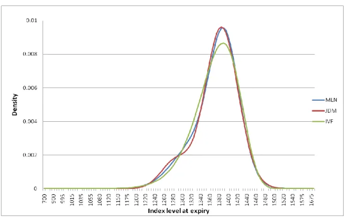
Fig. 1. Three risk-neutral densities on April 19, 2008
The graph of the RNDs (Figure 1) is in accordance with the statistical properties. The blue, red and green lines represent the mixture of two lognormals, the jump diffusion and implied volatility function densities respectively. The means of three densities are quite similar, and all the distributions are left-skewed. In addition, it is obvious that the left tails of all three densities are quite different. The jump diffusion model density reflects the small jump at around 1270. Moreover, the green line (the implied volatility function density) is higher than the other two lines in the range between 1290 and 1340, which indicates more probabilities in the left tails of implied volatility function density.
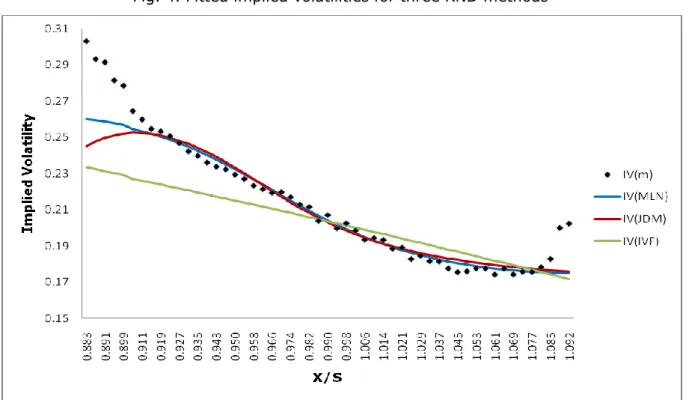
Figure 2 displays the implied volatilities for the market prices and for the three RND methods, against strike prices/index level. The black dots are the market implied volatilities. All three methods seem to fit the market implied volatilities well in the range 0.94 to 1.064, except for the strike prices furthest from the index level. The curves of mixture of two lognormals model and the jump diffusion model are almost identical, with slightly different from the curve of implied volatility function model.
5.3.2 RND on September 20, 2008 (crisis period)
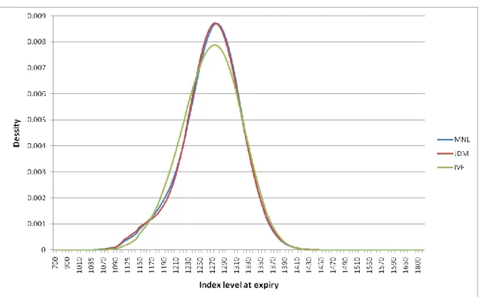
Table 4 describes the statistics on September 20, 2008 (during crisis period). The first and second moments of all three methods are similar (mean: around 1267; standard deviation: around 51). The actual closing index level was 1255.08, which is much lower than the expected value of three densities. The skewness and the kurtosis of both MLN and JDM densities are similar, while there are significant differences between these two densities and IVF density. The skewness of IVF density is negative 0.17 and the kurtosis is around 3, while the skewness and kurtosis of the other two densities are about -0.4 and 3.6. It indicates that the IVF density is closer to the lognormal distribution. Figure 3 and 4 show the estimated risk-neutral
densities and implied volatilities. The mixtures of two lognormals and jump diffusion model densities are similar, and both approaches provide a much better fit to the observed implied volatilities than implied volatility function method.
Table 4
Moments of the risk-neutral density on September 20, 2008
Index statistics MLN JDM IVF
Mean 1267.15337 1267.002407 1267.467182
Standard deviation 51.29110414 51.38879061 50.543684
Skewness -0.429984358 -0.407017392 -0.170059229
Kurtosis 3.605457088 3.572188562 3.031447945
Fig. 4. Fitted implied volatilities for three RND methods
5.3.3 RND on April 18, 2009 (post-crisis period)
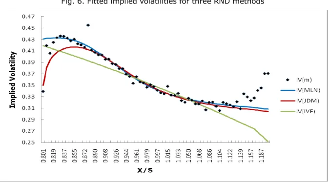
Table 5 summarizes the four moments of risk-neutral densities on April 18, 2009 (post-crisis period). The means of all three densities are similar, but are much smaller than the actual closing index level (869.6) on the expiration date. The standard deviations of both MLN and JDM densities are around 58.7, which are slightly higher than the IVF density standard deviation (58.01). In addition, all the skewnesses are negative, and there are no significant differences among different methods. However, the kurtosis of IVF density is close to 3, which is much smaller than the other two densities (around 3.35). The corresponding graphs (Figure 5 and 6) corroborate the results. The plotted densities of MLN and JDM are similar, but the mixture of two lognormals method provides a more satisfactory fit to the market implied volatilities. The IVF density differs in the left tail and is less leptokurtic than the other two densities. Additionally, the implied volatilities of the implied volatility function method do not present a close match with the market implied volatilities.
Table 5 Moments of the risk-neutral density on April 18, 2009
Index statistics MLN JDM IVF
Mean 842.6190408 842.5089833 842.4318802
Standard deviation 58.7496196 58.78701825 58.01389372
Skewness -0.327279176 -0.335798963 -0.290029973
Kurtosis 3.428589239 3.334620237 3.009977911
Fig. 5. Three risk-neutral densities on April 18, 2009
To sum up, in terms of the expected value, all three methods provide quite similar results. During the pre-crisis and post-crisis period, the mean values are smaller than the actual closing index level. It indicates that investors‘ expectations about index level are conservative. However, during the crisis period, the expected value is larger than the actual index level, which suggests that investors expect the better performance of the market. Moreover, the standard deviations of three methods are close to each other and they keep rising from pre-crisis to post-crisis period. The increasing volatility implies the increasing uncertainty about the index level movements. Furthermore, during the pre-crisis, both the skewness and kurtosis of three densities are similar, while during the crisis period and post-crisis period, the IVF density is close to the lognormal distribution with less skewed and less excess kurtosis. Finally, the MLN and JDM densities are almost identical during different periods, and they are slightly less skewed from pre-crisis to post-crisis period, with average from -0.6 to -0.3. The negative skewness appears to reflect the possibility of the major crash, and the levels of crash anxiety are more pessimistic during pre-crisis period than that during post-crisis period (Liu et al, 2007).
5.4 Parameter estimates of the jump diffusion model
Since the parameters of both mixtures of two lognormal models and implied volatility function models have no obvious economic meanings, the study tends to focus on the parameter explanations of jump diffusion models only.
The parameter estimates for the jump diffusion model are presented in Table 6. First of all, it is obvious that the volatility increases from 0.13 (pre-crisis), 0.16 (during crisis) to 0.29 (post-crisis). It indicates that the investors believe in a greater uncertainty about the price movements after the financial crisis. Moreover, the sign of parameter k are all negative, which suggests that the prices will jump down rather than jumping up. On April 19,
2008 (during pre-crisis period), the probability that a jump will occur before maturity (λT) is around 14%. This highest probability implies that the investors believe in a great likelihood of a jump occurrence. On April 18, 2009 (during post-crisis period), the probability drops to about 10%. Although the probability of jump occurrence during post-crisis period is lower than that of during pre-crisis period, the market seems still unstable. Finally, turning to the expected jump size (absolute value of λk), all the statistics on three dates are high. This means that investors expect a large jump down about the index level. In general, after the crisis, the market seems more unstable than before the crisis. And if the jump occurs after the crisis, the jump size will be much larger than that of pre-crisis period. Additionally, the pre-crisis period has the largest probability of jump occurrence. It seems to predict the crisis effectively.
Table 6
Estimates of the Bernoulli version of the jump diffusion model
19/04/2008 20/09/2008 18/04/2009 σ 0.129139492 0.164156368 0.287171979 λ 3.62039109 2.246470913 2.536477879 k -0.070229363 -0.083934557 -0.130082411 λT 0.143666313 0.089145671 0.100653884 Absolute value λk 0.254257759 0.188556542 0.329951157
Section VI Empirical results of Real World Density
Since the jump diffusion model assumes a different price process, and the additional flexibility of the implied volatility function appears to be not preferable for our data, the paper will focus the discussion only on the risk preference adjustments of mixtures of two lognormal densities.
Both the power utility function and beta function are used to transform MLN densities into real world densities. Meanwhile, the total 24 non-overlapping densities are divided into two sets (Year 2008 and Year 2009) to estimate risk parameters γ, and . The non-overlapping structure ensures the calculation of the likelihood function in (31 & 32), and the closing index levels (St*) on option expiry days t* are used. Firstly, the risk parameter of power utility function transformation will be discussed. Secondly, the parameter estimates of beta function transformation will be explained. Then, the likelihood-ratio test is used to test whether risk premium exists. Fourthly, the study will compare the RNDs and real world densities for two specific dates respectively (19/04/2008 and 18/04/2009). Finally, the moments of risk-neutral densities and real world densities will be compared.
6.1 Parameter estimation of power utility function transformation Table 1
Parameter estimates of power utility function transformation
γ annualized σ Risk premium
2008 -4.498559138 0.168262913 -0.756940664
2009 3.389965468 0.074343322 0.252021293
Table 1 presents the risk parameters for both Year 2008 and Year 2009 using the power utility function transformation. For the Year 2008, the constant
risk aversion parameter γ is negative (about -4.5), which appears irrational comparing with the results in other studies shown in Table 2. However, unlike the results of Mehra & Prescott (1985) and Cochrane & Hansen (1992), there is no evidence of the extreme in our results.
Table 2
Estimation of the coefficient of relative risk-aversion from previous studies
Study CRRA Range
Arrow (1971) 1
Friend and Blume (1975) 2
Hansen and Singleton (1982, 1984) -1.6-1.3
Mehra and Prescott (1985) 55
Ferson and Constantinides (1991) 0-12
Cochran and Hansen (1992) 40-50
Jorion and Giovannini (1993) 5.4-11.9
Bartunek and Chowdhury (1997) 0.2-0.6
Normandin and St-Amour (1998) <3
Aït-Sahalia and Lo (2000)a 12.7
Jackwerth (2000)b -15-20
Guo and Whitelaw (2001) 3.52
Note: This table is an update version of Pérignon & Villa (2002) Table 2 and Bliss & Panigirtzoglou (2004) Table VII. (a) The study by Aït-Sahalia and Lo (2000) does not assume constant risk aversion and 12.7 reported is an average value. (b) Jackwerth (2000) estimates absolute risk-aversion functions.
There are three potential explanations for the negative sign of CRRA. First of all, according to Taylor (2005) and Jackwerth (2000), some options are mispriced during the crisis period. These mispriced options reflect the anxiety about market crashes, which results in the negative risk parameter
γ (Taylor, ibid). In addition, Bliss & Panigirtzoglou (2004) consider that the risk aversion of the representative investor is volatility-dependent. During the crisis period, the volatility is high (annualized volatility of 2008 equals to 16.83%). More and more risk-averse investors leave the market to avoid further losses. As a result, the average level of risk aversion amongst the remaining investors decreases, and ultimately turns to the negative value. The final possible explanation is that investors are pessimistic rather than risk averse. It is difficult to distinguish between individual pessimism and risk aversion (Mansour, et al, 2008). Therefore, the negative γ may be a reflection of investors‘ pessimism about the market during the crisis rather than risk aversion. Moreover, the negative CRRA parameter in 2008 results in the negative risk premium as well. It makes sense that during the crisis period when investors are quite uncertain about the market, they may be willing to pay extras to ensure the minimum losses.
For the Year 2009, the CRRA parameter equals to 3.39. The result appears reasonable and accords well with those studies reported in Table 2. Although the annualized volatility decreased from 16.8% in 2008 to 7.4% in 2009, investors are still uncertain about the market, and hence require a high risk premium about 25.2%.
6.2 Parameter estimates of beta function transformation Table 3
Parameter estimates of calibration beta function transformation
α β
2008 1 1
The parameter estimates of calibration beta function transformation are presented in Table 3. A necessary and sufficient condition to have the risk-aversion property is ≤ 1 ≤ , with ≠ (Liu et al, 2007; Taylor, 2005). When this risk-aversion constraint is applied, both parameter and are equal to 1 for both years. The results indicate that there is no risk premium, and representative investors are risk-neutral, neither risk-seekers nor risk-aversion. However, they are inconsistent with the results obtaining from the power utility function transformation.
6.3 The likelihood-ratio test
Since the parameter estimates of two transformation methods are inconsistent, the likelihood-ratio test is used to test whether there is no risk premium during both periods. The null hypothesis is that the constant risk aversion parameter γ is equal to zero (H0: γ=0). The differences between the values of the log-likelihood function for the null hypothesis and alternative hypothesis will be multiplied by 2, and compared with chi-square distribution. The degree of freedom is one, because the alternative hypothesis has one more parameter than the null.
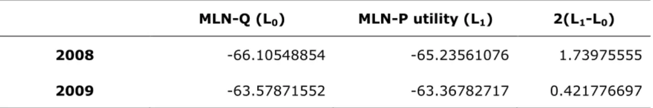
Table 4 summarizes the value of log-likelihood of both risk-neutral densities and real world densities. L0 represents the log-likelihood of null hypothesis that there is no risk premium, and L1 is the maximum value of log-likelihood for power utility function transformation.
Table 4
Values of log-likelihood for both H0 and H1
MLN-Q (L0) MLN-P utility (L1) 2(L1-L0)
2008 -66.10548854 -65.23561076 1.73975555
In terms of Year 2008, the value of 2(L1-L0) is around 1.74. The 10% critical point of 12 is 2.71, which is larger than 1.74. Therefore, the null hypothesis that there is no risk premium (γ=0) is accepted. For the Year 2009, the difference of two log-likelihoods is equal to 0.422, which is much smaller than the 10% critical point of 12. As a result, the null hypothesis is also accepted for the Year 2009.
Generally, although two different transformation methods appear to give contradictory results, the null hypothesis that there is no risk premium cannot be rejected for both years. Consequently, the parameter estimates for both power utility function and beta function methods seem to be acceptable.
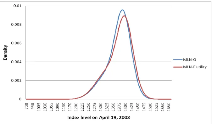
6.4 Comparison of risk-neutral densities and real world densities The real world densities of 19/04/2008 and 18/04/2009 are plotted to compare with the risk-neutral densities (Figure 1 and Figure 2), and Table 5 and 6 illustrate the four moments of both densities for two dates.
Table 5
Four moments of both densities on April 19, 2008
Index statistics MLN-Q MLN-P utility
Mean 1372.910005 1375.543812
Standard deviation 49.00588964 52.18352543
Skewness -0.619025371 -0.586809643
Kurtosis 3.483652643 3.217812219
For the first date, Table 5 summarizes the results. Compared with the risk-neutral density, the transformation increases the mean and standard deviation, while reduces both the skewness and kurtosis. The differences of
all four moments are not substantial. The corresponding graph (Figure 1) shows clearly that the real world density is less skewed and less leptokurtic.
Fig. 1. RND & real world density on April 19, 2008
Table 6
Four moments of both densities on April 18, 2009
Index statistics MLN-Q MLN-P utility
Mean 842.6190408 837.9707
Standard deviation 58.7496196 55.29025
Skewness -0.327279176 -0.2276
Kurtosis 3.428589239 3.483817
Table 6 summarizes the moments of both densities on April 18, 2009. After the transformation, both mean and standard deviation decrease. The skewnesses of both densities are negative, while the skewness of real world density is closer to 0. In addition, the kurtosis of real world density increases, but only changes slightly. The corresponding graph (Figure 2) corroborates
the findings as well.
Fig.2. RND & real world density on April 18, 2009
6.5 Comparison of the moments for RNDs and real world densities In order to further compare the risk-neutral densities and real world densities, the four moments of both densities are examined. Since the calibration transformation results show that the representative agent is risk-neutral, the study will only compare the risk-neutral densities with real world densities transforming through the power utility function. Table 6 summarizes the mean, standard deviation, skewness and kurtosis of 24 densities in total. The mean and standard deviation are divided by the actual closing index prices on expiration dates (St*).
Table 6
Moments for RNDs and real world densities
Index Statistics MLN-Q MLN-P utility
Mean/St* Minimum 0.877093957 0.883099347 Maximum 1.16092831 1.125055155 Mean 1.011513718 0.99272785 Standard deviation 0.069131416 0.056024345 Standard deviation/St* Minimum 0.027212265 0.027870486 Maximum 0.124133775 0.220856854 Mean 0.055968242 0.059524848 Standard deviation 0.026302562 0.04167562 Skewness Minimum -2.262780521 -0.946845477 Maximum 0.272924613 0.547962319 Mean -0.538915892 -0.283186531 Standard deviation 0.552583581 0.376975727 Kurtosis Minimum 2.308896023 1.741988901 hMaximum 19.37108742 14.52367034 Mean 4.577364831 3.965778566 Standard deviation 3.599823024 2.596996338
The RNDs and their transformations have similar average expected values, and means of both densities are close to the closing index levels on expiration dates. In addition, the real world densities have slightly higher average standard deviations than the averages of the RNDs. It is interesting that all the real world densities in 2008 have higher average standard
deviations than the averages for the RNDs, while they all have lower average standard deviations in 2009. It is possible that the negative sign of CRRA parameter in 2008 results in the increase in the standard deviation of the real world densities. Moreover, most of the densities have negative skewness. The real world densities obtained by transformations are less negatively skewed with average -0.28 than the risk-neutral densities (-0.54). Similar to the skewness, the real world densities are also less leptokurtic than the risk-neutral densities. Overall, the risk adjustments change the RNDs to make them more like the lognormal distribution, with skewness closer to one and less excess kurtosis. However, in terms of all four moments, the differences between risk-neutral densities and real world densities are not substantial, which is also be corroborated by log-likelihood test.