Mean-variance relation: a sentimental affair.
RUI ASCENSO 152412028
ABSTRACT
This work documents the role investor sentiment plays on the market’s mean-variance tradeoff. We find that, during high-sentiment periods, investor sentiment undermines an otherwise positive mean-variance tradeoff. In low-sentiment periods, the common understanding holds that investors should obtain a compensation for bearing variance risk. These findings are robust to different stock return indices, variances estimates and sentiment measures. We also provide international evidence for five other countries and point out a possible leading role for U.S. sentiment.
Professor José Faias Supervisor
Dissertation submitted in partial fulfillment of requirements for the degree of International Master of Science in Finance, at Universidade Católica Portuguesa, September 2015.
i
Acknowledgments
I am exceptionally grateful to Professor José Faias for his never-ending guidance, patience and care throughout the period we have met, and in particular throughout the completion of my dissertation. I thank him as well for the research fellowship opportunity last summer, a rewarding experience that ultimately represented a great contribution to this work.
I thank Católica-Lisbon School of Business and Economics for providing work facilities, access to databases, subscription to academic literature and 24-hour per day availability. I thank Carnegie Mellon University for it all started there, from the initial idea to be developed in this dissertation, to the first stages in collecting literature and data. I acknowledge “Fundação para a Ciência e Tecnologia” for financial support under the project PTDC/EGE-GES/120282/2010. I also thank Malcolm Baker, Jeff Wurgler and Yu Yuan for providing the investor sentiment data and encouraging the realization of this work, and the Wharton Research Data Services (WRDS) for the support resources and data provided. I am grateful to my father for suggesting the title of this dissertation.
Several people I have met shall not live unknown, as their importance in my life and their support during this challenging time is far beyond from what I can thank for. I name them as they like to be called and in undistinguished order: Pasha, Cravo, Max, Tigas, França, Rustam, Alexey, João, Pipa, Elvas, Henrique and obviously, Afonso and Manelão. I am, in part, them; this work is, in part, theirs. And then, there is Her. Because my sun rises and sets with Her, and because that is enough, always and evermore. This work is devoted to Her.
Above all, I dedicate this work to my parents, my godparents and my sister. They are my family, and to family no words are required. I love them and hope they can be proud of what I was able to achieve here.
ii
Table of Contents
I. Introduction ... 1
II. Data and descriptive statistics ... 6
III. Empirical results ... 14
IV. Robustness checks ... 19
iii
Index of Tables
Table 1. Descriptive statistics of monthly stock returns and conditional variances ... 13
Table 2. Excess returns against conditional variance in rolling window model ... 16
Table 3. Excess returns against conditional variance in GARCH (1,1) ... 18
Table 4. Excess returns against conditional variance in rolling window model ... 21
Table 5. Excess returns against conditional variance in GARCH (1,1) ... 22
Table 6. S&P 500, DJIA and Nasdaq 100 excess returns against conditional variance in the rolling window model ... 23
Table 7. S&P 500, DJIA and Nasdaq 100 excess returns against conditional variance in GARCH (1,1) ... 24
Table 8. International excess returns against conditional variance in rolling window model . 26 Table 9. Excess returns against conditional variance in rolling window model for macro-variables two-regime periods ... 28
Table 10. Excess returns against conditional variance in asymmetric GARCH (1,1) ... 29
Index of Figures Figure 1. Realized variance and GARCH variance, 1965-2010. ... 7
Figure 2. BW and MCSI investor sentiment indices, 1965-2010. ... 10
1 "I'll play it first, and tell you what it is later."
- Miles Davis
I. Introduction
Ever since Markowitz’s seminal work of the 1950s, a tremendous body of finance theory and empirical evidence has been developed over the relation between the return on an asset and the notion of variance, aiming to solve a dilemma each investor faces: the opposing objectives of high return versus low risk. 1 As Ghysels et al. (2005) put it, the
risk-return tradeoff is so fundamental in financial economics that it could be described as “the first fundamental law of finance”. In a recent study, Yu and Yuan (2011, YY hereafter) find that the sentiment index in Baker and Wurgler (2006, BW henceforth) significantly affects the U.S. mean-variance tradeoff. This dissertation builds on both the mean-variance and sentiment literature, to ultimately document the impact investor sentiment has on the mean-variance tradeoff, and provide significant international evidence, in a clear attempt to contribute to the existing literature with a more integrated and comprehensive work on the link between sentiment, risk and return.
We revisit the risk-return tradeoff to investigate whether investor sentiment disturbs this relation. We find investor sentiment to play an indisputable part on the mean-variance relation: our results suggest that sentiment is likely to weaken the connection between the conditional mean and variance of returns. The premise of a positive mean-variance tradeoff holds when market sentiment is low, but fades away in periods of high sentiment. Our results seem consistent with sentiment literature. High-sentiment periods account for greater presence of sentiment traders in the market. The greater presence of these
1 Harry Markowitz was awarded the 1990 Nobel Prize in Economics for having developed the theory of portfolio choice, published in an essay entitled "Portfolio Selection".
2 oriented traders can move prices away from rational levels and undermine the expected positive mean-variance relation.
Theories of rational asset pricing often suggest a positive relation between the market’s expected return and variance [Merton (1973, 1980)].2 Yet the tradeoff has been hard to find
in the data and numerous studies find rather mixed empirical evidence on the mean-variance relation. Goyal and Santa-Clara (2003), Ghysels et al. (2005), Guo and Whitelaw (2006), Brandt and Wang (2007), Lundblad (2007), and Pastor et al. (2008) find a positive and significant relation between the conditional variance and the conditional mean of the stock market return. French et al. (1987), Baillie and DeGennaro (1990) and Campbell and Hentschel (1992) also find a positive although frequently insignificant relation. Contrarily, Campbell (1987), Nelson (1991), Whitelaw (1994), Lettau and Ludvigson (2003), and Brandt and Kang (2004) find a significantly negative relation. Turner et al. (1989), Glosten et al. (1993), Harvey (2001), and MacKinlay and Park (2004) find both a positive and a negative relation depending on the method used.3 In fact, the results seem highly sensitive to
methodology as the conclusions on the mean-variance relation proved to be greatly influenced by the conditional variance models selected, and thus the evidence we find in the literature is still inconclusive.4
More recently, behaviorists’ theories, departing from rational asset pricing, recurrently consider the influence of investor sentiment. BW (2007) define investor sentiment broadly as “a belief about future cash flows and investment risks that is not justified by the facts at hand”. Whilst classical finance theory leaves no role for investment sentiment, the history of
2 However, Abel (1998), Backus and Gregpry (1993), and Gennotte and Marsh (1993) present models in which a negative relation between return and variance is consistent with equilibrium.
3 See also Pindyck (1984), and Chan et al. (1992).
4 However, YY (2011) show that after controlling for BW (2006) investor sentiment, the results are impressively robust across all the conditional variance models.
3 stock market is full of striking events in which a dramatic level or change in stock prices seems to defy explanation. And the standard finance model has presented considerable difficulty fitting many of these events. As a result, behaviorists have been working to enhance the standard model and present alternatives.
There is today a reasonable large and growing literature about investor sentiment, particularly fostered since BW (2006, 2007) developed a powerful sentimental index and predict that broad waves of sentiment will have greater effects on hard to arbitrage and hard to value stocks (e.g. small, young, high volatility, unprofitable, non-dividend-paying, extreme-growth and distressed stocks). Prior to BW sentiment index, De Long et al. (1990) present a model of an asset market in which irrational noise traders with erroneous stochastic beliefs affect prices and earn higher expected returns. Glushkov (2005) show that sentiment affects stocks of some firms more than others due to higher “sentiment beta”. Other papers have found evidence for a role of investor sentiment in U.S. stock market returns both in the short run [Simon and Wiggins (2001), Brown and Cliff (2004), Qiu and Welch (2004), Kaniel et al. (2006), Lemmon and Portniaguina (2006)], and in the long run [Brown and Cliff (2005) and Yuan (2005)].
The presence of sentiment investors, with both optimistic and pessimistic expectations about the market, is well documented [Lee et al. (1991), Ritter (1991), BW (2006, 2007) and Baker et al. (2012)] and its behavior on the financial markets may provide some useful context to our results. Empirical studies show that sentiment traders are unwilling to take short positions. Barber and Odean (2008) reveal that individual investors, who top the list of sentiment traders candidates, “are more likely to buy attention-grabbing stocks than to sell them” and document that short positions represent only 0.29% of all positions taken by these investors. Since sentiment traders are reluctant to short, they participate more intensely
4 and have a stronger influence in the equity market when the market is optimistic and sentiment is high, as they tend to purchase more stocks – other studies enhance this view [Karlsson et al. (2005) and Yuan (2008)]. The greater influence of such investors when sentiment is high perverts the mean-variance tradeoff. Moreover, sentiment traders are likely to be less sophisticated, inexperienced and naive investors and therefore they can misestimate variance. Sentiment investors are by definition less prepared than, say, institutional investors to understand how to accurately measure risk. This leads them to misestimate the variance of returns and consequently misrepresent risk, distorting the risk-return relation. These considerations directly support our results. The amplified presence and activity of sentiment-driven traders when aggregate market sentiment is high should challenge an otherwise positive mean-variance tradeoff in the stock market.
Not only in the academia have the influence of investor sentiment and the presence of sentiment traders been documented. Financial media reports more and more often the dynamics between sentiment and the financial markets in their headlines, and the industry tries to capture it in their strategies. [e.g. Financial Times on the last U.K. general election, April 2015 – “Doubt surrounding the forthcoming election is weighing on investor sentiment and increasing volatility in UK.”; Financial Times, November 2012 – “Italy’s government borrowing costs have fallen to lows not seen for more than two years, highlighting more positive investor sentiment towards the eurozone’s «periphery» economies.”; Financial Times on trading and the social media, March 2012 – “Some hedge funds have already begun trading strategies based on sentiment on Twitter, such as London-based Derwent Capital Markets. Researchers at the University of Indiana in 2009 also designed an algorithm assessing mood moves on Twitter that could predict a rise or fall in
5 the Dow Jones Industrial Average with 87 per cent accuracy three to four days beforehand.”.]
Our methodology first builds on Yu and Yuan (2011) hypothesis and expands their sample. We use BW (2006) sentiment index to identify high- and low-sentiment periods through 1965 to 2010. There is a statistically significant and economically important positive tradeoff over low-sentiment periods, whereas during high-sentiment periods, the mean-variance relation appears as substantially weaker and virtually flat. We then conduct the same analysis using another widely accepted measure of investor sentiment, the University of Michigan’s consumer sentiment index,and the same conclusions apply.
Following, we test different stock return indices as a proxy for the U.S. stock market returns, including the S&P 500 index, the Dow Jones Industrial Average index (DJIA), and the Nasdaq 100 index. Additionally, we investigate whether this sentimental affair between risk and return is observable in other stock markets, specifically for Canada, Germany, France, U.K., and Japan. We use the same U.S. sentiment proxies; our results vary considerably depending on the volatility model employed. Whilst for the rolling window model we show similar and equally strong evidence of the ability of investor sentiment to distinguish the two-pattern risk-return tradeoff, for GARCH-like models, the same conclusions do not hold.
Moreover, we examine if alternative variables other than sentiment yield similar two-pattern mean-variance outcomes, namely the interest rate, the term premium, the default premium, the dividend-price ratio, and the consumption surplus ratio defined in Campbell and Cochrane (1999). The results are unequivocal and show that such variables perform poorly when compared to investor sentiment.Lastly, we try an asymmetric GARCH (1,1) as
6 an alternative to the standard GARCH (1,1) model, and we conclude both approaches yield identical results.
Subsequent sections are organized as follows. Section II introduces the volatility models used and describes thoroughly all data and its descriptive statistics. Empirical results are reported in section III. Section IV accommodates the different robustness tests performed. Section V concludes this dissertation.
II. Data and descriptive statistics
In this section we detail the data we use. We first discuss the importance of accurately estimating volatility in our work and introduce the two types of volatility models tested: the rolling window model and the GARCH model. Subsequently, we introduce the investor sentiment proxies considered in the analysis and then discuss the data set used to compute stock market returns. Overall, we used roughly eight primary data sources to conduct this dissertation. We use primarily U.S. data, as the United States is widely considered the world’s bellwether market and we are constrained by the availability of international data regarding, for instance, the sentiment proxies. Yet, we use international data, if available, mainly to perform robustness tests.
A. Volatility models
The first model we employ is the rolling window (RW) model, which is widely accepted as a method to estimate the conditional variance (e.g. French, Schwert, and Stambaugh, 1987). This model uses the realized variance of the current month as the conditional variance for the next month’s return:
𝑉𝑎𝑟𝑡(𝑅𝑡+1) = 𝜎𝑡2 =22
𝑁𝑡∑ 𝑟𝑡−𝑑2
𝑁𝑡
𝑑=1
7 where rt−d is the demeaned daily return in month t (obtained by subtracting the within-month mean return from the daily raw return), the subscript 𝑁𝑡 is the number of
trading days in month t, and 22 is the approximate number of trading days in one month. The GARCH-family models are perhaps the most thoroughly studied volatility models in the literature and have been massively used in modeling the volatility of stock market returns [e.g. Bollerslev (1986) proposes the GARCH model based on the ARCH model developed by Engle (1982)].
The second volatility model we use in this dissertation is the GARCH (1,1). In this model the conditional variance is modeled as:
𝑉𝑎𝑟𝑡(𝑅𝑡+1) = 𝜔 + 𝛼1𝜀𝑡2 + 𝛽𝑉𝑎𝑟𝑡−1(𝑅𝑡), (2)
where Vart(Rt+1) is the conditional variance and 𝜀𝑡 is the residual, i.e., the difference
between the realized return and its conditional mean.
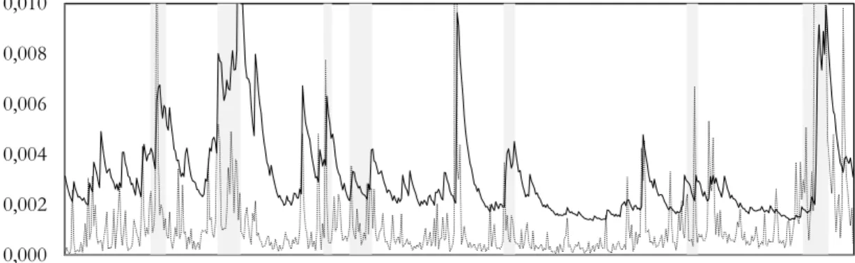
Figure 1 plots the monthly conditional variance for both the RW model and the GARCH model from 1965 to 2010.
Figure 1. Realized variance and GARCH variance, 1965-2010.
The figure presents the conditional variances estimated by the volatility models used, namely the rolling window model (dotted line) and the GARCH model (solid line). Due to sentiment data availability, we restrict our sample to the period from 1965 through 2010. Please refer to Table 1 for detail on variances’ descriptive statistics. Shaded areas denote periods designated recessions by the National Bureau of Economic Research.
0,000 0,002 0,004 0,006 0,008 0,010
8 In order to analyze to which extent investor sentiment is able to affect the standard tradeoff between expected returns and variance, it is as critical to accurately measure variance as it is to find representative proxies for sentiment and market returns.
B. Investor sentiment data set
Our sentiment data set is constrained by the availability of international sentiment proxies and cannot employ all those that the predominantly U.S. investor sentiment literature has examined. Yet, there are no definitive or uncontroversial measures. We measure investor sentiment using the Baker and Wurgler investor sentiment index as our main proxy of sentiment. We do use other proxies for investor sentiment as a robustness test, and find equally strong results.
i. Baker and Wurgler (BW) investor sentiment index
Our first investor sentiment measure is a monthly market-based sentiment series constructed by Baker and Wurgler (2006). The BW investor sentiment index is constructed based on the common variation in six underlying proxies for sentiment: the closed-end fund discount, NYSE share turnover, the number and average first-day returns on IPOs, the equity share in new issues, and the dividend premium. The authors form their composite index by taking the first principal component of these six proxies. The principal component analysis filters out idiosyncratic noise in the six measures and captures their common component: investor sentiment. To address concerns that each of these proxies for sentiment might contain common business cycle information, BW (2006) first regress each of the raw sentiment proxies on a set of macroeconomic variables and use the residuals to
9 build the sentiment index. 5 We obtain the sentiment data from Professor Jeff Wurgler’s
website. Due to sentiment data availability, we restrict our sample to the period from 1965 through 2010.
ii. University of Michigan’s consumer sentiment index (MCSI)
We use the monthly University of Michigan’s consumer sentiment index (henceforth, MCSI) as our second investor sentiment measure. The MCSI is based on the responses households give to the monthly Surveys of Consumers, telephone surveys that have been conducted at the University of Michigan since 1946, to gather information on consumer expectations regarding the overall economy. Consumer confidence indices have been broadly used as sentiment indicators in the literature. Carroll et al. (1994), Bram and Ludvigson (1998), and Ludvigson (2004) find that consumer sentiment indices forecast household consumption. Fisher and Statman (2003) and Lemmon and Portnaiguina (2006) relate the consumer confidence indices to security mispricing. Bergman and Roychowdhury (2008) investigate how firms adapt their disclosure policies strategically to investor sentiment. Schmeling (2009) examines whether consumer confidence affects expected stock returns internationally; and Beer et al. (2011) study the relation between investor sentiment and stock market crisis. As in the BW index, there are some concerns that the MCSI might reflect economic conditions instead of investor sentiment. To ease these concerns we regress the monthly index on the same six macroeconomic variables used by BW (2006). We create our yearly consumer sentiment index using the yearly averages of the residuals from this regression. We obtain the sentiment data from the University of Michigan Survey Research Center’s website. For comparison purposes, we restrict our sample to the period from 1965
5 The set includes the industrial production index growth, durable consumption growth, nondurable consumption growth, service consumption growth, employment growth, and a dummy variable for NBER recessions. More details can be found in the original paper at: http://people.stern.nyu.edu/jwurgler/.
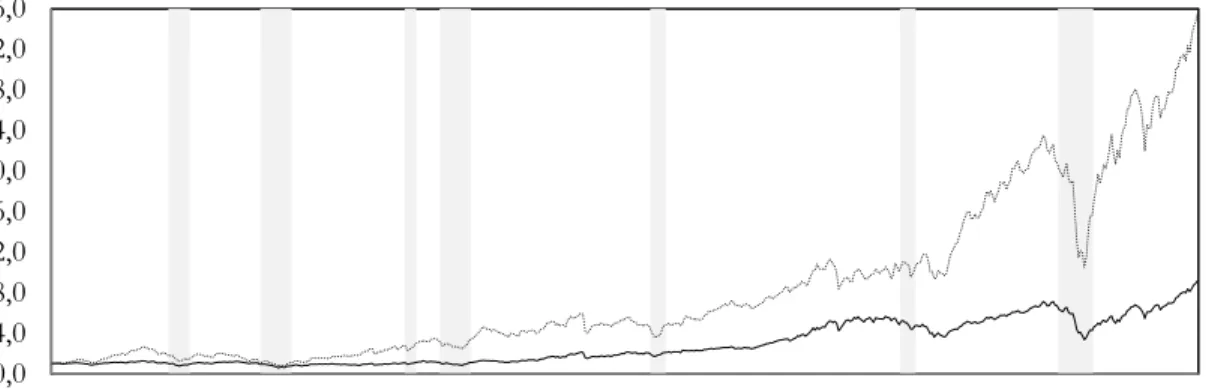
10 through 2010. Figure 2 plots BW and MCSI sentiment indices.
Figure 2. BW and MCSI investor sentiment indices, 1965-2010.
The figure presents the BW composite sentiment index (solid line) and the Michigan survey sentiment index (dotted line) from 1965 to 2010. BW index, a monthly market-based sentiment series, is the first principal component of six time-series proxies for sentiment. The first proxy is the year-end, value-weighted average discount on closed-end mutual funds; the second proxy is the NYSE detrended log share turnover; the third and fourth proxies are the annual number and the average annual first-day returns of initial public offerings; the fifth proxy is the equity share in new issues; and the sixth and last proxy is the dividend premium. MCSI index, a monthly survey-based sentiment series, is the result of the responses households give to the monthly Surveys of Consumers, telephone surveys that have been conducted at the University of Michigan since 1946, to gather information on consumer expectations regarding the overall economy. To control for macro-conditions, we regress both raw indices on the growth in industrial production, the growth in durable, nondurable, and services consumption, the growth in employment, and a flag for NBER recessions. Shaded areas denote periods designated recessions by the National Bureau of Economic Research.
BW index captures most of the empirically documented oscillations in investor sentiment. After the flash crash of 1962, also known as the Kennedy Slide, investor sentiment was low but picked up to reach a peak in the 1968 and 1969 electronic bubble. By the mid-1970s sentiment fell and went low but rose again to a subsequent peak in the biotech bubble of the late 1970s. Sentiment dropped in the late 1980s but recovered once more in the early 1990s, reaching its most recent peak in the Internet bubble. The stock market downturn of 2002 made sentiment fall again and kept it low through the early-2000s. The mid-2000s represented only a temporary recovery, since sentiment rose until 2006 but fell over again motivated by the 2007 and 2008 financial crisis. In the post-crisis period,
-30 -20 -10 0 10 20 30 -3 -2 -1 0 1 2 3 MC SI sen ti iment ind ex BW s en ti iment ind ex
11 investor sentiment went through a modest retrieval period and then remained approximately neutral until 2010. Our high-sentiment regime seems to be robust to what we find in the literature. Sentiment fluctuations have been previously studied by both empirical and academic work and are well documented in the academia. Malkiel (1990), Brown (1991), Siegel (1998), Shiller (2000), Cochrane (2003), and Ljunqvist and Wilhelm (2003), all provide evidence supporting our high-sentiment periods: the late 1960s, early and mid-1980s, and the mid and late-1990s.
Using the BW index, 22 years (47% of our sample period) are classified as high sentiment years; whilst the MCSI index divides the sample in 28 high- and 18 low-sentiment years. Our findings suggest the MCSI is a more optimistic measure than the BW index. Additionally, in the beginning of our sample, MCSI leaves the flash crash of 1962 behind sooner than the BW index, starting the sentiment series with a positive (optimistic) cycle, whereas the BW series is initiated with a negative (pessimistic) cycle. In the end of the sample period, also, the BW index seems more accurate in perceiving the increasing volatility prior to the financial crisis and predicting its arrival, with no clear positive or negative cycle and 3 negative years between 2002 and 2007. On the other hand, the MCSI shows no predictive power in this period, being positive between 2000 and 2008. Overall, the results corroborate the notion that the BW market-based measure is a considerably more accurate proxy of investor sentiment than the survey-based measure, the MCSI.
C. Stock market returns data set
We use the CRSP equal-weighted and value-weighted returns as proxies for U.S. stock market returns, and the one-month T-bill returns as the interest rate, both available on CRSP database. We use these data to compute equal-weighted and value-weighted excess market
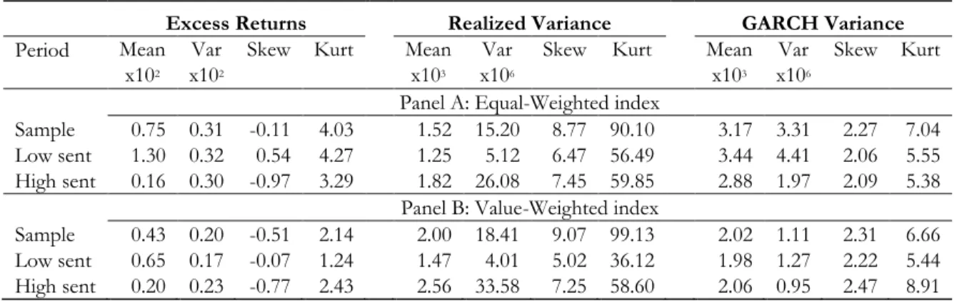
12 returns from January 1965 to December 2010, which is the sample period for which we have values of BW (2006) sentiment index. The results are based on a sample of monthly data, for a total of 552 end-of-the month observations. Figure 3 plots U.S. cumulative excess returns from 1965 to 2013.
Figure 3. U.S. equal-weighted and value-weighted cumulative excess returns, 1965-2013.
The figure presents U.S. equal- and value-weighted cumulative excess returns (dotted and solid lines, respectively) from 1965 to 2013. Both indices are constructed upon CRSP equal- and value-weighted returns, and the one-month T-bill returns, both available on CRSP database. Please refer to Table 1 for detail on returns’ descriptive statistics. Shaded areas denote periods designated recessions by the National Bureau of Economic Research.
The equal-weighted index has been extensively explored in the sentiment literature. Theory predicts that small firms will be most affected by sentiment, and hence value-weighting can obscure the relevant patterns. Contrarily, equal-weighted returns represent an excellent and accommodating stage to examine the effects of investor sentiment since they are more influenced by those small-cap stocks. Baker and Wurgler (2006) noticed that small stocks tend to be unprofitable and have extreme potential growth, which makes them more vulnerable to speculation, and thus extremely attractive to optimists and speculators. Additionally, small stocks are less exposed to arbitrage because of their high idiosyncratic risk (Wurgler and Zhuravskaya, 2002) and their high costs to short sell (Jones and Lamont, 2002). Higher idiosyncratic risk leads to particularly riskier relative-value arbitrage, whilst
0,0 4,0 8,0 12,0 16,0 20,0 24,0 28,0 32,0 36,0
13 high costs to sell constrain arbitrage strategies’ profits. The evidence found in this work supports the existing literature. However, we also examine the value-weighted index and we obtain equally strong results. The impact of sentiment on the mean-variance relation is robust across the entire stock data set.
In Table 1, we present the descriptive statistics of market excess returns, realized variance, and GHARCH variance. These statistics point out opposite patterns to both the low-sentiment and the high-sentiment regime, regardless of the index used.
Table 1. Descriptive statistics of monthly stock returns and conditional variances
The table contains summary statistics of monthly excess returns, monthly realized variance and monthly GARCH variance from January 1965 to December 2010. The excess returns are calculated using the returns on the NYSE-Amex index and the returns on the one-month T-bill. The realized variance is computed from the within-month daily returns. GARCH variance is estimated by the GARCH (1,1) model.
Excess Returns Realized Variance GARCH Variance
Period Mean Var Skew Kurt Mean Var Skew Kurt Mean Var Skew Kurt
x102 x102 x103 x106 x103 x106
Panel A: Equal-Weighted index
Sample 0.75 0.31 -0.11 4.03 1.52 15.20 8.77 90.10 3.17 3.31 2.27 7.04 Low sent 1.30 0.32 0.54 4.27 1.25 5.12 6.47 56.49 3.44 4.41 2.06 5.55 High sent 0.16 0.30 -0.97 3.29 1.82 26.08 7.45 59.85 2.88 1.97 2.09 5.38
Panel B: Value-Weighted index
Sample 0.43 0.20 -0.51 2.14 2.00 18.41 9.07 99.13 2.02 1.11 2.31 6.66 Low sent 0.65 0.17 -0.07 1.24 1.47 4.01 5.02 36.12 1.98 1.27 2.22 5.44 High sent 0.20 0.23 -0.77 2.43 2.56 33.58 7.25 58.60 2.06 0.95 2.47 8.91
In the low-sentiment regime, the mean of the equal-weighted returns is 1.30%, much higher than its equivalent in the high-sentiment period, which is only 0.16%. This evidence is also valid for the value-weighted returns, although the difference is smaller in that case. Sentiment literature corroborates this pattern, which is in accordance with the economic intuition that high sentiment raises the price and depresses the return.
The negative skewness of stock returns is much of an established fact in the financial literature. Yet, we report some insightful patterns on the role sentiment may play in the skewness of these returns (Table 1). Whilst in the high-sentiment periods, our returns sample substantiate the common idea of negatively skewed returns (-0.97 for the equal-weighted
14 index and -0.77 for the value-weighted index), in the low-sentiment regime the skewness of the returns are positive (0.54 in the equal-weighted index) or even close to zero (-0.07 in the value-weighted index).
According to our intuition, we expect conditional variance to be larger in the high-sentiment regime, subject to the fact that in high-high-sentiment periods stock prices are more affected by the presence of sentiment traders in the market than in low-sentiment periods. Table 1 confirms our argument for realized variance: the mean of realized variance, as well as all the remaining moments presented, are substantially higher in the high-sentiment periods, suggesting that prices are more volatile in these periods due to the great influence of sentiment traders. GARCH variance yields the same characteristics for the value-weighted index, but not for the equal-weighted index for which, with the exception of skewness, all GARCH variance moments are higher in low-sentiment periods, challenging our intuition.
III. Empirical results
In this section we relate investor sentiment, expected returns and variance, eager to understand whether and how sentiment influences the mean-variance tradeoff. We test the relation between the conditional mean and variance of returns free from investor sentiment interference in the equation:
𝑅𝑡+1 = 𝑎 + 𝑏𝑉𝑎𝑟𝑡(𝑅𝑡+1) + 𝜀𝑡+1, (3)
being 𝑅𝑡+1 the monthly excess return and 𝑉𝑎𝑟𝑡(𝑅𝑡+1) the conditional variance. To
investigate our claim that this relation is weakened in the high-sentiment periods, we study the following two-regime equation:
15 where we incorporated the dummy variable 𝐷𝑡 to account for the high-sentiment regime.
This means that 𝐷𝑡 equals one if month 𝑡 is comprised in a period of high sentiment in the
market and zero otherwise. High- and low-sentiment regimes are identified using the BW sentiment index: a certain year is classified as a high-sentiment year if the preceding year’s sentiment is positive; any month falling in a high-sentiment year is therefore classified as a high-sentiment month. In our 1965 to 2010 sample period, 22 out of the 46 years fall into the high-sentiment regime, being the low-sentiment regime constituted by the remaining 24 years. We expect negative 𝑏1+ 𝑏2 and positive 𝑏1. Because high sentiment should attenuate
the mean-variance tradeoff we expect 𝑏1+ 𝑏2 to be negative. Because sentiment traders are
barely noticed and have little impact during low-sentiment periods, investors should obtain positive compensation for bearing volatility and thus we expect 𝑏1 to be positive.
A. Mean–variance relation in Rolling Window model
The rolling window model is the first model we use to estimate variance. Table 2 reports the coefficients and test-statistics from the regressions with the rolling window model as the conditional variance model and the BW sentiment as the sentiment measure.
The mean-variance relation in the one-regime equation, 𝑏, is -0.39 with a t-statistic of -0.48, and the R2 of the regression is approximately 1%. These results suggest a weak and
rather inconclusive mean-variance tradeoff in the one-regime scenario. In contrast, the estimates from the two-regime equation clearly distinguish two different patterns in the mean-variance dynamics, supporting the idea that investor sentiment affects this relation. In the low-sentiment periods, we observe a significant and positive relation between variance and expected returns (𝑏1 is 4.28 with a t-statistic of 3.18), while in the high-sentiment periods
16 Additionally, the two-regime equation has more descriptive ability than the one-regime equation, as R2 increases from 1% to 3%.
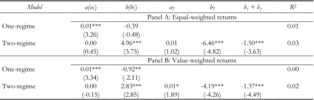
Table 2. Excess returns against conditional variance in rolling window model
The table reports the estimates and t-statistics of the rolling window model regressions in BW sentiment regimes: 𝑅𝑡+1 = 𝑎 + 𝑏𝑉𝑎𝑟𝑡(𝑅𝑡+1) + 𝜀𝑡+1, (3) 𝑅𝑡+1 = 𝑎1+ 𝑏1𝑉𝑎𝑟𝑡(𝑅𝑡+1) + 𝑎2𝐷𝑡+ 𝑏2𝐷𝑡𝑉𝑎𝑟𝑡(𝑅𝑡+1) + 𝜀𝑡+1, (4) 𝑉𝑎𝑟𝑡(𝑅𝑡+1) = 22 ∑ 𝑁1 𝑡 𝑁𝑡 𝑑=1 𝑟𝑡−𝑑2 , (1)
Rt + 1 is the monthly excess return on the NYSE-Amex index. Vart(Rt + 1) is the conditional variance. Dt is the
dummy variable for BW high-sentiment periods. rt-d is the daily demeaned NYSE-Amex index return (the daily
return minus the within-month mean). Nt is the number of trading days in month t, and 22 is the approximate
number of days in one month. Sample period is January 1965 to December 2010. The numbers in parentheses are t-statistics from the Newey-West standard error estimator. ***, **, * denote a 1%, 5% and 10% significance levels of the t-statistics, respectively.
Model a(a1) b(b1) a2 b2 b1 + b2 R2
Panel A: Equal-weighted returns
One-regime 0.01*** -0.39 0.01
(3.26) (-0.48)
Two-regime 0.01** 4.28*** 0.00 -5.54*** -1.26*** 0.03
(2.04) (3.18) (-0.74) (-4.05) (-2.91)
Panel B: Value-weighted returns
One-regime 0.01*** -0.92** 0.00
(3.34) (-2.11)
Two-regime 0.00 2.46** 0.00 -3.75*** -1.29*** 0.02
(1.33) (2.39) (0.43) (-3.62) (-4.16)
In Panel B, we present similar results regarding the value-weighted returns. During low-sentiment periods the mean-variance tradeoff is 2.46 with a t-statistic of 2.39 and during high-sentiment periods the relation is -1.29 with t-statistic of -4.16. Again, the two-regime equation has more descriptive ability than the one-regime equation (higher R2). These results
corroborate YY(2011) main hypothesis, in which we built upon to develop our work: investor sentiment seems to affect the mean-variance dynamics of the market, compromising an otherwise positive tradeoff when sentiment is high.
The fact that we observe similar patterns with the value-weighted returns suggests that investor sentiment’s impact on the relation between variance and returns is also present on large-cap stocks, although its influence is stronger in small-cap stocks. This is consistent
17 with the literature. Glushkov (2005) shows that sentiment affects stocks of some firms more than others due to higher “sentiment beta”. BW (2007) predict that broad waves of sentiment will have greater effects on hard to arbitrage and hard to value stocks such as small, young, high volatility, unprofitable, non-dividend-paying, extreme-growth and distressed stocks.
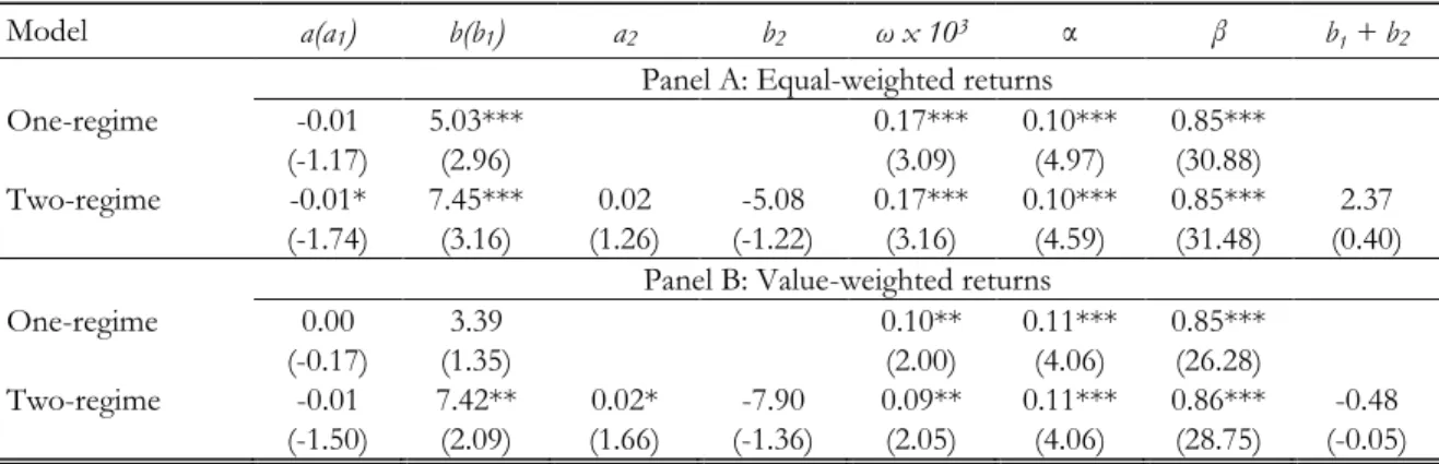
B. Mean–variance relation in GARCH (1,1) model
Tables 3 reports the estimates and test-statistics from the regressions with the GARCH (1,1) as the conditional variance model. BW investor sentiment is the sentiment measure used.
Under the one-regime setting, the mean-variance relation, 𝑏, is positive and statistically significant for the GARCH model (𝑏 is 5.03 with a t-statistic of 2.96), which opposes to the relation we find with the rolling window model. Under the two-regime setting, again, we find different two-pattern evidence when compared with the rolling window model: although in low-sentiment periods, there is the same strong and statistically significant positive tradeoff between the mean and the variance of returns expressed in the coefficient 𝑏1 (𝑏1 is 5.55 with
a t-statistic of 2.74), during high-sentiment we find a positive but weak, non-significant tradeoff (𝑏1+ 𝑏2 is 3.90 with a t-statistic of 0.72). In fact, the mean-variance slope, 𝑏1+ 𝑏2,
is never significantly positive for our estimates, regardless of using equal- or value-weighted returns.
Being nearly flat in all other cases, the mean-variance slope is only significantly negative if we choose the rolling window model as the conditional variance model (𝑏1+ 𝑏2
is -1.26 with a t-statistic of -2.91 with equal-weighted returns, and equal to -1.29 with a t-statistic of -4.16 with value-weighted returns, as reported in Table 2). Thus, whilst both our
18 models suggest that sentiment influences the risk-return relation by distinguishing two different patterns where the positive relation is, at least, challenged, only the rolling window model captures with statistical and economic significance the impact of investor sentiment. Table 3. Excess returns against conditional variance in GARCH (1,1)
The table reports the estimates and t-statistics of the GARCH (1,1) model regressions in BW sentiment regimes:
𝑅𝑡+1 = 𝑎 + 𝑏𝑉𝑎𝑟𝑡(𝑅𝑡+1) + 𝜀𝑡+1, (3)
𝑅𝑡+1 = 𝑎1+ 𝑏1𝑉𝑎𝑟𝑡(𝑅𝑡+1) + 𝑎2𝐷𝑡+ 𝑏2𝐷𝑡𝑉𝑎𝑟𝑡(𝑅𝑡+1) + 𝜀𝑡+1, (4)
𝑉𝑎𝑟𝑡(𝑅𝑡+1) = 𝜔 + 𝛼1𝜀𝑡2+ 𝛽𝑉𝑎𝑟𝑡−1(𝑅𝑡), (2)
Rt + 1 is the monthly excess return on the NYSE-Amex index. Vart(Rt + 1) is the conditional variance. Dt is the
dummy variable for BW high-sentiment periods. Sample period is January 1965 to December 2010. The numbers in parentheses are t-statistics from the Newey-West standard error estimator. ***, **, * denote a 1%, 5% and 10% significance levels of the t-statistics, respectively.
Model a(a1) b(b1) a2 b2 ω x 103 α β b1 + b2
Panel A: Equal-weighted returns
One-regime -0.01 5.03*** 0.17*** 0.10*** 0.85*** (-1.17) (2.96) (3.09) (4.97) (30.88)
Two-regime 0.00 5.55*** -0.01 -1.65 0.17*** 0.10*** 0.85*** 3.90 (-0.39) (2.74) (-0.47) (-0.41) (3.00) (4.41) (28.66) (0.72)
Panel B: Value-weighted returns
One-regime 0.00 3.39 0.10** 0.11*** 0.85***
(-0.17) (1.35) (2.00) (4.06) (26.28)
Two-regime 0.00 4.26** 0.00 -1.40 0.09** 0.11*** 0.85*** 2.86 (0.00) (2.13) (-0.28) (-0.27) (1.97) (3.97) (26.35) (0.37)
The literature has long reported conflicting conclusions dependent on the methodology, especially on the conditional variance models used. Our results, however, are not incompatible across the volatility models used, if in the two-regime setting: there is a strong, significant positive mean-variance tradeoff in low-sentiment periods, but little if any in high-sentiment periods. The influence of investor sentiment in such periods sabotages an otherwise positive relation between return and risk. Although in line with YY (2011) main findings, our results do not indicate the same level of robustness across volatility models proposed by YY (2011). We find the same empirical conclusions in the value-weighted returns, which indicates that the impact of sentiment in large-cap stocks must not be overlooked. Even though its impact is stronger in small-cap stocks, investor sentiment seems
19 to affect all stocks in our sample.
Furthermore, it is interesting to observe the predictive ability of the sentiment dummy (𝑎2). It is commonly believed that when investor sentiment is high (low), the stock market is
overvalued (undervalued). Then, as sentiment eventually returns to its long-run mean, we expect prices to commove with sentiment, and in result, we expect a lower (higher) future return. In our models, this intuition corresponds to the predictive ability of the sentiment dummy, 𝑎2, which is not significant in any of our estimates. According to our results, the
predictive ability of the sentiment dummy is faint at the one-month horizon. This finding corroborates YY (2011), and is consistent with Brown and Cliff (2005) and Yuan (2005) who show that sentiment’s long-run ability to predict market returns is stronger than in the short-run, due to sentiment’s high persistence.
IV. Robustness checks
This section reports the results of a range of robustness checks performed in this dissertation. We first examine whether the empirical results presented in the previous section hold for our alternative sentiment measure, MCSI, and alternative proxies of U.S. market returns. Following, we consider certain international evidence and study how investor sentiment influences the mean-variance tradeoff of five other stock markets. We also compare the performance of our sentiment measure to the one of several macro-economic variables. Lastly, we test a different GARCH-family model as an alternative to GARCH (1,1), namely the asymmetric GARCH (1,1). 6
6 The asymmetric GARCH (1,1) model was also employed to model volatility throughout all our work, including all robustness checks. The conclusions are of the same nature as the ones for the standard GARCH (1,1) model. We do not report them in this dissertation but they can be made available upon request.
20 A. U.S. market evidence
i. Using alternative investor sentiment proxies
In Section III we identify the prominent role of investor sentiment in the mean-variance dynamics, and use BW sentiment index as a proxy for sentiment. To use an accurate sentiment proxy is understandably a critical factor in our work. We perform the same analysis presented in Section III using the MCSI index, described in Section II. Tables 4 and 5 report the estimates and test-statistics from the regressions with the rolling window and the GARCH (1,1) as the conditional variance models, respectively, and MCSI as the sentiment proxy. 7
Under the one-regime setting, all the estimates and test-statistics from the regressions are equal to the ones from the BW sentiment regressions, since investor sentiment is not taken into account in this scenario. Therefore under this sentiment-free setting the mean-variance relation, 𝑏, is positive and statistically significant for the GARCH (1,1), but negative and non-significant for the rolling window model. Under the two-regime setting, the rolling window model yields the same two-pattern evidence that we find with the BW index: in low-sentiment periods, there is a strong and statistically significant positive tradeoff between the mean and the variance of returns expressed in the coefficient 𝑏1 (𝑏1 is 4.96 with a t-statistic
of 3.75 and 7.45 with a t-statistic of 3.16 in the rolling window and in the standard GARCH, respectively), whereas during high-sentiment we find strong and statistically significant negative tradeoff with the rolling window but no significant relation with the GARCH (1,1) (𝑏1+ 𝑏2 is -1.50 with a t-statistic of -3.63 and 2.37 with a t-statistic of 0.40 in the rolling
7 Although we only present the sample period from January 1965 to December 2010 in Tables 4 and 5, we extended our sample for this particularly robustness check up to December 2014, since we do not face the same data availability constraints as with BW sentiment. The conclusions are of the same nature and can be made available upon request.
21 window and in the GARCH models, respectively). The predictive ability of the sentiment dummy (𝑎2) reveals to be faint at the one-month horizon, once again.
Table 4. Excess returns against conditional variance in rolling window model
The table reports the estimates and t-statistics of the rolling window model regressions in MCSI sentiment regimes: 𝑅𝑡+1 = 𝑎 + 𝑏𝑉𝑎𝑟𝑡(𝑅𝑡+1) + 𝜀𝑡+1, (3) 𝑅𝑡+1 = 𝑎1+ 𝑏1𝑉𝑎𝑟𝑡(𝑅𝑡+1) + 𝑎2𝐷𝑡+ 𝑏2𝐷𝑡𝑉𝑎𝑟𝑡(𝑅𝑡+1) + 𝜀𝑡+1, (4) 𝑉𝑎𝑟𝑡(𝑅𝑡+1) = 22 ∑ 𝑁1 𝑡 𝑁𝑡 𝑑=1 𝑟𝑡−𝑑2 , (1)
Rt + 1 is the monthly excess return on the NYSE-Amex index. Vart(Rt + 1) is the conditional variance. Dt is the
dummy variable for MCSI high-sentiment periods. rt-d is the daily demeaned NYSE-Amex index return (the
daily return minus the within-month mean). Nt is the number of trading days in month t, and 22 is the
approximate number of days in one month. Sample period is January 1965 to December 2010. The numbers in parentheses are t-statistics from the Newey-West standard error estimator. ***, **, * denote a 1%, 5% and 10% significance levels of the t-statistics, respectively.
Model a(a1) b(b1) a2 b2 b1 + b2 R2
Panel A: Equal-weighted returns
One-regime 0.01*** -0.39 0.01
(3.26) (-0.48)
Two-regime 0.00 4.96*** 0.01 -6.46*** -1.50*** 0.03
(0.45) (3.75) (1.02) (-4.82) (-3.63)
Panel B: Value-weighted returns
One-regime 0.01*** -0.92** 0.00
(3.34) (-2.11)
Two-regime 0.00 2.83*** 0.01* -4.19*** -1.37*** 0.02 (-0.15) (2.85) (1.89) (-4.26) (-4.49)
The importance of investor sentiment to fully understand the relation between the conditional mean and the conditional variance of stock returns is deeply supported by our results. To use a market-based series or, alternatively, a consumer confidence measure as a proxy of investor sentiment leads us virtually to the same set of conclusions: sentiment distorts a tradeoff that would otherwise translate a positive and statistically significant relation between the return and risk of stock markets.
22 Table 5. Excess returns against conditional variance in GARCH (1,1)
The table reports the estimates and t-statistics of the GARCH (1,1) model regressions in MCSI sentiment regimes:
𝑅𝑡+1 = 𝑎 + 𝑏𝑉𝑎𝑟𝑡(𝑅𝑡+1) + 𝜀𝑡+1, (3)
𝑅𝑡+1 = 𝑎1+ 𝑏1𝑉𝑎𝑟𝑡(𝑅𝑡+1) + 𝑎2𝐷𝑡+ 𝑏2𝐷𝑡𝑉𝑎𝑟𝑡(𝑅𝑡+1) + 𝜀𝑡+1, (4)
𝑉𝑎𝑟𝑡(𝑅𝑡+1) = 𝜔 + 𝛼1𝜀𝑡2+ 𝛽𝑉𝑎𝑟𝑡−1(𝑅𝑡), (2)
Rt + 1 is the monthly excess return on the NYSE-Amex index. Vart(Rt + 1) is the conditional variance. Dt is the
dummy variable for MCSI high-sentiment periods. Sample period is January 1965 to December 2010. The numbers in parentheses are t-statistics from the Newey-West standard error estimator. ***, **, * denote a 1%, 5% and 10% significance levels of the test statistics, respectively.
Model a(a1) b(b1) a2 b2 ω x 103 α β b1 + b2
Panel A: Equal-weighted returns
One-regime -0.01 5.03*** 0.17*** 0.10*** 0.85*** (-1.17) (2.96) (3.09) (4.97) (30.88)
Two-regime -0.01* 7.45*** 0.02 -5.08 0.17*** 0.10*** 0.85*** 2.37 (-1.74) (3.16) (1.26) (-1.22) (3.16) (4.59) (31.48) (0.40)
Panel B: Value-weighted returns
One-regime 0.00 3.39 0.10** 0.11*** 0.85***
(-0.17) (1.35) (2.00) (4.06) (26.28)
Two-regime -0.01 7.42** 0.02* -7.90 0.09** 0.11*** 0.86*** -0.48 (-1.50) (2.09) (1.66) (-1.36) (2.05) (4.06) (28.75) (-0.05)
ii. Using alternative U.S. returns proxies /U.S. stock indices
The second robustness test we conduct considers different sock return indices as a proxy for U.S. stock market. Specifically, we run for the S&P 500 index, the DJIA index, and the Nasdaq 100 index the same empirical analysis as before, considering our main sentiment measure, the BW composite index, as the proxy for investor sentiment.
We use CRSP returns for the S&P 500 index and Bloomberg returns for both the DJIA and the Nasdaq 100 indices, and the CRSP one-month T-bill returns as the interest rate. We use these data to compute excess market returns from January 1965 to December 2010, which is the sample period for which we have values of BW (2006) sentiment index.
Tables 6 and 7 report the estimates and test-statistics from the regressions with the rolling window and the GARCH (1,1) as the conditional variance models, respectively.
23 Overall, none of the indices considered yield such significant results as the NYSE-Amex index in a sentiment-free setting. Under the one-regime constraint, the results regarding the mean-variance tradeoff are neither conclusive nor consistent between the two models used.
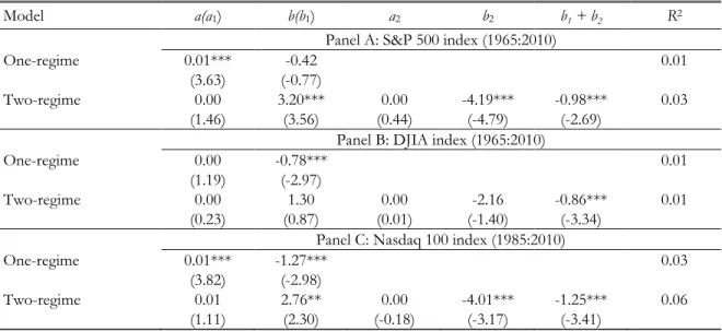
Table 6. S&P 500, DJIA and Nasdaq 100 excess returns against conditional variance in the rolling window model
The table reports the estimates and t-statistics of the rolling window model regressions in BW sentiment regimes: 𝑅𝑡+1 = 𝑎 + 𝑏𝑉𝑎𝑟𝑡(𝑅𝑡+1) + 𝜀𝑡+1, (3) 𝑅𝑡+1 = 𝑎1+ 𝑏1𝑉𝑎𝑟𝑡(𝑅𝑡+1) + 𝑎2𝐷𝑡+ 𝑏2𝐷𝑡𝑉𝑎𝑟𝑡(𝑅𝑡+1) + 𝜀𝑡+1, (4) 𝑉𝑎𝑟𝑡(𝑅𝑡+1) = 22 ∑ 𝑁1 𝑡 𝑁𝑡 𝑑=1 𝑟𝑡−𝑑2 , (1)
Rt + 1 is the monthly excess return on the NYSE-Amex index. Vart(Rt + 1) is the conditional variance. Dt is the
dummy variable for BW high-sentiment periods. rt-d is the daily demeaned NYSE-Amex index return (the daily
return minus the within-month mean). Nt is the number of trading days in month t, and 22 is the approximate
number of days in one month. Sample period is January 1965 to December 2010. The numbers in parentheses are t-statistics from the Newey-West standard error estimator. ***, **, * denote a 1%, 5% and 10% significance levels of the t-statistics, respectively.
Model a(a1) b(b1) a2 b2 b1 + b2 R2
Panel A: S&P 500 index (1965:2010)
One-regime 0.01*** -0.42 0.01
(3.63) (-0.77)
Two-regime 0.00 3.20*** 0.00 -4.19*** -0.98*** 0.03 (1.46) (3.56) (0.44) (-4.79) (-2.69)
Panel B: DJIA index (1965:2010)
One-regime 0.00 -0.78*** 0.01
(1.19) (-2.97)
Two-regime 0.00 1.30 0.00 -2.16 -0.86*** 0.01
(0.23) (0.87) (0.01) (-1.40) (-3.34)
Panel C: Nasdaq 100 index (1985:2010)
One-regime 0.01*** -1.27*** 0.03
(3.82) (-2.98)
Two-regime 0.01 2.76** 0.00 -4.01*** -1.25*** 0.06
(1.11) (2.30) (-0.18) (-3.17) (-3.41)
In the two-regime scenario, results vary considerably between models. Regarding the rolling window model, all the three stock indices allow sentiment to show the same ability to distinguish two clear patterns identical to what we observe in Section III. The mean-variance tradeoff is statistically significant – except for the DJIA index – and positive in the low sentiment periods (𝑏1 is 3.20 for the S&P 500 index, 1.30 for the DJIA index, and 2.76 for
24 Table 7. S&P 500, DJIA and Nasdaq 100 excess returns against conditional variance in GARCH (1,1)
The table reports the estimates and t-statistics of the GARCH (1,1) model regressions in BW sentiment regimes:
𝑅𝑡+1 = 𝑎 + 𝑏𝑉𝑎𝑟𝑡(𝑅𝑡+1) + 𝜀𝑡+1, (3)
𝑅𝑡+1 = 𝑎1+ 𝑏1𝑉𝑎𝑟𝑡(𝑅𝑡+1) + 𝑎2𝐷𝑡+ 𝑏2𝐷𝑡𝑉𝑎𝑟𝑡(𝑅𝑡+1) + 𝜀𝑡+1, (4)
𝑉𝑎𝑟𝑡(𝑅𝑡+1) = 𝜔 + 𝛼1𝜀𝑡2+ 𝛽𝑉𝑎𝑟𝑡−1(𝑅𝑡), (2)
Rt + 1 is the monthly excess return on the different stock indices. Vart(Rt + 1) is the conditional variance. Dt is
the dummy variable for BW high-sentiment periods. Sample period is January 1965 to December 2010. The numbers in parentheses are t-statistics from the Newey-West standard error estimator. ***, **, * denote a 1%, 5% and 10% significance levels of the t-statistics, respectively.
Model a(a1) b(b1) a2 b2 ω x 103 α β b1 + b2 Panel A: S&P 500 (1965:2010) One-regime 0.00 3.19 0.00** 0.11*** 0.85*** (0.15) (1.28) (2.11) (3.93) (25.29) Two-regime 0.00 4.77 0.00 -2.65 0.00** 0.11*** 0.85*** 2.13 (-0.06) (1.42) (0.09) (-0.52) (2.06) (3.89) (25.17) (0.27) Panel B: DJIA (1965:2010) One-regime 0.01 -4.63 0.00*** 0.04 -0.83*** (0.40) (-0.39) (12.77) (1.05) (-6.49) Two-regime -0.02 9.74 0.06 -33.53 0.00*** 0.05 -0.73*** -23.79 (-0.63) (0.64) (1.19) (-1.12) (8.76) (1.23) (-3.24) (-0.59) Panel C: Nasdaq 100 (1973:2010) One-regime 0.00 1.40 0.00* 0.12*** 0.81*** (0.49) (0.86) (1.73) (3.04) (11.35) Two-regime -0.01 5.20* 0.01 -5.19 0.00* 0.12*** 0.82*** 0.01 (-0.56) (1.66) (0.73) (-1.39) (1.77) (2.95) (12.57) (0.00)
the Nasdaq 100 index; t-statistics of 3.56, 0.87, and 2.30, respectively). During high-sentiment times, we observe a strong, statistically significant negative relation in all cases (𝑏1+ 𝑏2 is -0.98 with a t-statistic of -2.69, -0.86 with a t-statistic of -3.34, and -1.25 with a
t-statistic of -3.41 for S&P 500, DJIA and Nasdaq 100, respectively).
When looking at the GARCH (1,1) estimates, none of the indices allow sentiment to show the same ability to differentiate the two patterns. In fact, there is no consistent significant pattern, especially for the high-sentiment regime.
B. International evidence
Next, we explore the following empirical question: Is U.S. BW composite measure able to present the same ability to explain the mean-variance dynamics in other international
25 stock exchanges? And if so, does it suggest a leading role for U.S. sentiment in the global economy?
We explore data from Canada (SPTSX index), Germany (Dax index), France (CAC 40 index), U.K. (FTSE 100 index), and Japan (Nikkei 225 index) and try to answer the question. We use Bloomberg monthly time-series of raw returns (as proxies for each stock market returns) and the CRSP one-month T-bill returns (as our risk-free measure), in order to compute excess market returns from January 1965 to December 2010, which is also the BW (2006) sentiment index sample period. Yet, due to data availability constraints, we use different sample periods starting at 1970 for Japan excess returns, 1977 for Canada excess returns, 1984 for U.K. excess returns, and 1987 for France excess returns.
Table 8 accommodates the estimates and test-statistics from the regressions with the rolling window model as the conditional variance model for each country’s returns.The rolling window model shows that BW sentiment is equally effective at playing a decisive role in the mean-variance tradeoff of all countries but Japan, showing statistically significant ability to identify clear two-pattern regimes. Results suggest that when sentiment traders have a greater influence in the U.S. stock exchange, these countries see the risk-return dynamics of their stock markets change dramatically. During periods of high investor sentiment in the U.S. market, these countries’ mean-variance tradeoff is negative with statistical and economic significance. Canada and U.K., as it could be expected, seem to be the markets under greater influence of American sentiment traders. During low-sentiment periods, the mean-variance relation is positive and significant, whereas such relation presents to be greatly distorted when American sentiment traders play the market.
26 GARCH (1,1), in turn, suggests BW sentiment to be little if any effective in all countries, with results being not significant and inconclusive.8
Table 8. International excess returns against conditional variance in rolling window model
The table reports the estimates and t-statistics of the rolling window model regressions in BW sentiment regimes: 𝑅𝑡+1 = 𝑎 + 𝑏𝑉𝑎𝑟𝑡(𝑅𝑡+1) + 𝜀𝑡+1, (3) 𝑅𝑡+1 = 𝑎1+ 𝑏1𝑉𝑎𝑟𝑡(𝑅𝑡+1) + 𝑎2𝐷𝑡+ 𝑏2𝐷𝑡𝑉𝑎𝑟𝑡(𝑅𝑡+1) + 𝜀𝑡+1, (4) 𝑉𝑎𝑟𝑡(𝑅𝑡+1) = 22 ∑ 𝑁1 𝑡 𝑁𝑡 𝑑=1 𝑟𝑡−𝑑2 , (1)
Rt + 1 is the monthly excess return on each stock market index. Vart(Rt + 1) is the conditional variance. Dt is the
dummy variable for BW high-sentiment periods. rt-d is the daily demeaned NYSE-Amex index return (the daily
return minus the within-month mean). Nt is the number of trading days in month t, and 22 is the approximate
number of days in one month. Sample period is January 1965 to December 2010. The numbers in parentheses are t-statistics from the Newey-West standard error estimator. ***, **, * denote a 1%, 5% and 10% significance levels of the t-statistics, respectively.
Model a(a1) b(b1) a2 b2 b1 + b2 R2 Panel A: Germany (1965:2010) One-regime 0.00 -0.12 0.00 (0.25) (-0.20) (0.00) Two-regime 0.00 2.82* 0.00 -3.53** -0.72 0.01 (-0.99) (1.78) (0.77) (-2.04) (-1.21) Panel B: Canada (1977:2010) One-regime 0.00 -1.15** 0.01 (1.63) (-2.27) (0.00) Two-regime 0.00 3.10** 0.00 -4.42*** -1.32*** 0.03 (1.18) (2.43) (-0.62) (-3.61) (-2.77) Panel C: Japan (1970:2010) One-regime 0.00 -0.21 0.00 (-0.13) (-0.76) (0.00) Two-regime 0.00 -0.28 0.00 0.09 -0.19 0.00 (0.28) (-0.20) (-0.50) (0.06) (-0.96)
Panel D: United Kingdom (1984:2010)
One-regime 0.00 -0.63 0.00 (1.41) (-1.40) (0.00) Two-regime 0.00 3.78*** 0.00 -4.73*** -0.95** 0.03 (-0.30) (2.76) (0.47) (-3.23) (-2.34) Panel E: France (1987:2010) One-regime 0.00 -0.65 0.00 (0.68) (-1.13) (0.00) Two-regime 0.00 2.29* 0.00 -3.43** -1.15** 0.02 (-0.57) (1.71) (0.55) (-2.34) (-2.47)
8 We do not report the table with GARCH (1,1) estimates and test-statistics for this robustness check, but it can be made available upon request.
27 C. Comparing sentiment with macro-variables
It is widely discussed in sentiment literature the influence of business cycle variables upon any proxy of investor sentiment. One should bear in mind that both sentiment measures used in our work have been regressed on the growth in industrial production, the growth in durable, nondurable, and services consumption, the growth in employment, and on a flag for NBER recessions to control for macro-conditions, removing the effects of business cycle information. To compare the performance of a sentiment measure to the one of a macro-economic variable is thus a natural next step in our dissertation.
We consider five macro-variables commonly used in literature and run the empirical tests described in Section IV, and compare each variable’s ability to distinguish two-pattern regimes to the results we obtain with BW composite index. We use the one-year T-bill return as our interest rate; the term premium, defined as the return difference between the 30-year and one-month T-bills; the default premium computed as the return difference between AAA and BAA corporate bonds; and the dividend-price ratio, calculated as the ratio of the total dividend to the market value of all stocks on the NYSE-Amex index. From the website of the Federal Reserve at St. Louis we downloaded the AAA and BAA corporate bonds data and the consumption data. The remaining data is available at CRSP. We build on the methodology we use with investor sentiment and separate our sample into two regimes, above or below the median of each macro-variable. We run the same regressions structure [equations (1) and (2)] and define the dummy variable, 𝐷𝑡, is one for the low mean-variance
regime. We define low-sentiment periods as periods in which the macro-variable’s level is below its median. Tables 9 shows the estimates and test-statistics from the regressions with the rolling window model as the conditional variance model for each macro-economic variable.
28 The results are strongly conclusive and consistent across all macro-economic and for both variance models.9 Not a single one of the macro-variables could collect a set of equally
coherent and stable results, which fully corroborates YY (2011) findings. Overall, investor sentiment seems to possess a unique capacity to deliver the two-regime pattern in a cohesive and reliable way.
Table 9. Excess returns against conditional variance in rolling window model for macro-variables’ two-regime periods
The table reports the estimates and t-statistics of the rolling window model regressions in macro-variables’ two-regime periods: 𝑅𝑡+1 = 𝑎 + 𝑏𝑉𝑎𝑟𝑡(𝑅𝑡+1) + 𝜀𝑡+1, (3) 𝑅𝑡+1 = 𝑎1+ 𝑏1𝑉𝑎𝑟𝑡(𝑅𝑡+1) + 𝑎2𝐷𝑡+ 𝑏2𝐷𝑡𝑉𝑎𝑟𝑡(𝑅𝑡+1) + 𝜀𝑡+1, (4) 𝑉𝑎𝑟𝑡(𝑅𝑡+1) = 22 ∑ 𝑁1 𝑡 𝑁𝑡 𝑑=1 𝑟𝑡−𝑑2 , (1)
Rt + 1 is the monthly excess return on the NYSE-Amex index. Vart(Rt + 1) is the conditional variance. Dt is the
dummy variable for high-sentiment periods. rt-d is the daily demeaned NYSE-Amex index return (the daily
return minus the within-month mean). Nt is the number of trading days in month t, and 22 is the approximate
number of days in one month. Tbill is the return on the one-year T-bill; Def spread is the return difference between AAA and BAA corporate bonds; Term spread is the return difference between the 30-year and one-month T-bills; and D/P ratio is the ratio of the total dividend to the market value of all stocks on the NYSE-Amex index. Sample period is January 1965 to December 2010. The numbers in parentheses are t-statistics from the Newey-West standard error estimator. ***, **, * denote a 1%, 5% and 10% significance levels of the t-statistics, respectively.
Model a(a1) b(b1) a2 b2 b1 + b2 R2
Panel A: Equal-weighted returns
Tbill 0.00 -0.57 0.01* 0.18 -0.38 0.01 (1.08) (-0.82) (1.75) (0.14) (-0.34) Def spread 0.01*** -0.50 -0.01 -0.81 -1.30 0.01 (3.54) (-0.62) (-1.54) (-0.29) (-0.49) Term Spread 0.01*** -0.66 -0.01** 2.09 1.43 0.01 (4.78) (-0.84) (-2.32) (0.66) (0.47) D/P ratio 0.00 -0.14 0.01 -1.67 -1.80 0.01 (0.95) (-0.21) (1.54) (-0.50) (-0.98)
Panel B: Value-weighted returns
Tbill 0.00 -1.01*** 0.00 0.11 -0.90 0.01 (1.61) (-2.67) (0.79) (0.15) (-1.42) Def spread 0.01*** -1.15*** -0.01** 1.97 0.82 0.01 (3.57) (-3.05) (-2.20) (0.87) (0.37) Term Spread 0.01*** -1.16*** -0.01** 2.49 1.32 0.02 (4.41) (-3.10) (-2.52) (1.32) (0.71) D/P ratio 0.00 -0.70** 0.01* -1.28 -1.98 0.02 (0.74) (-2.32) (1.93) (-0.57) (-0.85)
9 We do not report the table with GARCH (1,1) estimates and test-statistics for this robustness check, but it can be made available upon request.
29 D. Trying an alternative GARCH model
Additionally, we use the asymmetric GARCH (1,1) as an alternative to the GARCH (1,1) to perform robustness tests. Glosten et al. (1993) build an asymmetric GARCH model to allow different impacts from positive and negative residuals. The asymmetric GARCH (1,1) models the conditional variance as:
𝑉𝑎𝑟𝑡(𝑅𝑡+1) = 𝜔 + 𝛼1𝜀𝑡2+ 𝛼2 𝐼𝑡 𝜀𝑡2+ 𝛽𝑉𝑎𝑟𝑡−1(𝑅𝑡), (5)
where 𝐼𝑡 is the dummy variable and takes the value one for positive shocks.
Table 10 accommodates the estimates and test-statistics from the regressions with the asymmetric GARCH (1,1) as the conditional variance model, and BW sentiment as the sentiment proxy.
Table 10. Excess returns against conditional variance in asymmetric GARCH (1,1)
The table reports the estimates and t-statistics of the asymmetric GARCH (1,1) model regressions in BW sentiment regimes:
𝑅𝑡+1 = 𝑎 + 𝑏𝑉𝑎𝑟𝑡(𝑅𝑡+1) + 𝜀𝑡+1, (3)
𝑅𝑡+1 = 𝑎1+ 𝑏1𝑉𝑎𝑟𝑡(𝑅𝑡+1) + 𝑎2𝐷𝑡+ 𝑏2𝐷𝑡𝑉𝑎𝑟𝑡(𝑅𝑡+1) + 𝜀𝑡+1, (4)
𝑉𝑎𝑟𝑡(𝑅𝑡+1) = 𝜔 + 𝛼1𝜀𝑡2+ 𝛼2𝐼𝑡𝜀𝑡2+ 𝛽𝑉𝑎𝑟𝑡−1(𝑅𝑡), (5)
Rt + 1 is the monthly excess return on the NYSE-Amex index. Vart(Rt + 1) is the conditional variance. Dt is the
dummy variable for BW high-sentiment periods. rt-d is the daily demeaned NYSE-Amex index return (the daily
return minus the within-month mean). Nt is the number of trading days in month t, and 22 is the approximate
number of days in one month. Sample period is January 1965 to December 2010. The numbers in parentheses are t-statistics from the Newey-West standard error estimator. ***, **, * denote a 1%, 5% and 10% significance levels of the t-statistics, respectively.
Model a(a1) b(b1) a2 b2 ω x 103 α1 α2 β b1 + b2
Panel A: Equal-weighted returns
One-regime -0.01 4.90* 0.17*** 0.10*** -0.01 0.85*** (-1.11) (1.68) (2.91) (3.93) (-0.44) (28.97)
Two-regime 0.00 5.34*** -0.01 -1.53 0.19*** 0.11*** -0.03 0.84*** 3.81 (-0.51) (2.96) (-0.94) (-0.63) (2.85) (3.60) (-0.86) (25.75) (0.99)
Panel B: Value-weighted returns
One-regime 0.00 2.76 0.06*** 0.09*** 0.09** 0.86*** (0.40) (1.34) (3.27) (3.52) (2.02) (34.43)
Two-regime 0.00 4.12*** 0.00 -0.32 0.08* 0.09*** 0.09* 0.85*** 3.80 (0.37) (5.36) (-0.53) (-0.08) (1.66) (3.47) (1.94) (24.61) (0.91)
Under the one-regime setting, the mean-variance relation, 𝑏, is positive and statistically significant for the asymmetric GARCH (1,1) model (𝑏 is 4.9 with a t-statistic of 1.68), which
30 opposes to the relation we find with the rolling window model but is consistent to the standard GARCH model result. Under the regime setting, again, we find the same two-pattern evidence we find in the GARCH (1,1): in low-sentiment periods, there is a strong and statistically significant positive tradeoff between the mean and the variance of returns expressed in the coefficient 𝑏1 (𝑏1 is 5.34 with a t-statistic of 2.96), whereas during
high-sentiment we find a positive but weak tradeoff (𝑏1+ 𝑏2 is -3.81 with a t-statistic of 0.99).
The literature has long reported conflicting conclusions dependent on the volatility methodology, and especially on the conditional variance models used. Particularly, Glosten et al. (1993) find these contradictory results between the standard GARCH and the asymmetric GARCH. Our results, however, are robust across both GARCH models used.
V. Conclusions
This work contributes to the existing sentiment literature by presenting unequivocal evidence of the critical role investor sentiment plays on the mean-variance relation. We show that during high-sentiment periods investor sentiment undermines an otherwise positive mean-variance tradeoff. In low-sentiment periods, the common understanding holds that investors should obtain a compensation for bearing variance risk. Our results are aligned with the argument that there is a larger intervention and greater influence of sentiment traders in the markets when sentiment is high. We additionally add to the scarce international evidence existent in the sentiment literature, describing the same mean-variance tradeoff for five other countries, in which we suggest U.S. sentiment may have a leading role in the other countries’ stock markets and directly impact their dynamics.
Our approach represents by construction a different mechanism for sentiment to commove with stock prices, when compared to the widely understood practices. Most
31 empirical works study its direct effects on prices, in which prices commove with investor sentiment. We show that sentiment rather affects the compensation for bearing variance risk first, and as result, price levels.
This works contributes simultaneously to the extensive mean-variance literature. Although this has been such a thoroughly researched topic, there is no consensus on the nature of the tradeoff. By documenting that investor sentiment distorts the tradeoff in periods of high sentiment, we bring awareness to the need for models of stock prices that accurately accommodate investor sentiment and emphasize its significant part on the risk-return affair.