Arrestment of the estuarine plume in Maputo bay, Mozambique

(1)

Katrin Markull

Arrestment of the Estuarine Plume in Maputo Bay,

Mozambique

Aprisionamento da Pluma Estuarina na Baía de

Maputo, Moçambique

(2)

(3)

Katrin Markull

Arrestment of the Estuarine plume in Maputo Bay,

Mozambique

Aprisionamento da Pluma Estuarina na Baía de

Maputo, Moçambique

Dissertação apresentada à Universidade de Aveiro para cumprimento dos requisitos necessários à obtenção do grau de Mestre em Ciências do Mar e das Zonas Costeiras, realizada sob a orientação científica do Prof. Doutor João Miguel Sequeira Silva Dias, Professor Auxiliar do Departamento de Física da Universidade de Aveiro e co-orientação do Doutor João Daniel Alonso Antão Lencart e Silva, Investigador Auxiliar no Centro de Estudos do Ambiente e do

(4)

(5)

o júri

Presidente Prof.ª Doutora Filomena Maria Cardoso Pedrosa Ferreira Martins

Professora Associada do Departamento de Ambiente e Ordenamento da Universidade de Aveiro

Arguente Doutor Nuno Alexandre Firmino Vaz

Investigador auxiliar do CESAM e Departamento de Física da Universidade de Aveiro

Orientador Prof. Doutor João Miguel Sequeira Silva Dias

(6)

(7)

acknowledgements This study was only possible thanks to the help, support and active collaboration of many people.

To Prof. Doutor João Miguel Dias for suggesting this interesting topic for my MSc thesis, for the scientific supervision and for always having been available for any doubts and questions I had.

To Doutor João Daniel Alonso Antão Lencart e Silva, for everything he taught me over the past months, never losing patience and a positive attitude, as well as for having allowed me to use his scientific data of Maputo Bay.

To the NMEC working group, for their availability, support and encouragement, especially during the last months.

To my great friends, for their presence even though some only from the distance.

To Sarah and Guilherme, for their friendship, understanding and support. To my family, whose support I could always count on.

To Miguel for the unconditional support and understanding in these last months.

(8)

(9)

keywords Estuarine dynamics; hydrodynamic modeling; Delft3D; salinity; flushing times; tide; stratification; river flow

abstract Maputo Bay is a tidally-energetic embayment in Mozambique, influenced by strong rainfall and associated river runoff during the wet season. Previous investigations have suggested the arrestment of the freshwater plume related to high mixing during spring tide, eroding stratification and preventing an efficient exchange with the shelf due to the hampering of density currents. It was suggested that, with decreasing mixing towards neap tide, the bay would re-stratify, releasing the estuarine plume. The objective of this dissertation was to find out whether and under which conditions this arrestment of the estuarine plume occurs in Maputo Bay.

A 3-dimensional hydrodynamic model was applied to the bay, improving a previously published model through vertical and temporal refinement and recalibration. It is shown that now the model reproduces more accurately the semidiurnal and fortnightly stratification-mixing cycles occurring during the wet season. However, the model still predicts salinities lower than those found in observations. Uncertainties increase towards the mouth of the Maputo River, for which only modelled river flow data was available to force the bay dynamics, indicating this input as a possible source of the underestimation of salinity. The effect of varying river discharges, varying timings of discharge as well as varying discharge ratios on flushing times was investigated through a set of experiments of varying Maputo and Incomati river flows as well as timings of discharge during the spring-neap cycle.

The results suggest that when no discharge or a small discharge is introduced, flushing times are smallest during spring tide, when barotropic forcing is strong. Largest flushing times are found approximately 40 hours before neap tide, when tidal forcing is relatively weak. Flushing times for model runs with larger discharge were smaller due to the addition of flushing from river water. Here, flushing times were especially small during neap tide, when the decreased tidal mixing lead to stratification through which a classical estuarine circulation could develop, leading to an efficient bay-shelf exchange. Maximum flushing times for high-discharge runs during wet season were found for spring tide. Shelf-bay exchange was most efficient when the discharge of the Maputo River was larger than the discharge of the Incomati River, due to its location opposite the bay opening, thus influencing a larger area before leaving the bay. Timing of the discharge of the freshwater had only small effects, influencing the amount of mixing induced on the freshwater when first entering the bay.

It is concluded that the estuarine plume of Maputo Bay is in fact arrested during spring tide due to the large mixing inhibiting density currents and is released when mixing decreases, inducing stratification and baroclinic circulation. The potential energy stored in the bay is larger for a larger discharge of the Maputo River.

(10)

(11)

palavras-chave Dinâmica estuarina; Delft3D, modelação hidrodinâmica; salinidade; tempos de renovação, maré; estratificação; escoamento fluvial

resumo A Baía de Maputo, em Moçambique, é uma baía com marés energéticas, influenciada pelo escoamento dos rios associado a forte precipitação durante a estação húmida. Investigações anteriores têm sugerido que o aprisionamento da pluma de água doce está relacionado com a elevada mistura durante a maré viva, que por sua vez provoca a erosão da estratificação e impede a troca eficiente com a plataforma continental, dificultando o estabelecimento de correntes de densidade. Foi sugerido que com a diminuição da mistura durante a maré morta a baía seria re-estratificada, libertando a pluma estuarina. O objetivo desta dissertação foi averiguar se, e em que condições, este aprisionamento da pluma estuarina ocorre na baía de Maputo.

Foi aplicado um modelo hidrodinâmico 3-d para a baía, resultante do melhoramento de um modelo publicado anteriormente, através do refinamento vertical e temporal e recalibração. É demonstrado que agora o modelo reproduz com mais precisão os ciclos de estratificação/mistura semidiurnas e quinzenais que ocorrem durante a estação chuvosa. No entanto, o modelo ainda prevê salinidades inferiores as encontradas em observações. As incertezas aumentam próximo da foz do Rio Maputo, para o qual existem apenas dados de modelos de bacia para forçar o modelo, indicando esta entrada como uma possível causa da subestimação da salinidade. Foi definido um conjunto de experiências de diferentes descargas dos Rios Maputo e Incomati, sendo estes introduzidos no modelo em fárias fases do ciclo da maré. Foi investigado o efeito da variação da duração das descargas fluviais e da proporção do Maputo e do Incomati nos tempos de renovação da água na baía.

Os resultados sugerem que quando há uma pequena descarga dos rios, os tempos de renovação são menores durante a maré viva, quando o forçamento barotrópico é forte. Os maiores tempos de renovação encontram-se cerca de 40 horas antes da maré morta. Os tempos de renovação para as corridas com maior descarga são menores devido à adição de descargas de água do rio. Neste caso, os tempos de renovação foram especialmente pequenos durante a maré morta, quando a diminuição da mistura pela maré induz estratificação, criando condições para o desenvolvimento da circulação estuarina clássica, e escoando a baía eficiente. Tempos máximos de renovação para corridas de alta descarga durante a estação chuvosa foram encontrados em condições mistas de maré viva. O intercâmbio entre a baía e a plataforma continental foi mais eficiente para uma maior proporção do Rio Maputo em relação ao Rio Incomati. Este padrão justifica-se pela maior distância da foz do Rio Maputo à entrada da baía. A variação do momento da descarga de água doce em relação à fase da maré tem efeitos pouco significativos (ou pouco relevantes), determinando apenas o grau de mistura que influencia a água doce nas primeiras horas a seguir da descarga.

Concluiu-se que existe um aprisionamento da pluma estuarina da Baía de Maputo. Este aprisionamento ocorre durante a elevada mistura de maré viva. A energia potencial armazenada na baía é maior para uma descarga maior do Rio Maputo.

(12)

(13)

1

List of Figures

FIGURE 1: LOCATION AND BATHYMETRIES OF MAPUTO BAY ... 8

FIGURE 2: REGIONAL OCEANOGRAPHIC CONTEXT OF MAPUTO BAY ... 15

FIGURE 3: COMPARISON OF THE SIGMA-GRID (LEFT) AND THE Z-GRID (RIGHT) (DELTARES, 2011), ... 16

FIGURE 4: BATHYMETRY AND GRID OF MAPUTO BAY ... 26

FIGURE 5: COMPARISON BETWEEN OBSERVATIONS AND MODEL RESULTS OF SSE TIME SERIES ... 27

FIGURE 6: COMPARISON BETWEEN OBSERVATIONS AND MODEL PREDICTIONS OF TIDAL CURRENTS ... 29

FIGURE 7: COMPARISON BETWEEN PREDICTED AND OBSERVED TIDAL AMPLITUDES FOR SEVERAL CONSTITUENTS ... 30

FIGURE 8: COMPARISON BETWEEN PREDICTED AND OBSERVED PHASES FOR SEVERAL CONSTITUENTS ... 31

FIGURE 9: COMPARISON OF PREDICTED AND OBSERVED SEASONAL EVOLUTION OF BAY-AVERAGE SALINITY AND WATER TEMPERATURE WITH FORCING AGENT RIVER FLOW ... 32

FIGURE 10: OBSERVED WATER COLUMN PROPERTIES AT SECTION CB DURING SPRING TIDE ... 34

FIGURE 11: PREDICTED WATER COLUMN PROPERTIES AT SECTION CB DURING SPRING TIDE FOR THE NEW MODEL ... 35

FIGURE 12: PREDICTED WATER COLUMN PROPERTIES AT SECTION CB DURING SPRING TIDE FOR THE OLD MODEL ... 36

FIGURE 13: OBSERVED WATER COLUMN PROPERTIES AT SECTION CB DURING NEAP TIDE ... 37

FIGURE 14: PREDICTED WATER COLUMN PROPERTIES AT SECTION CB DURING NEAP TIDE FOR THE NEW MODEL ... 38

FIGURE 15: PREDICTED WATER COLUMN PROPERTIES AT SECTION CB DURING NEAP TIDE FOR THE OLD MODEL ... 39

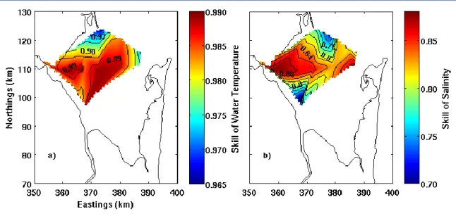
FIGURE 16: SKILL VALUES FOR A) WATER TEMPERATURE AND B) SALINITY, INTERPOLATED OVER PART OF THE BAY ... 41

FIGURE 17: MAPS OF BAY-WIDE SALINITY RMSE DISTRIBUTION OVER TIME ... 42

FIGURE 18: COMPARISON OF RMSE OF SALINITY PER STATION ... 43

FIGURE 19: PATTERN OF VARYING DURATIONS OF DISCHARGE PULSES FOR WET SEASON RUNS. ... 48

FIGURE 20: GRID AREA INCLUDED IN THE MASK TO CALCULATE BAY-AVERAGE VALUES ... 50

FIGURE 21: BATHYMETRY OVER THE BAY'S OPENING. ... 53

FIGURE 22: VARIATION OF SALINITY DIFFERENCES BETWEEN BOTTOM AND SURFACE LAYER ACROSS MAPUTO BAY'S MOUTH FOR EXTREME DISCHARGE DURING THE DRY SEASON AT A) SPRING TIDE ... 55

FIGURE 23: TIDALLY-FILTERED BAY-AVERAGE SALINITIES OVER TIME DURING DRY SEASON ... 58

FIGURE 24: VARIATION OF WATER TEMPERATURE DIFFERENCES BETWEEN BOTTOM AND SURFACE LAYER ACROSS MAPUTO BAY'S MOUTH FOR RUNS WITHOUT RIVER DISCHARGE DURING DRY SEASON ... 60

FIGURE 25: VARIATION OF WATER TEMPERATURE DIFFERENCES BETWEEN BOTTOM AND SURFACE LAYER ACROSS MAPUTO BAY'S MOUTH FOR EXTREME RIVER DISCHARGE DURING DRY SEASON ... 61

FIGURE 26: DEVELOPMENT OF Φ OVER TIME ALONG MAPUTO BAY'S MOUTH, FOR MODEL START DURING SPRING TIDE IN DRY SEASON ... 63

FIGURE 27: DEVELOPMENT OF Φ OVER TIME ALONG MAPUTO BAY'S MOUTH, FOR MODEL START BETWEEN SPRING AND NEAP TIDE IN DRY SEASON ... 64

FIGURE 28: DEVELOPMENT OF Φ OVER TIME ALONG MAPUTO BAY'S MOUTH, FOR MODEL START DURING NEAP TIDE IN DRY SEASON ... 65

FIGURE 29: DEVELOPMENT OF Φ OVER TIME ALONG MAPUTO BAY'S MOUTH, FOR MODEL START BETWEEN NEAP AND SPRING TIDE IN DRY SEASON ... 66

FIGURE 30: DEVELOPMENT OF Φ OVER TIME ALONG MAPUTO BAY'S MOUTH, FOR MODEL START DURING SPRING TIDE AND EXTREME RIVER DISCHARGE WITH VARYING INCOMATI : MAPUTO RIVER DISCHARGE RATIOS DURING DRY SEASON ... 69

FIGURE 31: DEVELOPMENT OF Φ OVER TIME ALONG MAPUTO BAY'S MOUTH, FOR MODEL START DURING NEAP TIDE AND EXTREME RIVER DISCHARGE WITH VARYING INCOMATI : MAPUTO RIVER DISCHARGE RATIOS DURING DRY SEASON ... 70

FIGURE 32: RESIDUAL VELOCITIES FOR DRY SEASON MODEL RUNS STARTING AT SPRING TIDE ... 73

FIGURE 33: RESIDUAL VELOCITIES FOR DRY SEASON MODEL RUNS STARTING BETWEEN SPRING AND NEAP TIDE ... 74

FIGURE 34: RESIDUAL VELOCITIES FOR DRY SEASON MODEL RUNS STARTING AT NEAP TIDE ... 75

(16)

FIGURE 38: DEVELOPMENT OF DRY SEASON FLUSHING TIME FOR 5-DAY MOVING WINDOWS ... 82

FIGURE 39: DEVELOPMENT OF DRY SEASON RESIDENCE TIME FOR 5-DAY MOVING WINDOWS FOR VARYING DISCHARGE RATIOS .. 84

FIGURE 40: TIDALLY-FILTERED BAY-AVERAGE SALINITIES OVER TIME FOR WET SEASON RUNS WITH VARYING DISCHARGE RATIOS . 87 FIGURE 41: WET SEASON DEVELOPMENT OF Φ OVER TIME ALONG MAPUTO BAY'S MOUTH, FOR MODEL START DURING SPRING TIDE AND VARYING INCOMATI : MAPUTO RIVER DISCHARGE RATIOS ... 89

FIGURE 42: WET SEASON DEVELOPMENT OF Φ OVER TIME ALONG MAPUTO BAY'S MOUTH, FOR MODEL START DURING NEAP TIDE AND VARYING INCOMATI : MAPUTO RIVER DISCHARGE RATIOS ... 90

FIGURE 43: WET SEASON RESIDUAL VELOCITIES FOR MODEL RUNS WITH VARYING DISCHARGE RATIOS, STARTING AT SPRING TIDE 92 FIGURE 44: WET SEASON RESIDUAL VELOCITIES FOR MODEL RUNS WITH VARYING DISCHARGE RATIOS, STARTING AT NEAP TIDE .. 93

FIGURE 45: DEVELOPMENT OF FLUSHING TIMES FOR WET SEASON RUNS WITH VARYING DISCHARGE RATIOS ... 94

FIGURE 46: BAY-AVERAGE SALINITIES FOR WET SEASON RUNS WITH VARYING DISCHARGE DURATIONS AND TIMINGS ... 98

FIGURE 47: WET SEASON DEVELOPMENT OF Φ OVER TIME ALONG MAPUTO BAY'S MOUTH, FOR MODEL START DURING SPRING TIDE AND VARYING DURATIONS OF DISCHARGE ... 100

FIGURE 48: WET SEASON DEVELOPMENT OF Φ OVER TIME ALONG MAPUTO BAY'S MOUTH, FOR MODEL START DURING NEAP TIDE AND VARYING DURATIONS OF DISCHARGE... 101

List of Tables

TABLE 1: MONTHLY AVERAGE MAXIMUM AND MINIMUM AIR TEMPERATURES IN MAPUTO (CLIMATEMPS, 2013)... 10

TABLE 2: PERCENTAGE OF DEPTH PER LAYER ... 26

TABLE 3: ERROR VALUES FOR TIDAL WATER LEVELS AND CURRENTS ... 28

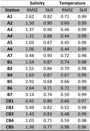
TABLE 4: RMSE AND SKILL VALUES FOR SALINITIES AND WATER TEMPERATURES PER SECTION... 40

TABLE 5: RMSE AND SKILL VALUES FOR SALINITIES AND WATER TEMPERATURES PER STATION ... 40

TABLE 6: RMSE AND SKILL VALUES FOR SALINITIES AND WATER TEMPERATURES PER SURVEY ... 41

TABLE 7: MODELLING SPECIFICATIONS FOR MAPUTO BAY ... 45

(17)

1

1 Introduction

This dissertation investigates the hydrodynamics of Maputo Bay, Mozambique, under varying forcing conditions. The first chapter provides a general introduction to the topic.

Firstly, in section 1.1, a general introduction will be given and the motivation and aim of this dissertation are presented. Section 1.2 will introduce the state of the art of the arrestment of estuarine plumes, induced by local or distant wind as well as by tidal forcing. Section 1.3 will then present the work structure for the complete dissertation.

1.1 Background, Motivation and Aim

Estuaries are diverse and complex dynamic regions in the transitional zone between land and sea. Due to their rich ecosystems and natural navigational facilities, they often support human concentration and the associated economic activities such as fisheries, transport and tourism. These activities can pose threats on the ecosystems that need to be studied to be fully understood and addressed.

The importance of the several forcing mechanisms involved in estuarine dynamics varies from estuary to estuary. Density-driven circulation in estuaries is usually influenced by river inflow. Other possible factors of importance include tidal dynamics and wind-induced circulation on the continental shelf as well as locally. The competition between the various forcing mechanisms as well as other factors such as topography and Coriolis force determine the so-called buoyancy-stirring interaction described by Simpson (1997). Different salinity distributions and circulation patterns are found, depending on the relative importance of buoyancy/stratification and stirring. River flow induces buoyancy in estuaries. The freshwater input leads to the development of horizontal gradients, with lighter water moving down-estuary in the upper layers and more dense water moving upstream in the deeper layers. This is known as classical estuarine circulation and induces stratification. Mixing can occur on the interface between fresher river water and more saline sea water (Simpson et al., 1990; Dyer, 1998).

Tides in the ocean are generated by centrifugal and gravitational forces of sun and moon. They influence estuaries mainly through barotropic processes arising from an oscillating pressure gradient (Simpson and Sharples, 1991; Officer, 1976). These pressure gradients then drive a circulation into and out of the estuary mouth, leading to tidal currents in the estuary. Most of the tidal energy that reaches the continental shelf is not reflected back into the deep ocean but dissipated in the shelf waters due to friction created in the bottom boundary layer and penetrating up the water column (Simpson, 1998). Through the friction, energy from the flow is transformed into turbulent eddies, inducing stirring. A large proportion of the turbulent kinetic energy is transferred into several decreasing scales of turbulent energy, down to molecular turbulence. If, however, the water column is stratified, some of the turbulent kinetic energy is also used to induce vertical mixing (Simpson, 1998). Apart from inducing stirring, tides can also lead to periodic stratification where horizontal density gradients exist. The vertical shear inserted by tides acts on the existing horizontal density gradients (Simpson et al., 1990). This can, if

(18)

horizontal density gradients are sufficiently strong, lead to distortions of the previously vertical isohalines due to surface layers being able to move faster than bottom layers, thus inducing stratification during ebb. In the flood the tide forces heavier water on top of lighter water. This leads to instability and buoyancy production of TKE (Turbulent Kinetic Energy) and then to vertical mixing contributing again to vertical isopycnals and to horizontal gradients, thus introducing periodic fluctuations. This process is called Strain-Induced Periodic Stratification (SIPS). Varying bathymetries can furthermore lead to the so-called tidal rectification, in which residual currents are developed due to the tidal waves travelling over varying topography, often creating a net outflow in deeper channels and a net inflow in more shallow areas (Li and O’Donnell, 1997). Wind can affect estuarine dynamics in a number of ways: remote wind can have effects on the density field and, through a rise or fall of the sea-level at the bay mouth, force the sea level and currents in the estuary. Furthermore local wind over the estuary can directly lead to surface currents. Through the shear stress that the moving air exerts on the water surface, friction can lead to mixing. Waves from distant and local wind can further lead to increased mixing of the water column. Wind forcing depends both on magnitude and direction of the wind and can also induce significant wave stirring induced by non-local winds (Simpson, 1997).

Atmospheric forcing can influence the stratification of the water column of estuaries by warming or cooling the surface layer or inducing buoyancy at the water surface through rain (Simpson et al., 1990).

Flushing times in estuaries vary largely and depend on various factors, including freshwater discharge and tidal forcing.

Several authors including Piedracoba et al. (2005), Chao (1988) and Lencart e Silva (2007) have suggested that estuarine plumes can be arrested under certain conditions, leading to increased flushing times in the estuary. Two mechanisms that can lead to this arrestment are:

 downwelling winds leading to the partial blocking off of the estuary mouth;

 the buoyancy-stirring interaction induced by large tidal variations leading to turbulence modulations, as explained theoretically by Linden and Simpson (1988).

Linden and Simpson (1986) and Linden and Simpson (1988) undertook laboratory experiments on the influence of turbulence on mixing and frontogenesis and compared their results to three case studies. Through air bubbles, turbulence was induced to a fluid containing a horizontal density gradient. Those authors suggested that, during periods of large turbulence e.g. through tidal mixing, the water column was vertically mixed and baroclinic circulation was weak. When turbulence was decreased, the baroclinic circulation accelerated while the water column stratified. A vertical density gradient developed through the denser fluid having been advected underneath the lighter fluid. The flow furthermore transported mass horizontally. Depending on the duration of the absence of turbulence, a front developed, in which the horizontal density gradient was increased. Once turbulence was increased again, the water column mixed vertically, reducing baroclinic circulation. Density was therefore transported horizontally through turbulence in the phases where air bubbling was increased and through baroclinic circulation in the absence of bubbles, with the latter being more effective. Linden and Simpson (1988) therefore concluded

(19)

3 that the exchange through a cross-gradient section is greater when the baroclinic circulation has

more time to develop, i.e. periods between turbulence are larger.

This study will concentrate on the second possible mechanism triggering the arrestment of estuarine plumes. The study area is Maputo Bay in Mozambique.

Maputo Bay is a shallow, subtropical estuary with a surface area of 1875 km². It is tidally-energetic with a large spring:neap tide ratio and characterised by highly varying river run-off. Its coastal resources are economically important for the area. Ravikumar et al. (2004) have shown that salinity can regulate the nutrient cycle in mangrove estuarine ecosystems. Salinities outside the 20 – 30 range will hamper production in the mangroves and affect the early life stages in mangrove habitats that sustain the economically important shrimp stocks (Monteiro and Marchand, 2009). The salinity of Maputo Bay is, for a part, controlled by dam systems of its main rivers. The density-driven circulation is strongly influenced by the neap-spring cycle. Here, a candidate mechanism for the arrestment of the plume is found in the wet season during spring tide, associated with turbulent mixing. During neap tide, the plume can then spread offshore. Lencart e Silva (2007) has suggested the occurrence of this arrestment of estuarine plumes induced by the large freshwater discharge in the wet season, in combination with decreased density forcing during high mixing periods associated with spring tide. This arrestment can influence salinities in the bay, decreasing salinities during times of arrestment.

The above-mentioned phenomenon in Maputo Bay has in the past been suggested from observations. In this study, modelling will be applied to research the conditions under which the arrestment as well as the release of the estuarine plume occurs. The three-dimensional model Delft3D-flow will be applied, using a set of scenarios and investigating flushing times under varying river discharge and tidal conditions. The dissertation will be concerned with the determination of conditions of the storage and release of the estuarine plume in Maputo Bay. A passive tracer will be introduced into the model to determine flushing times. A cross-section across the estuary opening will help determine stratification, velocities and salinity structures at this interface between the estuary and the shelf region.

The influence of varying discharge ratios of the two main rivers Incomati and Maputo will be investigated to find out the relative importance of the two rivers in setting the salinity and density field as well as influencing flushing times.

A set of scenarios of varying total discharge, discharge ratios between the rivers Incomati and Maputo as well as the timing of the discharge in wet and dry season conditions as well as within the spring-neap cycle is developed. A number of runs are conducted with varying durations of discharge to investigate whether managing the duration of the discharge can help maintaining salinities within the 20-30 range, providing optimal conditions for the bay’s ecosystem.

The aim of this dissertation is to investigate:

 Possible conditions of the arrestment and release of the estuarine plume;

 The influence of different amounts of discharge of the Incomati and Maputo Rivers into Maputo Bay;

(20)

 The influence of the timing of the discharge in the spring-neap tidal cycle on the bay dynamics and flushing times;

 The relative influence of the rivers Incomati and Maputo on the bay dynamics and flushing times;

 The influence of varying discharge durations on bay-average salinities.

Getting a better insight into the flushing times in estuaries is crucial to understanding the estuarine dynamics. Firstly, maintaining a maximum salinity can be important for the sustainability of economically important resources. Secondly, the dilution and transportation of pollutants in the estuary also depend on the flushing times and can strongly be influenced by an arrestment of the estuarine plume.

The following sub-chapter will focus on the state of the art on the arrestment of estuarine plumes. For an introduction and state of the art on the study area Maputo Bay, please refer to Chapter 2.

1.2 The Arrestment of Estuarine Plumes: State of the Art

Literature suggests that local onshore winds as well as remote winds on the continental shelf may lead to a decrease of flushing of estuaries. Furthermore can the buoyancy-stirring interaction induced by large tidal variations lead to turbulence modulations which in turn can arrest the estuarine plume during high mixing of spring tide. This chapter will give a review on some of these investigations. Firstly, an overview of previous investigations concerning wind-induced forcing will be given. Next, an introduction on tide-induced arrestment is given.

Wind-induced

Local wind-induced forcing

Geyer (1997) investigated the effect of local on- and offshore winds on the flushing times of two shallow estuaries in Cape Cod, U.S.A., through observations. That author found that in both, the Childs River estuary and the Quashnet River estuary, onshore winds reduce estuarine circulation and along-estuary salinity gradients increase due to the accumulating freshwater. Through the inhibited estuarine circulation, flushing rates are reduced. Offshore winds, on the other hand, flush out estuarine water, reduce along-channel salinity gradients and lead to increased flushing. That author furthermore found that a constriction, in this case bridge abutments, restrict the flushing of both estuaries.

DeCastro et al. (2003) used a combination of observations and the hydrodynamic model MOHID to examine the influence of local winds on the exchange between the shelf and the Ria de Ferrol, one of the Galician Rias Baixas. They found that the wind-induced flow through the 350 m-wide Strait of Ferrol under real wind conditions can be around 1.5 % of the total flow (20 m3s-1 due to wind, 1200 m3s-1 due to tidal forcing and 2.5 m3s-1 due to freshwater input in summer) and is therefore the main cause of residual circulation. Wind forcing leads to an asymmetric ebb-flood

(21)

5 cycle, with surface currents being offset by 0.5 ms-1, with the offset decreasing with depth and

eventually changing sign in deeper layers.

DeCastro et al. (2000) investigated the influence of tides and local winds on the circulation in the Galician Ria de Pontevedra through observations. They found that wind speeds higher than 4 ms-1 can dominate the surface currents, leading to a reversal of the normal tidal circulation. During moderate offshore winds with average wind speeds of 5-7 ms-1, surface currents were controlled by winds, leaving the Ria even against tidal forcing, while bottom layer currents were tidally controlled. Moderate onshore winds with wind speeds of 7-12 ms-1 forced shelf water to enter the estuary through surface layers, while bottom layers behaved according to the tidal regime, leaving the estuary.

Chao (1988) examined the behaviour of estuarine plumes during different wind events through the application of a three-dimensional primitive-equation model. That author found that a local onshore wind can inhibit gravitational circulation in an estuary, destroy the plume structure on the shelf and accumulate fresh water in the estuary. Once the wind relaxes, a new plume quickly develops, transporting the lower-salinity water out of the estuary, onto the shelf. If the onshore wind is relatively weak compared to buoyancy forcing, a three-layer circulation pattern can also develop, with a landward surface current of shelf water directed into the estuary, below which the positive estuarine circulation is found.

Distant wind-induced forcing

Various investigations over the last years have shown the possibility of the arrestment of estuarine circulation induced by remote winds, often related to downwelling-events blocking the outflow of estuarine surface waters.

Álvarez-Salgado et al. (2000) investigated the influence of upwelling and downwelling winds on the Galician Rias Baixas through observations and a two-dimensional box model. These authors found that during downwelling events, surface shelf waters piled up along the coast and entered the ria, preventing ria waters from leaving the estuary.

Prego et al. (1990) found southerly winds blocking the interchange between the shelf and the Ria de Vigo, leading to a half-closed estuarine circulation due to downwelling.

Piedracoba et al. (2005) investigated the influence of remote and local winds on the residual circulation and thermohaline variations in the Ria de Vigo through observations in 2002. Those authors found that southerly winds lead to a reversed circulation pattern in which the fresh water from river discharge was piled up in surface layers while an outgoing current was established in the bottom layers, transporting higher salinity waters out of the estuary. These findings were also confirmed by Gilcoto et al. (2007).

Chao (1988) applied a three-dimensional primitive-equation model to study the effect of local and shelf winds on estuarine plumes. That author found a hindering of the buoyancy-driven outflowing surface current due to the Ekman drift being directed onshore, leading to surface

(22)

currents being weakly downwind. Freshwater export from the estuary onto the shelf was retarded and lead to an increased content of fresh water in the estuary.

Dale et al. (2004) applied a two-dimensional box model to the Ria de Pontevedra, Galicia, to research water exchange with the shelf and flushing times in the estuary. They found that with the presence of a downwelling front in September and October 1998, freshwater was retained in the estuary, with gravitational circulation having been suppressed and flushing times increased in both the inner and central parts of the estuary.

Valle-Levinson et al. (1998) observed the passage of two downwelling wind periods near Chesapeake Bay with similar magnitudes and durations which produced very different hydrodynamic conditions in the bay. One wind event occurred during neap tide and lead to significant stratification after the wind had ceased. The other wind event occurred during spring tide and had produced much weaker stratification. In the wind event that occurred during neap tide, stirring through tides was less strong, therefore stratification developed in the estuary, increasing flushing. After the event that occurred during spring tide, on the other hand, tidal mixing was much stronger, decreasing vertical salinity gradients and retarding the flushing of the accumulated freshwater. Those authors therefore suggest that stronger mixing such as through tides can retard flushing.

Tide-induced

Another possible mechanism for the arrestment of estuarine circulation is related to tidal forcing, where a large spring: neap ratio exists.

The tides influence the flushing of an estuary through four mechanisms:  Tidal shear dispersion;

 Chaotic dispersion;  Tidal rectification;

 Tidal advection into shelf currents.

Chaotic dispersion occurs when an oscillatory field is superimposed on a constant field, resulting in a chaotic field. This may occur as a combination of tidal rectification and tidal velocity as described by Ridderinkhof and Zimmermann (1992).

The laboratory experiments by Linden and Simpson (1986) and Linden and Simpson (1988) that were explained in the introduction have shown the correlation between turbulence, stratification and mixing. Linden and Simpson (1988) furthermore compared their laboratory experiments with field observations in three regions where turbulence is induced through tidal stirring.

One of these is Spencer Gulf, a shallow bay in Southern Australia, characterised by hypersaline conditions, making Spencer Gulf a negative estuary. Nunes and Lennon (1987) found that during periods of low turbulence due to light winds in combination with the absence of semidiurnal currents, stratification developed. This occurred on a 14-day cycle due to the equality in amplitude of the lunar and solar semidiurnal tidal constituents. Those authors observed the

(23)

7 development of stratification arising from horizontal density advection when turbulence was very

weak. A buoyancy driven circulation developed and adjusted geostrophically to form a large cyclonic gyre. A boundary current into the gulf transported lower salinity water along the western coast while a counterflow transported the saline gulf water along the eastern coast out of the gulf, in accordance with the effect of the Earth’s rotation. Salinity differences between in- and outflow of >1 were possible and the gyre therefore lead to the flushing of excess salt from the gulf and the renewal of its water. The onset of winds or tidal currents was able to erode this gyre by mixing the water column again.

Another case study discussed by Linden and Simpson (1988) is that by Simpson et al. (1988), who investigated the control of tidal straining, density currents and stirring on estuarine stratification. Observations in Liverpool Bay showed an alternation between stratified and vertically mixed conditions with semidiurnal frequencies. Maximum stratification occurred during low water slack and Simpson et al. (1988) assumed that this alternation was due to tidal straining. Those authors furthermore found lower frequency periods of more permanent stratification coinciding with weak mixing during neap tides, probably due to reduced tidal mixing allowing an increase in the density current. In Liverpool Bay, those authors therefore concluded from observations and simulations that the semidiurnal signal of stratification pulses was intensified during spring tide and weakened during neap tides, when tidal mixing was weaker. They furthermore argued that in stronger tidal stream amplitudes tidal stirring will become more relevant in comparison with straining, with complete mixing occurring over most of the semidiurnal cycle, with strain induced stratification occurring near neap tide only.

Lencart e Silva (2007) observed the onset and breakdown of stratification during the wet season in Maputo Bay. During neap tides, when tidal stirring was at its minimum, a vertical density gradient established and baroclinic currents were found. A 3-dimensional hydrodynamic model was applied and results suggested that during high mixing of spring tides the estuarine plume was arrested, decreasing overall salinities of Maputo Bay. During low mixing of neap tides, the estuarine plume rapidly spread offshore, with a counter flow of saline water into the bay.

1.3 Work Structure

The present work is divided into 6 Chapters. Chapter 1 gives an introduction into general estuarine dynamics, the aim of this dissertation, as well as the state of the art on the arrestment of estuarine plumes.

The study area Maputo Bay will be introduced in Chapter 2, focusing on the hydrodynamics and also including the regional oceanographic context. Chapter 3 will be concerned with the methodology, giving an overview of the numerical model used, describing the technical data applied in this case, presenting the calibration and validation results and introducing the sets of model runs that were used.

In Chapter 4 the results for the runs during the dry season will be presented and discussed. Chapter 5 consists of the results and discussion of the wet season runs and Chapter 6 will describe final conclusions.

(24)

2 Study Area

This chapter introduces the study are Maputo Bay. In section 2.1, a general introduction will be given, followed by the meteorologic conditions in section 2.2. Next, the hydrography and hydrodynamics are presented in section 2.3, including tidal and river forcing. Section 2.4 introduces the regional oceanographic context off the coast of Mozambique.

2.1 Introduction

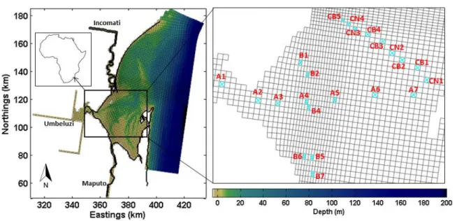
Mozambique is situated at the eastern coast of Africa, between 10° 27’ and 26° 52’ South and 30° 12’ and 40° 51’ East (see Figure 1).

Figure 1: Location and bathymetries of Maputo Bay a) Maputo Bay in a continental context (from Lencart e Silva, 2007), b) bathymetries of Maputo Bay and location of Maputo City.

(25)

9 In 2007, its population was estimated to be 17.2 million people, with an annual growth rate of

2.5 % (Hoguane, 2007). Mozambique has a coastline of approximately 2700 km, characterised by a large variety of ecosystems, including beaches, dune systems, coral reefs, mangrove swamps and estuaries (Canhanga, 2004; Sete et al., 2002).

Maputo Bay is located in the South of Mozambique with its centre at 32°47’ East 26°03’ South (Lencart e Silva, 2007). The bay covers a total area of approximately 1875 km2. In the North, it opens towards the Indian Ocean, whereas the East is limited by Machangulo Peninsula, Inhaca Island, Ilha dos Portugueses and several unvegetated islands in between, surrounded by shallow tidal channels and intertidal flats (Cooper and Pilkey, 2002). The city of Maputo is located on the western side and has a population of 2 million people (Sete, 2002). Water depths in the bay are on average around 5 m and reach approximately 30 m at the 18 km wide opening. An area of around 138 km2 is covered by sand banks (Hoguane, 1994) and the bay’s bottom is sandy in the eastern part and muddy in the western part (Canhanga, 2004). The bay is surrounded by mangrove swamps such as the Ponta Rasa mangrove swamp on Inhaca Island, 70% of which is covered by mangroves (Hoguane et al., 1999). The port of Maputo is located within the bay and is one of the three largest ports of Mozambique, being an important infrastructure for not only Mozambique but also the neighbouring countries such as South Africa and Swaziland (Canhanga, 2004; Hoguane, 2007). The port constitutes a possible source of pollution to the area, e.g. through oil, cleaning tanks and rubbish from boats.

The bay is also considered an important fishing ground due to the mangrove swamps and high productivity. The local population benefits from the collection and capture of fish, crabs and shellfish (De Boer and Longamane, 1996). Especially shrimp is an economically important resource for the area (Hoguane, 2007). Inhaca is also one of the most important tourism centres of Mozambique (Hoguane, 2007).

Due to the drainage of several international rivers into the bay, as well as the main industries of Mozambique located in the nearby areas and inadequate domestic waste treatment facilities for the large population of Maputo, the bay is prone to pollution (Sete et al., 2002). Hoguane (2007) describes five main pressures for Mozambique’s coastal zones, most of which are also relevant for the Maputo Bay area: coastal erosion, deforestation (especially of mangroves), deficiencies in the conservation of fish stocks, marine pollution and an inadequate distribution of energy, leading in turn to further deforestation due to increased use of biomass energy. Especially marine pollution can be a problem in Maputo Bay. Many cities in Mozambique have an incapacity to treat urban discharges appropriately, which leads to their discharge into the adjacent rivers and eventually reaching the bay.

2.2 Meteorologic Conditions

Average wind speeds are around 4 ms-1 and can therefore be characterised as relatively light, with sea breezes often developing in the afternoon (Lencart e Silva et al., 2010). Those authors therefore suggest that winds have a limited influence on the bay hydrodynamics, compared to the strong energy input from tidal forcing. Wind speeds at Mavalene airport station between March

(26)

2003 and April 2004 never exceeded 15 ms-1. Wind directions were mainly northward with less frequent W-E or SSW-NNE directions (Lencart e Silva, 2007).

The climate is between tropical and subtropical, with two pronounced seasons: wet season between October and March and dry season between April and September (Canhanga, 2004). The mean annual rainfall is 884 mm (de Boer et al., 2000).

Monthly average minimum and maximum temperatures for Maputo are shown in Table 1.

Table 1: Monthly average maximum and minimum air temperatures in Maputo (Climatemps, 2013).

Jan Feb Mar Apr May Jun Jul Aug Sep Oct Nov Dec

Max 30 30 30 29 27 25 25 26 27 28 28 30

Min 22 22 21 19 16 14 14 15 16 18 20 21

2.3 Hydrography and Hydrodynamics

Three main rivers flow into Maputo Bay: the Maputo, the Incomati and the smaller Umbeluzi (see Figure 1. The rivers Tembe and Matola also discharge in Maputo Bay but carry much smaller volumes of water. The Incomati makes up around 57 % of the freshwater discharge into the bay, being characterised by a mean discharge of 133 m3s-1. The Maputo River accounts for a further 38 % of runoff, with a long-term mean discharge of 89 m3s-1, whereas the remaining 5% of runoff come from the Umbeluzi River (Milliman and Meade, 1983). River discharge is characterised by a strong seasonal cycle, with maximum values usually occurring in the wet season between November and April, and reaching values exceeding 1000 m3s-1 during extreme events such as in a catastrophic flooding event with extreme rainfall in the year 2000 when peak discharges were up to 6827 m3s-1 (Lencart e Silva et al., 2010). Inter-annual discharge also shows strong variations, with a variation coefficient of 50-65 % for the Incomati River (Vas and v.d. Zaag, 2003). Since the 1960s, several dams have been built, influencing river runoff into Maputo Bay. Please refer to Vas and v.d. Zaag (2003) for an overview of all major dams of the Incomati basin.

The rivers are clearly influenced by the wet season – dry season cycle: both, the Umbeluzi and Maputo rivers have 67-82 % of their total runoff occurring between January and April and 37-52 % of the runoff occurring in the peak flood period in February and March (Sete et al., 2002). The total volume of fresh water entering the bay is estimated to be around 6 km3y-1 (Hoguane and Dove, 2000).

Sete et al. (2002) observed annual mean sea level variations in Maputo Bay, with maximum sea level coinciding with the wet season (January) and minimum values around 170 mm lower in the dry season (August). Those authors therefore conclude that intra annual sea level variations in Maputo Bay are influenced by rainfall or runoff in the river catchments flowing into the bay. Canhanga and Dias (2005) studied the tidal characteristics of Maputo Bay through the application of the numerical model SIMSYS2D and observations of free surface elevations in the harbour of Maputo Bay. They found that phases of M2 and S2 are 122° and 164°, respectively, and observed a

(27)

11 strong fortnightly modulation, indicating relatively large differences between spring and neap

tides, with spring tidal range being around 3 m and neap tidal range being just around 1 m. Those authors furthermore found that the semidiurnal M2 and S2 constituents contribute around 90 % of the total astronomical tide, whereas the amplitude of the K1 constituent is very small, being only 5% of the amplitude of the M2 constituent. Canhanga and Dias (2005) therefore suggest that constituents with an amplitude smaller than that of K1 may be neglected in the tidal analysis of Maputo Bay. Tidal amplitudes decrease inside the Bay, with M2 varying between 0.96 m at the mouth and 0.65 m inside the bay at the Espirito Santo Estuary, whereas the S2 amplitude varies between 0.47 and 0.32 m and the amplitude of K1 varies between 0.057 m and 0.045 m. The tidal phase increases towards the inshore zone, with the increase being more pronounced in smaller channels compared to the bay’s central part. The form factor

(1)

calculated from the amplitudes of the most important diurnal and semidiurnal constituents is smaller than 0.25 across the complete bay, mostly varying near values of around 0.06, confirming the semi-diurnal character of Maputo Bay. Maximum tidal currents are found in the main channel and are around 1 ms-1 and 0.5 ms-1 for M2 and S2, respectively. Taking into account the phase differences between free surface elevations and currents, the tide in Maputo behaves as a mixed wave, showing characteristics of both, a standing wave component and a progressive wave component. This mixed wave character was also observed by Lencart e Silva (2007), who concluded that the tide is close to a standing wave with only a small progressive component, indicated by a short lag between the bay’s mouth and locations further inside the bay.

Lencart e Silva et al. (2010) investigated the interactions between tidal stirring and the strongly varying river runoff in Maputo Bay, based on observations and the application of the three-dimensional hydrodynamic model Delft3D-flow. Their observations were in concordance with the previously observed dominance of semi-diurnal tidal constituents, with peak near-surface currents during spring tide being 1.2 ms-1 during flood and 1.0 ms-1 during ebb, while neap tide currents only reached velocities below 0.2 ms-1. This semi-diurnal characteristic can also be found in the energy dissipation per unit volume, which Lencart e Silva et al. (2010) calculated using

| ̅| (2)

where is the bottom drag coefficient, ρ is density of seawater, | ̅| is the magnitude of the tide-averaged depth mean tidal current magnitude and h is water depth. During spring tides, ε reaches approximately 0.1 Wm-3 over most of the bay, with a small area near Inhaca Island reaching 1.0 Wm-3, indicating pronounced mixing during spring tide. During neap tide, on the other hand, values of energy dissipation are two to three orders of magnitude smaller, indicating significantly lower levels of stirring. Tide lags between Clube Naval at the city of Maputo and Inhaca Island of 8 and 12 minutes, for M2 and S2, respectively, were found by Lencart e Silva (2007).

Lencart e Silva et al. (2010) observed bay-average salinities between 35.6 at the end of the dry season and 33.5 during the wet season, when freshwater input was largest. Bay-average water

(28)

temperatures varied between 21°C in July and 27.5°C in February, which lead to a stratifying effect due to the rate of heating of

( )

̇

(3)

where α is 104°C-1, cp is the specific heat and ̇ is the amplitude of the rate of heat exchange through the sea surface, defined as:

̇ (4)

where ω is the angular frequency of the annual cycle, ρ is the density of sea water and h is the water depth.

Those authors also compared this with the stirring effect: (

) | ̅|

₍₅₎ where e is the mixing efficiency and UM2+S2 is the tidal stream amplitude.

This shows that during spring tide stirring is much stronger than the stratifying effect from heating. During neap tide, stirring still meets the values of stratification from heating, even though tidal energy is much smaller. As stratification occurs and does not seem to be induced by heating, Lencart e Silva et al. (2010) conclude that the estuarine circulation and tidal straining effects must be responsible for the introduction of stratification.

Lencart e Silva (2007) calculated the stratifying effect of freshwater distributed uniformly at the surface for large river runoff:

(

) ̇

₍₆₎

where ̇ is the freshwater flow from rivers distributed as rainfall, s is the salinity and is the density difference between fresh and salt water (=25 kg.m-3).

Comparing the mean potential energy anomaly φ values throughout the year, Lencart e Silva et al. (2010) observed hardly any stratification during dry season and some stratification with φ values of around 1 Jm-3 during spring tides in the wet season. They further investigated the wet season stratification-stirring competition along a section of the bay between Inhaca Island and Macaneta sand spit. CTD measurements showed pronounced stratification during neap tide, especially in the deeper parts of the section, with φ ranging between 30 and 80 Jm-3, implying the stratifying effects of estuarine circulation dominating over mixing effects. During spring tide, the section was mixed for most of the tidal cycle, only showing little stratification in the deeper parts around low water, with φ reaching approximately 10 Jm-3 associated with larger velocity shear and therefore tidal straining. Wind stirring was found to be negligible compared to tidal stirring over most of the tidal cycle. Lencart e Silva et al. (2010) concluded that Maputo Bay’s large variation of freshwater input over the year leads to a vertical homogeneity of the water during the dry season and horizontal density gradients during the wet season due to the input of large amounts of fresh water.

(29)

13 Through the application of a three-dimensional hydrodynamic model, Lencart e Silva (2007)

investigated residual currents in Maputo Bay and found a flow into the bay through the deeper, south-eastern channel and an outward flow through the north-western, shallow areas, independent of tidal regime. These two separate flow cells cover the complete water depth of the bay during the dry season, with increased tidal forcing during spring tide leading to larger residual current velocities. During the wet season, spring tide conditions are similar but neap tide conditions are characterised by an estuarine circulation, with the deeper inward cell showing increased velocities while the area of outward flow expands towards the centre and top of the bay’s opening. Residual velocities for shallow water constituents were found, with velocities of 0.05 ms-1. Lencart e Silva (2007) assumes that these are due to tidal rectification, produced locally by the varying bathymetry over which the tidal currents propagate, as there was no evidence of these features in sea surface elevations. Furthermore did that author find the less intense vertical tidal mixing during neap tides leading to vertical gradients. These gradients in turn force a strong estuarine-type circulation, transporting surface water out of the bay and deeper, more dense water into the bay, thus increasing transport. During increased tidal mixing associated with spring tides, the water is vertically mixed, leading to an arrestment of the estuarine circulation and a retainment of much of the freshwater in the bay.

Lencart e Silva (2007) also applied different models to calculate the flushing time of Maputo Bay. A tidal prism model produced wet season mean flushing times of 9 and 17 days, for bay water return fractions of 0.8 and 0.9, respectively. Applying Delft3D-flow to Maputo Bay, that author found flushing times varying with freshwater input and tidal velocities, with a flushing time of 24 days during maximum river runoff and 37 days during no river runoff but with maximum tidal forcing. This indicates that Maputo Bay has a larger exchange efficiency when forced by buoyancy (fresh water from river discharge) than by tidal processes.

The freshwater discharge from the several estuaries leads to Maputo Bay being characterised by a gulf-type region of fresh water influence (ROFI), rather than a classic estuary. Simpson defines a ROFI as a “region between the shelf sea regime and the estuary where the local input of

freshwater buoyancy from the coastal source is comparable with, or exceeds, the seasonal input of buoyancy as heat which occurs all over the shelf” (1997).That author further argues that a

gulf-type ROFI is one in which the coastal topography retains the buoyancy input close to its source through constraining by topography. The exchange flow, exporting buoyancy, becomes similar to that of a classical estuarine circulation.

2.4 Regional Oceanographic Context

Saetre and Jorge Silva (1982) classified the water masses along the Mozambican coast up to a depth of 1000 m into four types: warm, low-salinity surface waters in the upper 100-150 m originating from the South Equatorial Current or the centre of the sub-tropical gyre of the Indian Ocean, sub-surface waters with a salinity maximum between 150 and 300 m depth, central water at a depth of 300-600 m and intermediate water of low salinity from the Antarctic or higher salinity water from the northern Indian Ocean.

(30)

Surface waters off the coast of southern Mozambique, near Maputo Bay, were found to be characterized by temperatures varying from a maximum of 26-29°C between January and March, to a minimum of 22-25°C between July and September. Surface salinities showed lowest values of 34.4-35.2 between January and March and maximum salinities of 35.3-35.5 occurring at the end of the dry season between October and November (Sete et al., 2002).

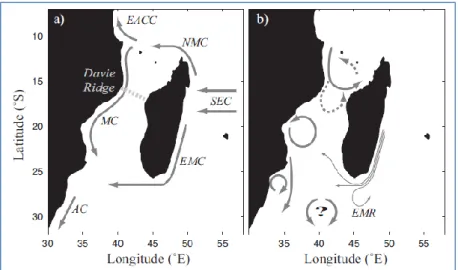
Lutjeharms and Jorge da Silva (1988) investigated the existence and characteristics of the cyclonic Delagoa Bight eddy, the Delagoa Bight being the shelf area adjacent to Maputo Bay. Through different sets of hydrographic data as well as sediment patterns they found that an eddy-like feature is located in the bight, covering most of the continental shelf as well as the terrace landward of the Mozambique Current. The feature has a high consistency, being found most or even all the time, and has a diameter of approximately 180 km. Those authors suggest the constriction of the shelf width at the Delagoa Bight causing the development of an upstream coastal countercurrent which forms the landward border of the Delagoa Bight lee eddy and advects warm water towards the North. Unlike in the surrounding areas, subtropical water is not found in the eddy. Instead, the core consists for a large extent of Antarctic Intermediate Water, upwelled from greater depths.

Quartly and Srokosz (2004) used chlorophyll concentrations obtained from satellite data to trace currents and eddies in the Southern Mozambique Channel through chlorophyll concentration fronts. Their results indicate that the previously assumed flow concept of the South Equatorial Current should be discarded. This previous concept consisted of the South Equatorial Current, when reaching Madagascar, dividing into a northward and a southward branch, the southward branch turning westward to feed into the Madagascar Current and forming the Argulhas Current. Instead, those authors suggest a more variable flow field. They found 200 km-diameter features with anticyclonic circulation travelling southward down the western side of the channel, 5-6 of which were observed per year. The Delagoa Bight eddy previously described by Lutjeharms and Jorge da Silva (1988) was confirmed and is expected to be enforced by anticyclonic eddies passing by seaward of the Delagoa Bight eddy. Furthermore were 250 km-diameter cyclonic eddies found near the Southern tip of Madagascar, which are assumed to originate further northward but only become apparent under the influence of the west of Madagascar, in the presence of coastal waters which are advected around the eddies. These eddies then travel west- to south-westward. A retroflecting East Madagascar Current was only found in some instances. Quartly and Srokosz’s findings are summarised in Figure 2, showing the long term mean flow (a) as well as varying features (b) of the Southern Mozambique Channel.

Significant wave heights in the high seas off Maputo Bay are between 7 and 11.7 m, with directions coming from mainly southern and eastern sides, whereas the waves in shallow water closer to the coast largely vary in height and direction (JIC Limited, 1998, in Hoguane, 2007).

(31)

15

Figure 2: Regional oceanographic context of Maputo Bay; a) long-term flow conditions, b) variability in features. Symbols: SEC: South Equatorial Current, NMC: North Madagascar Current, EACC: East African Coastal Current, EMC: East Madagascar Current, MC: Mozambique Current, AC: Argulhas Current, EMR: East Madagascar Retroflection. (Quartly and Srokosz, 2004).

3 Numerical Modelling

To investigate the hydrodynamics of Maputo Bay, the three-dimensional model Delft3D-flow was applied. This Chapter will introduce the methodology that was used. First, an overview of the hydrodynamic model and its features is given. Next, the model calibration and validation as well as the final model specifications are given. All scenarios that were applied are introduced and the limitations of the model are discussed. The data processing methods applied to transform the model output into the results is described.

3.1 Delft3D-flow

Delft3D-flow is a software for computations of coastal, estuarine and river areas and was developed by Deltares in the Netherlands. While the software Delft3D is able to carry out simulations for sediment transports, flows, waves, water quality, morphological developments and ecology, this chapter will only focus on the flow module, Delft3D-flow, used for this study. The model used in Delft3D-flow is based on the horizontal equations of motion, the continuity equation and the transport equations for conservative constituents. Various forcing mechanisms and other features are included and a range of options are given to define the horizontal and vertical coordinate systems, initial conditions, boundary conditions, friction, turbulence and other variables (Deltares, 2011).

Features

Delft3D-flow can be applied to both, two- and three-dimensional hydrodynamic modelling, being able to calculate transport phenomena and non-steady flow. Various forcing factors, including

(32)

tides, fresh-water discharge, wind, density stratification, thermal heating and cooling and Coriolis force can be taken into account.

The coordinate system can be Cartesian (in metres) or spherical (in decimal degrees). Horizontal grids in Delft3D-flow are staggered, meaning that the different quantities such as water levels, salinities and velocities are defined in different locations of the grid.

The particular staggered grid used in Delft3D-flow is the so-called Arakawa-C grid. In this grid, water level points are defined in grid centres, while velocities are defined perpendicular to the gird cell faces where they are situated. This approach has several advantages, such as an easier implementation of boundary conditions, the use of a smaller number of discrete state variables without losing accuracy, as well as preventing spatial oscillations in water levels (Deltares, 2011). For the vertical grid, up to 100 layers can be developed and each layer’s thickness can be specified. By giving layers non-uniform thickness, the resolution in areas of interest, such as the surface or bottom layer, as well as the pycnocline, can be improved.

A choice between the Z-model and the sigma-coordinate approach is given for the vertical grid direction (see Figure 3).

Figure 3: Comparison of the sigma-grid (left) and the Z-grid (right) (Deltares, 2011),

The sigma coordinate system is characterized by layers following the bottom topography and the free surface rather than layers being of uniform depth over the whole area. The number of layers is constant over the whole model domain. This approach therefore provides a refined vertical resolution in shallow areas (Deltares, 2011).

The σ co-ordinates are defined as:

(7)

where z is the vertical co-ordinate in physical space, ζ is the free surface elevation above the reference plane (z = 0), d is the depth below the reference plane and H is the total water depth (H = d + ζ).

(33)

17

Governing Equations

Delft3D solves the Navier-Stokes equations for incompressible fluids and considers the shallow water assumption as well as the Boussinesq assumption, taking into account variable density only in the pressure term (Deltares, 2011).

The system of equations therefore consists of the horizontal equations of motion, the continuity equation and the transport equations for conservative constituents.

Continuity Equation

The continuity equation is a mathematical statement of the conservation of mass (Officer, 1976). The depth-average continuity equation is given by

_√_√ [ ) √ √ √ [ ) √ (8) with ∫ ) (9)

being the contribution per unit area due to the withdrawal or discharge of water, with being the local sources of water, the local sinks of water, P being local precipitation, E the non-local evaporation and √ and √ being coefficients to transform values from curvilinear to rectangular coordinates (Deltares, 2011).

Horizontal momentum equations

The horizontal momentum equations in the u and v directions are defined as: _√ _√ _√_√ √ √ √ √ √ ) ( ) (10) and _√ _√ √ √ √ √ √ √ √ ) ( ) (11)

(34)

and represent forces due to an imbalance of horizontal Reynold’s stresses, and represent external sources and sinks of momentum and the vertical eddy viscosity coefficient is given by

) (12)

where is the kinematic viscosity of water, is the three-dimensional part of viscosity and _{is an ambient vertical mixing coefficient.}

The Coriolis parameter f is given by

(13)

and is dependent on the latitude and the Earth’s rotational speed. As the Boussinesq approximation is applied, density variations are only taken into account in the baroclinic pressure terms.

Vertical Velocities

The vertical velocity w can be obtained from the continuity equation (Equation 8) and is defined at the iso-σ-layer surfaces, representing the vertical velocity relative to the moving σ-plane (Deltares, 2011). _√_√ [ ) √ √ √ [ ) √ ) (14)

Hydrostatic Pressure Assumption

In areas where the depth is assumed to be much smaller than the horizontal length scale, vertical accelerations are considered to be small compared to gravitational acceleration and can therefore be neglected. In this case, the shallow water assumption is valid and the vertical momentum equation can be reduced to the hydrostatic pressure relation, not taking into account effects of sudden variation of bottom topography on vertical accelerations due to buoyancy variations, so:

(15)

After integration, the hydrostatic pressure assumption becomes:

∫ ) (16)

where Patm is the atmospheric pressure.

Considering water of uniform density, the pressure gradients in the ξ and η direction are given by

√ √ _√ (17) and

(35)

19 √ √ _√ (18)

and represent the barotropic pressure gradients. Atmospheric pressure is included for storm surge events (Deltares, 2011). If the density is assumed to be non-uniform, the baroclinic term of the pressure gradient must be taken into account and equations (17) and (18) become:

√ √ √ ∫ ( ) (19) and √ √ √ ∫ ( ) (20)

where the first two terms on the right are due to barotropic forcing, while the third term represents the baroclinic component due to non-uniform density (Deltares, 2011).

Transport equation

The transport of dissolved substances, heat or salinity in Delft3D-flow is expressed by a three-dimensional advection-diffusion equation. In a conservative form, with σ co-ordinates in the vertical and orthogonal curvilinear co-ordinates in the horizontal direction, the transport equation can be expressed by:

) _{√ √}, [√ ) [√ ) - √ √ , ( √ √ ) ( √ √ ( ) ) (21)

where and are the vertical and horizontal diffusion coefficients, respectively, is a first-order decay process and S represents the sources and sinks due to exchange of heat at the free surface and discharge and withdrawal of water (Deltares, 2011).

Boundary Conditions

The boundary conditions describe the influence of the outer world on the model area. This chapter will explain the flow boundary condition as well as the transport boundary conditions.

Flow boundary conditions

Concerning vertical flow boundary conditions, the water surface and bottom are assumed to be impermeable, not allowing any flow:

| | (22)

The boundary conditions for the momentum equations at the sea bed in the ξ and η directions are defined by: