1 2 3 4 5 6 7 8 9 10 11 12 13 14 15 16 17 18 19 20 21 22 23 24 25 26 27 28 29 30 31 32 33 34 35 36 37 38 39 40 41 42 43 44 45 46 47 48 49 50 51 52 53 54 55 56 57 58 59 60 61 62 63 64 65 1
Spatial distribution patterns and movements of Holothuria arguinensis in the Ria
1
Formosa (Portugal).
2 3
Andjin Siegenthaler a,b, Fernando Cánovas a, Mercedes González-Wangüemerta,* 4
5 6
a
Centro de Ciencias do Mar (CCMAR), CIMAR - Laboratório Associado Faculdade 7
de Ciências e Tecnologia (F.C.T.), Universidade do Algarve 8
b
University of Salford, School of Environment and Life Sciences
9 * Corresponding author 10 [email protected] 11
Centro de Ciencias do Mar (CCMAR), CIMAR - Laboratório Associado Faculdade de 12
Ciências e Tecnologia (F.C.T.), Universidade do Algarve, Campus de Gambelas P-13 8005-139 Faro, Portugal 14 Tel: (351) 289 800 900 (ext. 7408) 15 Fax: (351) 289 818 353 16 17 18 19 20 21 22 23 24 25 26 *Manuscript
Click here to view linked References
© 2015. This manuscript version is made available under the Elsevier user license
1 2 3 4 5 6 7 8 9 10 11 12 13 14 15 16 17 18 19 20 21 22 23 24 25 26 27 28 29 30 31 32 33 34 35 36 37 38 39 40 41 42 43 44 45 46 47 48 49 50 51 52 53 54 55 56 57 58 59 60 Abstract 1 2
Holothurian populations are under pressure worldwide because of increasing demand 3
for beche-de-mer, mainly for Asian consumption. Importations to this area from new 4
temperate fishing grounds provide economic opportunities but also raise concerns 5
regarding future over-exploitation. Studies on the habitat preferences and movements 6
of sea cucumbers are important for the management of sea cucumber stocks and 7
sizing of no-take zones, but information on the ecology and behaviour of temperate 8
sea cucumbers is scarce. This study describes the small-scale distribution and 9
movement patterns of Holothuria arguinensis in the intertidal zone of the Ria 10
Formosa national park (Portugal). Mark/recapture studies were performed to record 11
their movements over time on different habitats (sand and seagrass). H. arguinensis 12
preferred seagrass habitats and did not show a size or life stage-related spatial 13
segregation. Its density was 563 ind ha-1 and mean movement speed was 10 m per 14
day. Movement speed did not differ between habitats and the direction of movement 15
was offshore during the day and shoreward during the night. Median home range size 16
was 35 m2 and overlap among home ranges was 84 %. Holothuria arguinensis’ high 17
abundance, close association with seagrass and easy catchability in the intertidal zone, 18
indicate the importance of including intertidal lagoons in future studies on temperate 19
sea cucumber ecology since those systems might require different management 20
strategies than fully submerged habitats. 21
22 23 24 25
1 2 3 4 5 6 7 8 9 10 11 12 13 14 15 16 17 18 19 20 21 22 23 24 25 26 27 28 29 30 31 32 33 34 35 36 37 38 39 40 41 42 43 44 45 46 47 48 49 50 51 52 53 54 55 56 57 58 59 60 61 62 63 64 65 3 1. Introduction 1
Increasing demand of beche-de-mer is influencing sea cucumber populations all 2
over the world. The traditional Asian demand of holothurian products for delicacies 3
and medicines has resulted in the depletion of traditional fishing grounds in tropical 4
areas. The fishing pressure is now moving towards temperate areas, including the 5
Mediterranean Sea and Northeastern Atlantic Ocean (González-Wangüemert et al.,
6
2013, 2014, 2015; Toral-Granda et al., 2008). Nowadays, global catch estimates are in 7
the range of 100, 000 tonnes of sea cucumbers per year (Purcell et al., 2010). 8
9
The overfishing of sea cucumbers in the Indo-Pacific, has resulted in catch of
10
new target species (Holothuria tubulosa, H. polii, H. mammata, H. forskali and H.
11
arguinensis) from Mediterranean Sea and NE Atlantic Ocean (Aydin, 2008; 12
González-Wangüemert et al., 2014; González-Wangüemert and Borrero-Pérez, 2012;
13
Rodrigues et al., 2015; Sicuro and Levine, 2011). In the last three years, the sea
14
cucumber fishery in Northern Turkey has increased rapidly, with 555 Tn in 2011
15
(80% H. polii and 20% H. tubulosa plus H. mammata) (González-Wangüemert et al.,
16
2014). Sea cucumbers are fished by hookah facilities, a diver catches around
2.000-17
3.000 individuals per day (Aydin, 2008); the current Turkish fleet (120 vessels) can
18
collect around 720.000 sea cucumbers per day (González-Wangüemert et al., 2014).
19
As consequence, some signals of over-exploitation were already detected, showing
20
loss of the largest and heaviest individuals and genetic diversity
(González-21
Wangüemert et al. 2015). Scarce official information on sea cucumber fisheries from
22
this geographical area is available due to catches are catalogued as “invertebrates”
23
and/or obtained illegally. In Spain, more than 10 companies are exporting sea
24
cucumbers to China
1 2 3 4 5 6 7 8 9 10 11 12 13 14 15 16 17 18 19 20 21 22 23 24 25 26 27 28 29 30 31 32 33 34 35 36 37 38 39 40 41 42 43 44 45 46 47 48 49 50 51 52 53 54 55 56 57 58 59 60
supplier.html); some of them with 1-2 millions $ US of total revenue. The main target
1
species are H. tubulosa, H. forskali and H. mammata. In Portugal, three companies are
2
selling sea cucumbers, mainly Holothuria arguinensis, H. forskali and H. mammata,
3
offering supply ability among 2.000-50.000 Kg/month and prices oscillating among
4
70-350 euro/kg (http://www.alibaba.com/countrysearch/PT/sea-cucumber.html)
5
depending on quality of product.
6 7
Holothurians are sensitive to over-exploitation due to a combination of biological 8
(late maturity, low recruitment rate and density-dependent reproduction), and 9
anthropogenic factors (the ease with which shallow water species can be harvested) 10
(Bruckner et al., 2003). Dramatic reductions in sea cucumber abundance might cause 11
concern about their ecological role in bioturbation, nutrient recycling and habitat 12
structuring (Bruckner et al., 2003; Uthicke, 1999, 2001a, b), and also on the food-13
web, because sea cucumbers are a substantial biomass for some predators as fishes, 14
starfishes and crustaceans (Francour, 1997). 15
16
Information on the ecology and behaviour of sea cucumbers is relatively scarce 17
(Bruckner et al., 2003; Conand, 1990; Graham and Battaglene, 2004; Navarro et al., 18
2013, 2014), despite their economical and ecological importance. Studies on the 19
habitat preferences and movements of sea cucumbers have demonstrated their utility 20
on the management of sea cucumber stocks and sizing of no-take zones providing for
21
example, parameters for surveys and restocking (Purcell and Kirby, 2006; Shiell and 22
Knott, 2008). 23
1 2 3 4 5 6 7 8 9 10 11 12 13 14 15 16 17 18 19 20 21 22 23 24 25 26 27 28 29 30 31 32 33 34 35 36 37 38 39 40 41 42 43 44 45 46 47 48 49 50 51 52 53 54 55 56 57 58 59 60 61 62 63 64 65 5 Movement and distribution of sea cucumber can be influenced by several factors 1
such as substrate type, organic matter availability, light intensity, depth and salinity 2
(Dong et al., 2011; Hamel et al., 2001; Mercier et al., 2000; Navarro et al., 2013, 3
2014; Shiell and Knott, 2008; Slater et al., 2011). Movement speed is slow with
4
averages of 2-5 m day-1 for Holothuria fuscogilva, Holothuria whitmaei, 5
Apostichopus japonicus and Actinopyga mauritiana (Graham and Battaglene, 2004;
6
Reichenbach, 1999; Shiell, 2006; YSFRI, 1991) and around 10 m day-1 for Holothuria 7
sanctori (Navarro et al., 2013).
8 9
Behavioural studies on sea cucumbers are focused mainly on tropical species 10
(e.g. Graham and Battaglene, 2004; Mercier et al., 2000; Purcell and Kirby, 2006; 11
Reichenbach, 1999; Shiell, 2006; Shiell and Knott, 2008), but information on 12
temperate species is still scarce (Navarro et al., 2014). 13
14
Holothuria arguinensis is a sea cucumber that is distributed along the east North
15
Atlantic from Portugal to Morocco, Mauritania and Canary Islands (González-16
Wangüemert and Borrero-Pérez, 2012; Rodrigues, 2012), and some individuals have 17
been found in the Mediterranean sea on the south-eastern Spanish coast recently 18
(González-Wangüemert and Borrero-Pérez, 2012). This species is usually associated 19
with sandy/rocky areas and seagrass meadows where it occurs from 0 m to 50 m depth 20
(González-Wangüemert and Borrero-Pérez, 2012; Navarro, 2012; Rodrigues et al., 21
2015). In Ria Formosa National Park (South Portugal) this species is the most 22
abundant holothurian and can be found in high densities exposed on the intertidal flats 23
during low tide (González-Wangüemert et al., 2013). As was stressed before, H.
24
arguinensis is one of the target species caught in Portugal to be exported mainly to 25
1 2 3 4 5 6 7 8 9 10 11 12 13 14 15 16 17 18 19 20 21 22 23 24 25 26 27 28 29 30 31 32 33 34 35 36 37 38 39 40 41 42 43 44 45 46 47 48 49 50 51 52 53 54 55 56 57 58 59 60
Asiatic countries. Nowadays, unless three companies are offering this species to be
1
sold (http://www.alibaba.com/countrysearch/PT/sea-cucumber.html). The
2
combination of its high nutritional value for human consumption (Roggatz, 2012), 3
high densities of its populations and the ease with which this species can be harvested, 4
makes it vulnerable to overexploitation such as another tropical species (Bruckner et 5
al., 2003). 6
7
The ecology and behaviour of H. arguinensis have been studied recently but only 8
on the Canary Islands (Spain), where this species is occupying habitats dominated by 9
volcanic rocks and seagrass at 4-8m depth (Navarro, 2012; Navarro et al., 2013, 2014; 10
Tuya et al., 2006). These habitats are substantially different from the tidal lagoon 11
habitat of Ria Formosa national park, where only one study on H. arguinensis has 12
been conducted to assess the population status of this species through a volunteer 13
program doing visual census (González-Wangüemert et al., 2013). We aim to study 14
the behaviour of H. arguinensis at small spatial scale in Ria Formosa Natural Park 15
(South Portugal). To achieve this objective, we analysed the movement patterns of H. 16
arguinensis, interpreted its spatial distribution across habitat-diverse areas, studied the
17
home-range of this species and its relationship with the size of individuals, and 18
estimated its density. This information would be very useful to further development of
19
regulations to sea cucumber fishery in Ria Formosa (Natural Park, South Portugal)
20
and along Portuguese coast. Also, these data have a valuable interest to develop the
21
aquaculture biotechnology on H. arguinensis, which could supply part of the demand
22
from Asiatic countries, with less impact on wild populations, and allow further
23
restocking programs if they are necessary.
1 2 3 4 5 6 7 8 9 10 11 12 13 14 15 16 17 18 19 20 21 22 23 24 25 26 27 28 29 30 31 32 33 34 35 36 37 38 39 40 41 42 43 44 45 46 47 48 49 50 51 52 53 54 55 56 57 58 59 60 61 62 63 64 65 7
2. Material and Methods
1
2.1. Study area
2
Ria Formosa Natural Park is a tidal lagoon, consisting of tidal flats and salt 3
marshes protected by a belt of dunes extending for 55 km along the south coast of 4
Portugal (Sprung, 1994). Total surface of the lagoon is about 10 000 ha and the 5
average depth is 3-4 m with a tidal amplitude of about 1.30 m at neap tide and 2.80 m 6
at spring tide. Channels are up to 20 m deep (Malaquias and Sprung, 2005; Sprung, 7
2001). Habitats are covered mainly by either sand, mud and seagrass (intertidal: 8
Zostera noltii, subtidal: Zostera marina, Cymodocea nodosa (Malaquias and Sprung,
9
2005)). Z. noltii biomass is high in the intertidal, showing low oscillations during the 10
year (Asmus et al., 2000). Sandy habitats are generally associated with intertidal 11
seaweed communities, consisting mainly on Ulva spp. and Enteromorpha spp. 12
(Asmus et al., 2000). 13
14
Experiments were carried out in the intertidal zone of the Ria Formosa close to 15
Praia de Faro (Fig. 1), covering an area along the coast from the high shore level to 16
the end of the intertidal zone. The area was selected because of its high holothurian 17
abundance (González-Wangüemert et al., 2013). Transects (60 m of length each one
18
and parallel to the waterline) were walked during periods of aerial exposure and
19
percentage of coverage by either seagrass, seaweed and sand were estimated for every
20
cell in a 1 m2 grid of the study area. Transects were separated 2 meters from each
21
other and the observer recorded at both sides of the transects for 1 m distance.
22
Although quadrants were not used for coverage estimates, the observer error was
23
minimized by the use of only one sampler. A principal component analysis (PCA)
24
was then used to summarize habitat variability across the study area by using spatial
1 2 3 4 5 6 7 8 9 10 11 12 13 14 15 16 17 18 19 20 21 22 23 24 25 26 27 28 29 30 31 32 33 34 35 36 37 38 39 40 41 42 43 44 45 46 47 48 49 50 51 52 53 54 55 56 57 58 59 60
distribution of coverage information already described above. Each cell of the study
1
area, can be then classified, interpreting the first component of the ordination.
2
Analysis was performed using GRASS GIS v.6.4.2 (Neteler et al., 2012), and
3
variables were represented by 1x1 m raster maps of each coverage type.
4 5
2.2. Mark/recapture experimental designing
6
A preliminary study was done and the methods retained were used in order to
7
optimize the sampling design. The study was performed during two periods at the 8
beginning and end of April 2013. Captures were made during periods of aerial
9
exposure (between 2 hours before low tide and 1 hour after low tide)for 5 consecutive 10
days (10 low tides per period). Tidal height at low tide varied from 0.57 to 0.70 m
11
(first period) and 0.36 to 0.60 m (second period) (Instituto Hidrográfico:
12
http://www.hidrografico.pt/previsao-mares.php). During each sampling, the whole
13
study area was searched and all holothurians encountered were marked in situ and
14
immediately released at the same spot where captured. Marking was done by
15
scratching a code on their dorsal surface with a surgical scalpel (Mercier et al., 2000;
16
Navarro et al., 2013, 2014; Reichenbach, 1999). The wound usually heals within 10
17
days, leaving a scar with the shape of the mark (Shiell, 2006; Supplementary Fig. S1).
18
Scratched marks are visible up to a month with no indication of any considerable
19
behavioural change (Mercier et al., 2000; Reichenbach, 1999). Other tagging methods 20
such as glued tags, colouring agents, PIT tags and T-bar tags were considered less 21
effective and often more invasive (Conand, 1990; Kirshenbaum et al., 2006; Navarro
22
et al., 2014; Purcell et al., 2008; Schiell, 2006). Stress caused by handling and
23
marking could result in a higher activity during the initial hours (Shiell, 2006).
24
Reducing this effect by postponing the sampling for several hours after marking
1 2 3 4 5 6 7 8 9 10 11 12 13 14 15 16 17 18 19 20 21 22 23 24 25 26 27 28 29 30 31 32 33 34 35 36 37 38 39 40 41 42 43 44 45 46 47 48 49 50 51 52 53 54 55 56 57 58 59 60 61 62 63 64 65 9
(Navarro et al., 2013, 2014), was not deemed effective since the specimens were also
1
handled during recaptures in those cases where the marks were difficult to read
2
directly. Observations started directly after marking and the effect of handling was
3
reduced by working in situ (Navarro et al., 2014). Recaptured individuals were 4
directly released without remarking since repeated marking could increase the chance
5
of infections and possibly behavioural changes. In the few cases that remarking was
6
essential to maintain the readability of the mark (12 % of the animals recaptured were
7
remarked once) the animals did not show a behavioural change. Total length, date, 8
time, substrate, and relative position (see positioning section for further explanations), 9
were recorded for every capture and recapture. The length was measured by metric
10
tape at the moment of capture in order to prevent underestimations because of 11
unpredictable contractions and evacuations of water (Hammond, 1982; Reichenbach, 12
1999). Temperature and salinity were measured twice per low tide with an Eutech Salt 13 6+ Salinity/temperature meter. 14 15 2.3. Positioning system 16
Reference position of an holothuria was estimated using the bearings relative to 17
two fixed reference marks and applying linear trigonometric functions. Those 18
references were placed at the shoreward corners of the study area. Angles were 19
measured using the geographical north as zero reference, using a Topomarine Rescue 20
7x50 waterproof/floating binocular with internal compass. Flash lights were used at 21
night to show the exact location of the captures. Angles were corrected for magnetic 22
declinations for the study area during the sampling days (2.57º W) and magnetic 23
deviations of the compass used prior to the calculations. Linear increment between 24
angles in magnetic deviations was assumed. 25
1 2 3 4 5 6 7 8 9 10 11 12 13 14 15 16 17 18 19 20 21 22 23 24 25 26 27 28 29 30 31 32 33 34 35 36 37 38 39 40 41 42 43 44 45 46 47 48 49 50 51 52 53 54 55 56 57 58 59 60 1
Geographical coordinates of reference marks were located using a Garmin 2
GPSmap 60CSx (European Terrestrial Reference System ETRS 1989 Datum, GRS 3
1980 spheroid, Transverse Mercator projection). Relative position of every specimen 4
was then corrected by using the reference mark absolute positions. All calculations 5
were done in R statistical software v.2.15.3 (R Development Core Team, 2013). 6
7
2.4. Data analyses
8
Size distribution was estimated from the dataset, which contained the length of 9
all captured individuals. Shapiro-Wilk test was then applied to test for normality. 10
11
To estimate the holothurian density within the study area, capture-recapture data 12
were encoded in absence/presence from the capture history, consisting on ones 13
(captures) and zeros (misses). Population size was estimated by fitting several models, 14
assuming a closed population (no migrants) due to the relatively slow-motion lifestyle 15
of the species and the short duration of the study (Baillargeon and Rivest, 2007). 16
Model selection was based on a combination of minimizing Akaike information 17
criteria (AIC) and standard error. The final abundance was estimated using profile 18
likelihood confidence intervals based on log-linear distribution with the closest fit. 19
20
Capture data was used to study habitat preferences. A grid (3 x 3 m cells) of the 21
study area was used to summarize the capture data, allowing to analyse habitat 22
preferences independently of the number of recaptures, and later test for differences 23
between habitats for both presence of individuals and size. A total of 125 cells 24
covered the seagrass area (>74% seagrass, < 5% sand) and 210 cells covered the 25
1 2 3 4 5 6 7 8 9 10 11 12 13 14 15 16 17 18 19 20 21 22 23 24 25 26 27 28 29 30 31 32 33 34 35 36 37 38 39 40 41 42 43 44 45 46 47 48 49 50 51 52 53 54 55 56 57 58 59 60 61 62 63 64 65 1 1 sandy area (>74/% sand, < 5% seagrass). 23 cells covered the transition area between 1
seagrass and sand but were not considered due to their low abundance. Cells were 2
considered sampling units and independent from each other. 50 cells per habitat and 3
tidal cycle were randomly selected and a generalized linear model (GLM) with a 4
binomial distribution was applied to test for differences in presence/absence between 5
the habitats. Average length per cell was also calculated for all cells containing any 6
individual. One-way ANOVA was used by implementing a sequential sum of squares
7
(type I) to compare length distribution using as factors “periods” and “habitat”.
8 9
Movement speeds were only calculated for recaptures between consecutive
10
tides and within the same habitat. Mean movement speed was biased towards higher
11
values due to infrequent movements over longer distances, possibly influenced by the
12
currents and the behavioural effects of marking (Navarro et al., 2013, 2014). Because
13
of this skewed distribution, median speed for each individual was used. Differences in 14
median movement speeds between habitats were then compared using one-way 15
ANOVA, also considering differences between the two periods. Pearson correlation 16
coefficient was used to explore the relationships between the individual length and 17
movement speed. 18
19
Orientation of movement was tested on the dataset, containing all time intervals
20
and independent of the number of recaptures. Angles were transformed into circular 21
and Rayleigh test for randomness was applied. Circular one-way ANOVA was then 22
used to test for differences in orientation between periods, habitats and day/night 23
group of means, under the null hypothesis of same mean direction for all the group 24
1 2 3 4 5 6 7 8 9 10 11 12 13 14 15 16 17 18 19 20 21 22 23 24 25 26 27 28 29 30 31 32 33 34 35 36 37 38 39 40 41 42 43 44 45 46 47 48 49 50 51 52 53 54 55 56 57 58 59 60
means (See: Lund and Agostinelli, 2013). Circular Pearson test for correlation was 1
also used to explore the relationships with wind direction. 2
3
Movement patterns and home ranges were analysed by specimen which was 4
recaptured for a minimum of 4 times within one period (movement patterns) or over 5
both periods (home ranges). Movement patterns were described based on visual 6
analysis of the data plotted on the habitat map and on linearity indices (net distance
7
travelled/gross distance). Differences in occurrence of specific movement patterns 8
between the two periods were tested using a binominal test for the movement patterns 9
and a Mann-Whitney U test for the linearity indices. The minimum area method 10
(which is based on the smallest area convex polygon that contains all capture points)
11
was applied for the calculation of the home range area (Worton, 1987). 12
13
All analyses were done in R statistial software v.2.15.3, using packages 14
“Rcapture” (Baillargeon and Rivest, 2012), which estimates parameters in capture-15
recapture experiments by the use of Poisson regressions (Baillargeon and Rivest, 16
2012), and “circular” (Lund and Agostinelli, 2013), which allows to manage angular 17
data. Data met the normality and homoscedasticity requirement of ANOVA. Home 18
range area and overlap between home ranges were calculated using GRASS GIS 19
v.6.4.2 (Neteler et al., 2012) and visualized in Quantum GIS v.1.8.0 (Quantum GIS 20
Development Team, 2009). 21
1 2 3 4 5 6 7 8 9 10 11 12 13 14 15 16 17 18 19 20 21 22 23 24 25 26 27 28 29 30 31 32 33 34 35 36 37 38 39 40 41 42 43 44 45 46 47 48 49 50 51 52 53 54 55 56 57 58 59 60 61 62 63 64 65 1 3 3. Results 1 3.1. Habitat description 2
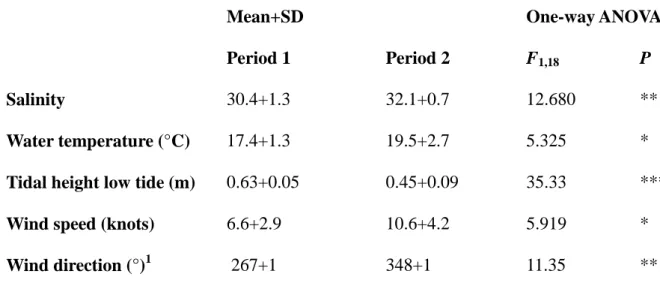
The two study periods (8-12 April and 24-28 April 2013) differed significantly 3
in hydrological conditions (Table 1). During the second period, the water was warmer 4
and saltier, and the wind speed was higher than during the first one. The wind blew 5
mainly from the West during the first period and from the North-North-West during 6
the second one. Tidal height of low tide was higher during the first period. 7
8
The study area can be divided in two mayor habitats which were dominated by 9
sand (44.5 % coverage) or seagrass (35.6 % coverage). Seaweeds covered 19.9 % of 10
the area and generally occurred in the sandy habitat (Fig. 2A-C). The first component 11
of the PCA explains 83.25 % of the variance for the habitat composition (Fig. 2D). 12
Seagrasses were found in the North to North-East half of the study area and consisted 13
of two patches that were separated by a sandy channel of 1-4 m wide. The sandy 14
channel between the two seagrass patches recorded the same depth as the patches. 15
Stronger currents were observed within the channel compared to the other areas 16
during the upcoming and retreating tides. 17
3.2. Abundance and length
18
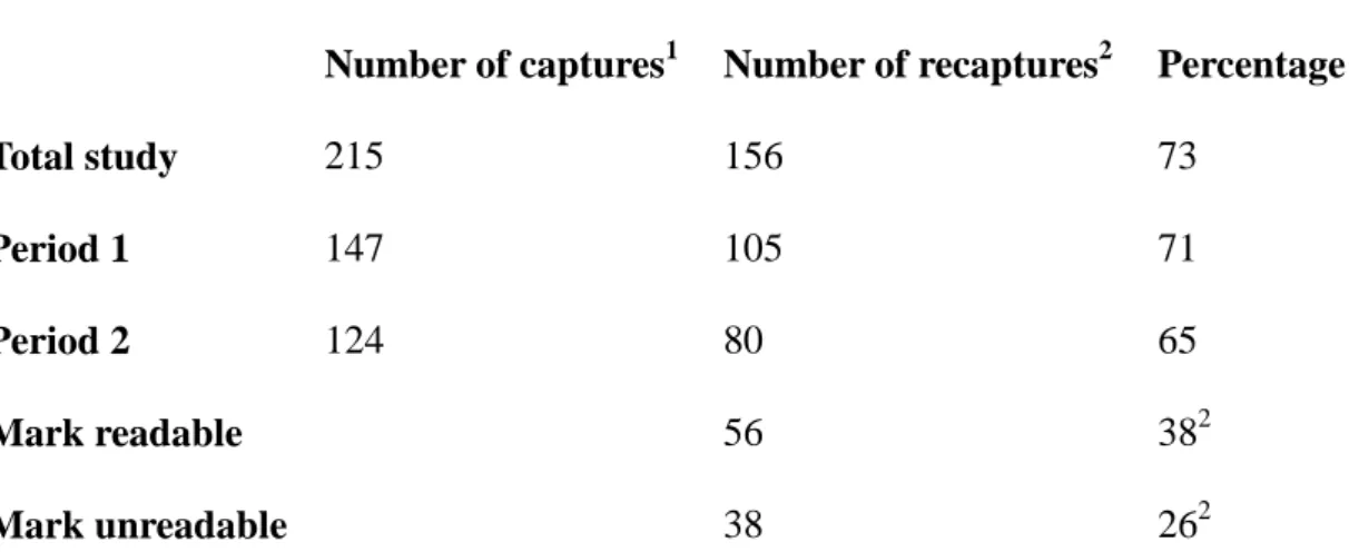
A total of 215 specimens of H. arguinensis were captured during this study with 19
an average recapture probability of 73 % (Table 2). A small difference of 6 % in 20
recapture probability was observed between the periods. 63 % of individuals which 21
were caught during the second period, showed marks from being captured during the 22
first period, but only 38% of the recaptures had a readable code. The Mh Chao (LB) 23
and Mth Darroch models for population size estimation were selected based on AIC. 24
Estimated numbers of H. arguinensis within the study area were 169 individuals (CI: 25
1 2 3 4 5 6 7 8 9 10 11 12 13 14 15 16 17 18 19 20 21 22 23 24 25 26 27 28 29 30 31 32 33 34 35 36 37 38 39 40 41 42 43 44 45 46 47 48 49 50 51 52 53 54 55 56 57 58 59 60
155-193) and 158 individuals (CI: 141-184), for period 1 and 2 respectively. Total 1
density estimates range from 527-563 individuals ha-1. Differences in presence
2
between both seagrass (average number of cells present = 9) and sand (average
3
number of cells present = 1) habitats, were significant (binomial GLM: Z1799 = 9.338, 4
P < 0.001). Differences between average numbers of presences between periods 5
(period 1 = 10, period 2 = 10; binomial GLM: Z1799 = -0.618, P = 0.537) and between 6
day and night (day = 11, night = 9; binomial GLM: Z1799 = -1.129, P = 0.259), were 7
not significant.
8
Length distribution of all captured H. arguinensis specimens showed a Gaussian 9
distribution (Shapiro-Wilk normality test: X+SD = 20+5 cm, W = 0.9921, N = 225, P 10
= 0.2702). Mean length differed slightly but significantly between the two periods 11
(Period 1: X+SE = 22+0.4 cm; Period 2: X+SE = 20+0.5; ANOVA: F1,273 = 13.55, P < 12
0.001). This difference was not considered for further analysis, since the differences 13
between the means were so small that they felt within the natural variation of 14
contraction of the specimen. Mean length per cell did not differ between the habitats 15
(ANOVA: F1,497 = 2.30, P = 0.13). 16
17
3.3. Movement patterns and home ranges
18
Median (X+SE) movement speed of H. arguinensis was 0.42+0.37 mh-1, and 19
did not differ between periods (ANOVA: F1,89 = 1.948, P = 0.166) nor habitats 20
(ANOVA: F1,89 = 0.024, P = 0.877). Length and movement speed were independent 21
and uncorrelated (Pearson correlation: rp = 0.07, N = 102, P = 0.50), as well as 22
movement speed between night and day (Paired samples T-test with log-23
transformation: t51 = -1.79, P = 0.08). 24
1 2 3 4 5 6 7 8 9 10 11 12 13 14 15 16 17 18 19 20 21 22 23 24 25 26 27 28 29 30 31 32 33 34 35 36 37 38 39 40 41 42 43 44 45 46 47 48 49 50 51 52 53 54 55 56 57 58 59 60 61 62 63 64 65 1 5 Directionality of movements differed significantly between day and night 1
(Circular ANOVA: F1,328 = 376.8, P < 0.001; Fig. 3). Movements during the day were 2
not random (Rayleigh test: Z = 0.325, N = 217, P < 0.001) and orientated towards the 3
NNE (X+SD = 12.7+1.5°). Movements during the night were also not random 4
(Rayleigh test: Z = 0.375, N = 113, P < 0.001) but were orientated in the opposite 5
direction, the SSW (X+SD = 205.1+1.4°). Directionality was not correlated with wind 6
direction (circular Pearson correlation: rp = -0.92, N = 377, P = 0.36). Animals 7
captured in both seagrass and sand habitats moved in NE (offshore) direction 8
(Circular ANOVA: F1,215 = 1.831, P = 0.178; Fig. 3) during the day, and in SW (near 9
shore) direction during the night (Circular ANOVA: F1,111 = 3.719, P = 0.056). 10
11
Several movement patterns were observed on H. arguinensis during this study
12
(See supplementary Fig. S2 for a representation these patterns). The two most 13
abundant patterns were directional (without showing a preference for a certain area;
14
Nperiod 1 = 14; Nperiod 2 = 3) and clustered movements (showing a preference for a 15
certain area in which recaptures do not show a directional movement but are
16
clustered; Nperiod 1 = 1; Nperiod 2 = 15). Variations on directional movement were also 17
observed: semicircular (directional towards the starting point; Nperiod 1 = 4; Nperiod 2 = 18
1) and zigzag (limited directionality and covering more area on the way; Nperiod 1 = 6; 19
Nperiod 2 = 3). A combination of directional and clustered movement was observed 20
regularly where the specimen showed directional movement towards or from an area
21
where it clustered (Nperiod 1 = 12; Nperiod 2 = 10). H. arguinensis showed significantly 22
more directional movement during the first period than during the second (Binomial
23
test: N = 17, P = 0.013) and more clustered patterns during the second than during the
24
first one (Binomial test: N = 16, P < 0.001). The ratio net distance travelled (X+SE =
1 2 3 4 5 6 7 8 9 10 11 12 13 14 15 16 17 18 19 20 21 22 23 24 25 26 27 28 29 30 31 32 33 34 35 36 37 38 39 40 41 42 43 44 45 46 47 48 49 50 51 52 53 54 55 56 57 58 59 60
Period 1: 11.5 + 1.0 m; Period 2: 5.3 + 0.6 m) per gross distance (X+SE = Period 1:
1
27.2 + 2.8 m; Period 2: 18.3 + 1.8 m) was significantly higher during the first period
2
than during the second (Period 1: 0.56 + 0.03 m ; Period 2: 0.33 + 0.04 m;
Mann-3
Whitney U test: Z25,31 = -2.810, P < 0.01). 4
5
Home ranges of H. arguinensis are shown in Fig. 4. Median (+SE) home range 6
area was 35+10 m2. On average, 84 % of each home range was overlapped. As visible 7
in Fig. 5, the sandy channel between the seagrass patches was included in most of the 8
home ranges. No correlation between the individual size and the home range area was 9
observed (Pearson correlation: rp = 0.10, N = 69, P = 0.40). 10
11
4. Discussion
12
The results of this study provide a valuable insight in the small scale distribution 13
of H. arguinensis. Estimated densities of 527-563 ind. ha-1 are slightly higher than H. 14
arguinensis’ densities of ca. 250 (seagrass meadow) and 460 (macroalgal bed) ind. ha -15
1
measured on the Canary Islands by Navarro et al. (2012; 2014). Although the
16
differences between studies could be also due to other locational differences than
17
habitat type, these results clearly indicatethe importance of intertidal lagoons such as
18
the Ria Formosa for this species. Holothurian density varies per location within the 19
Ria Formosa (González-Wangüemert et al., 2013) and the estimates of the present 20
study are in line with the highest densities measured by those authors. 21
22
H. arguinensis shows a preference for the seagrass habitat over the sandy habitat. 23
This result should, however, be considered with care since its preference could be
24
confounded with tidal elevation. Nevertheless, the results of this study agree with
1 2 3 4 5 6 7 8 9 10 11 12 13 14 15 16 17 18 19 20 21 22 23 24 25 26 27 28 29 30 31 32 33 34 35 36 37 38 39 40 41 42 43 44 45 46 47 48 49 50 51 52 53 54 55 56 57 58 59 60 61 62 63 64 65 1 7
habitat-dependent distributions observed in several holothurian and other echinoderm
1
species (Entrambasaguas et al., 2008; Navarro, 2012). Navarro et al., (2014) found
2
differences in H. arguinensis‟ densities between a seagrass meadow (2.5 ind. 100 m-1) 3
and a macroalgal bed (4.6 ind. 100 m-1), but these differences were not significant, 4
possibly due to the low number of replications included in the study. Multiple factors 5
can influence the distribution of holothurians such as life stage (Eriksson et al., 2012; 6
Mercier et al., 2000; Reichenbach, 1999), predation pressure (Andrew, 1993; 7
Bartholomew et al., 2000; Hammond, 1982; Mercier et al., 1999), organic matter 8
availability (Navarro et al., 2013) and light intensity (Dong et al., 2011; González-9
Wangüemert et al., 2013). Several holothurian species show a clear segregation 10
between adults and juveniles, in which the juveniles utilize shallow seagrass habitats 11
and larger individuals move to deeper sandy or hard substrate habitats (Eriksson et al., 12
2012; Mercier et al., 2000; Reichenbach, 1999). Since the mean length did not differ
13
between habitats, no separation between H. arguinensis’ adults and juveniles (< 15
14
cm length; pers. com. Jorge Domínguez-Godino) has been observed during our study.
15
Life stage is, therefore, not considered to be an important factor in determining H. 16
arguinensis distribution in our study area. Predation pressure is also not considered to
17
be a major factor because of the high recapture rates, absence of sheltering behaviour 18
(Navarro et al., 2014) and high presence of juveniles (compared to: Eriksson et al., 19
2010; Navarro, 2012) observed during our study. Organic matter availability (Navarro 20
et al., 2013; Slater et al., 2010; Slater et al., 2011) might explain the major overlap of 21
home ranges in the area within the sandy channel. The currents observed within it 22
during the upcoming and retreating of the tide, might have increased the organic 23
matter coming from adjacent areas and therefore, making this channel more suitable 24
for holothurians due to a high availability of food. On the other hand, a recent study 25
1 2 3 4 5 6 7 8 9 10 11 12 13 14 15 16 17 18 19 20 21 22 23 24 25 26 27 28 29 30 31 32 33 34 35 36 37 38 39 40 41 42 43 44 45 46 47 48 49 50 51 52 53 54 55 56 57 58 59 60
on H. arguinensis in the Canary Islands failed to show any connection between 1
particulate organic matter consumption and type of habitat (Navarro et al., 2014) and 2
no measurements on organic matter concentrations have been conducted during our 3
study. Shelter against UV-irradiance might be the most likely candidate explaining the
4
higher abundance of H. arguinensis in the seagrass-habitat area. Broad spectrum UV-5
absorbing bioactive compounds have indicated that high radiation can be a problem 6
for intertidal sea cucumbers in day active species (Bandaranayake and Rocher, 1999). 7
H. arguinensis can indeed show a mucilaginous skin irritation when exposed to high
8
irradiance at low tide, which can be minimized by staying submerged or covered by 9
vegetation (González-Wangüemert et al., 2013). 10
11
H. arguinensis moved 10 m day-1 within our study area. This speed is 12
comparable to 8 m day-1 observed for this species by Navarro et al. (2014) and speed 13
measured for the related H. sanctori (11 m day-1, Navarro et al., 2013), both studied 14
on the Canary Islands. Studies on other species show lower daily distances travelled; 15
e.g. A. mauritiana (3 m, Graham and Battaglene, 2004), H. fuscogilva (2 m, 16
Reichenbach, 1999), Parastichopus californicus (3.95 m, Da Silva et al., 1986), H. 17
scabra (1.3 m, Purcell and Kirby, 2006) and A. japonicus (2 m, YSFRI, 1991).
18
However, comparisons between studies should be considered with care since the
19
mark/recapture method uses an approximation to the real movement and, it could be
20
influenced by the method of marking (Graham and Battaglene, 2004; Navarro et al.,
21
2013, 2014; Purcell and Kirby, 2006; Shiell, 2006).
22 23
The home range of 70 specimens of H. arguinensis was registered during 4 24
weeks. These home ranges were not very large (median: 35 m2) but showed a high 25
1 2 3 4 5 6 7 8 9 10 11 12 13 14 15 16 17 18 19 20 21 22 23 24 25 26 27 28 29 30 31 32 33 34 35 36 37 38 39 40 41 42 43 44 45 46 47 48 49 50 51 52 53 54 55 56 57 58 59 60 61 62 63 64 65 1 9 degree of overlap. There is scarce information about home range of sea cucumbers. 1
Reichenbach (1999) recorded the home range of 2 individuals of H. fuscogilva for a 2
duration of minimum 8 months with home ranges occupying 44 m2 and 332 m2 3
respectively. 4
5
Mark/recapture experiments are widely accepted because they can provide a 6
set of population parameters as well as it can be applied on diverse groups of animals 7
(Cunjak et al., 2005; Hestbeck et al., 1991; Lau et al., 2011; Pradel, 1996). Our results 8
show that movement of H. arguinensis is independent of the habitat and directed 9
offshore during the day and shoreward during the night. These movements could be 10
explained by avoidance of exposure to UV. Seagrasses are located in the offshore part 11
of the area, which is longer submerged during low tide, and thus is offering protection 12
against sunlight. These results are in contrast to the results of Navarro et al. (2014)
13
where H. arguinensis’ movement direction was random and speed was faster on a
14
seagrass meadow than on a macroalgal bed. Their study was conducted between 3-8m 15
depth so protection against sunlight was likely not an important factor in their 16
movements. In line with the results of these authors, no differences in activity were 17
measured during day and night. Environmental conditions might also influence sea 18
cucumber behaviour. Barkai (1991) showed, for example, that the two filter feeding 19
holothurian species Thyone aurea and Pentacta doliolum cluster together in rough 20
waters while T. aurea occupies more space in wave protected sites. During our study, 21
the change from directional dominated movement at the start of April and clustered 22
dominated movement and the end of that month was possibly related to the variable 23
environmental conditions during that period. Unfortunately, it was not possible to 24
include more that two study periods to test this hypothesis due to logistical 25
1 2 3 4 5 6 7 8 9 10 11 12 13 14 15 16 17 18 19 20 21 22 23 24 25 26 27 28 29 30 31 32 33 34 35 36 37 38 39 40 41 42 43 44 45 46 47 48 49 50 51 52 53 54 55 56 57 58 59 60
constraints. Further studies on the effect of environmental conditions on holothurian 1
behaviour in intertidal systems along a longer time period will be done to improve the 2
knowledge on H. arguinensis. 3
4
Temperate holothurians are becoming an important resource for new fisheries 5
(Aydin, 2008; González-Wangüemert and Borrero-Pérez, 2012;
González-6
Wangüemert et al., 2013, 2014, 2015; Sicuro and Levine, 2011), being specially 7
vulnerable in intertidal lagoons due to their ease of capture during low tide and the 8
degradation of seagrass meadows (Cunha et al., 2013; Duarte, 2002; Orth et al., 9
2006), which provide shelter in those dynamic systems. This study on the behaviour 10
of H. arguinensis indicates that future studies on the ecology of temperate sea 11
cucumbers should include intertidal lagoons such as the Ria Formosa since those 12
systems can host high densities of sea cucumbers and might require different 13
management strategies (Purcell and Kirby, 2006; Shiell and Knott, 2008) since the 14
behaviour of holothurian populations living in these lagoons can differ from those 15
living in fully submerged habitats (Fig. 5).
1 2 3 4 5 6 7 8 9 10 11 12 13 14 15 16 17 18 19 20 21 22 23 24 25 26 27 28 29 30 31 32 33 34 35 36 37 38 39 40 41 42 43 44 45 46 47 48 49 50 51 52 53 54 55 56 57 58 59 60 61 62 63 64 65 2 1 5. Acknowledgements 1
We would like to express our special thanks to all volunteers that assisted with the 2
mark/recapture study during day and night. This research was supported by 3
CUMFISH project (PTDC/MAR/119363/2010;http://www.ccmar.ualg.pt/cumfish/) 4
funded by Fundacão para Ciência e Tecnologia (FCT, Portugal). F. Cánovas was
5
supported by post-doctoral fellowship from FCT (SRFH/BPD/38665/2007). Dr.
6
Mercedes González-Wangüemert was supported by FCT postdoctoral grant
7
(SFRH/BPD/70689/2010) and later by FCT Investigator Programme-Career
8
Development (IF/00998/2014). A. Siegenthaler was supported by the Erasmus
9
Mundus scholarship for marine conservation and biodiversity (2011-2013).
1 2 3 4 5 6 7 8 9 10 11 12 13 14 15 16 17 18 19 20 21 22 23 24 25 26 27 28 29 30 31 32 33 34 35 36 37 38 39 40 41 42 43 44 45 46 47 48 49 50 51 52 53 54 55 56 57 58 59 60 6. References 1
Andrew, N.L., 1993. Spatial Heterogeneity, Sea Urchin Grazing, and Habitat 2
Structure on Reefs in Temperate Australia. Ecology 74, 292-302. 3
Asmus, R., Sprung, M., Asmus, H., 2000. Nutrient fluxes in intertidal communities of 4
a South European lagoon (Ria Formosa) - similarities and differences with a 5
northern Wadden Sea bay (Sylt-Rømø Bay). Hydrobiologia 436, 217-235. 6
Aydin, M., 2008. The commercial sea cucumber fishery in Turkey. SPC Beche-de-7
mer Inf. Bull., 40-41. 8
Baillargeon, S., Rivest, L.-P., 2007. Rcapture: loglinear models for capture-recapture 9
in R. J. Stat. Softw. 19, 1-31. 10
Baillargeon, S., Rivest, L.-P., 2012. Rcapture: Loglinear Models for Capture-11
Recapture Experiments,
http://cran.r-12
project.org/web/packages/Rcapture/Rcapture.pdf. 13
Bandaranayake, W.M., Rocher, A.D., 1999. Role of secondary metabolites and 14
pigments in the epidermal tissues, ripe ovaries, viscera, gut contents and diet of 15
the sea cucumber Holothuria atra. Mar. Biol. 133, 163-169. 16
Barkai, A., 1991. The effect of water movement on the distribution and interaction of 17
three holothurian species on the South African west coast. J. Exp. Mar. Biol. 18
Ecol. 153, 241-254. 19
Bartholomew, A., Diaz, R., J., Cicchetti, G., 2000. New dimensionless indices of 20
structural habitat complexity : predicted and actual effects on a predator's 21
foraging success. Mar. Ecol. Prog. Ser. 206. 22
Bellchambers, L.M., Meeuwig, J.J., Evans, S.N., Legendre, P., 2011. Modelling 23
habitat associations of 14 species of holothurians from an unfished coral atoll: 24
implications for fisheries management. Aquat. Biol. 14, 57-66. 25
1 2 3 4 5 6 7 8 9 10 11 12 13 14 15 16 17 18 19 20 21 22 23 24 25 26 27 28 29 30 31 32 33 34 35 36 37 38 39 40 41 42 43 44 45 46 47 48 49 50 51 52 53 54 55 56 57 58 59 60 61 62 63 64 65 2 3 Bruckner, A.W., Johnson, K.A., Field, J.D., 2003. Conservation strategies for sea 1
cucumbers: Can a CITES Appendix II listing promote sustainable international 2
trade. SPC Beche-de-mer Inf. Bull. 18, 24-33. 3
Conand, C., 1990. The fishery resources of Pacific island countries: Holothurians, 4
FAO Fisheries technical paper. FAO, Rome, p. 145. 5
Cunha, A.H., Assis, J.F., Serrão, E.A., 2013. Seagrasses in Portugal: A most 6
endangered marine habitat. Aquat. Biol. 104, 193-203. 7
Cunjak, R.A., Roussel, J.M., Gray, M.A., Dietrich, J.P., Cartwright, D.F., 8
Munkittrick, K.R., Jardine, T.D., 2005. Using stable isotope analysis with 9
telemetry or mark-recapture data to identify fish movement and foraging. 10
Oecologia 144, 636-646. 11
Da Silva, J., Cameron, J.L., Fankboner, P.V., 1986. Movement and orientation 12
patterns in the commercial sea cucumber Parastichopus californicus 13
(Stimpson)(Holothuroidea: Aspidochirotida). Mar. Behav. Physiol. 12, 133-147. 14
Dong, G., Dong, S., Tian, X., Wang, F., 2011. Effects of photoperiod on daily activity 15
rhythm of juvenile sea cucumber, Apostichopus japonicus (Selenka). Chin. J. 16
Oceanol. Limnol. 29, 1015-1022. 17
Duarte, C.M., 2002. The future of seagrass meadows. Environ. Conserv. 29, 192-206. 18
Entrambasaguas, L., Pérez-Ruzafa, Á., García-Charton, J.A., Stobart, B., Bacallado, 19
J.J., 2008. Abundance, spatial distribution and habitat relationships of 20
echinoderms in the Cabo Verde Archipelago (eastern Atlantic). Mar. Freshw. 21
Res. 59, 477-488. 22
Eriksson, H., Fabricius-Dyg, J., Lichtenberg, M., Perez-Landa, V., Byrne, M., 2010. 23
Biology of a high-density population of Stichopus herrmanniat One Tree Reef, 24
Great Barrier Reef, Australia. SPC Beche-de-mer Inf. Bull. 30, 41-45. 25
1 2 3 4 5 6 7 8 9 10 11 12 13 14 15 16 17 18 19 20 21 22 23 24 25 26 27 28 29 30 31 32 33 34 35 36 37 38 39 40 41 42 43 44 45 46 47 48 49 50 51 52 53 54 55 56 57 58 59 60
Eriksson, H., Jamon, A., Wickel, J., 2012. Observations on habitat utilization by the 1
sea cucumber Stichopus chloronotus. SPC Beche-de-mer Inf. Bull. 32, 39-42. 2
Francour, P., 1997. Predation on holothurians: a literature review. Invertebr. Biol. 3
116, 52-60. 4
González-Wangüemert, M., Aydin, M., Conand, C., 2014. Assessment of sea 5
cucumber populations from the Aegean Sea (Turkey): First insights to 6
sustainable management of new fisheries. Ocean Coast Manage. 92, 87-94. 7
González-Wangüemert, M., Borrero-Pérez, G., 2012. A new record of Holothuria 8
arguinensis colonizing the Mediterranean Sea. Mar. Biodivers. Rec. 5, 1-4.
9
González-Wangüemert, M., Braga, T., Silva, M., Valente, S., Rodrigues, F., Serrao, 10
E., 2013. Volunteer programme assesses the Holothuria arguinensis populations 11
in Ria Formosa (southern Portugal). SPC Beche-de-mer Inf. Bull. 33, 44-48. 12
González-Wangüemert, M., Valente, S., Aydin, M., 2015. Effects of fishery
13
protection on growth and genetic structure of three target sea cucumber species.
14
Hydrobiologia, 743, 65-74.
15
Graham, J.C.H., Battaglene, S.C., 2004. Periodic movement and sheltering behaviour 16
of Actinopyga mauritiana (Holothuroidea: Aspidochirotidae) in Solomon 17
Islands. SPC Beche-de-mer Inf. Bull. 19, 23-31. 18
Hamel, J.-F., Conand, C., Pawson, D.L., Mercier, A., 2001. The sea cucumber 19
Holothuria scabra (Holothuroidea: Echinodermata): Its biology and exploitation
20
as Beche-de-mer. Adv. Mar. Biol. Volume 41, 129-223. 21
Hammond, L.S., 1982. Patterns of Feeding and Activity in Deposit-Feeding 22
Holothurians and Echinoids (Echinodermata) from a Shallow Back-Reef 23
Lagoon, Discovery Bay, Jamaica. Bull. Mar. Sci. 32, 549-571. 24
1 2 3 4 5 6 7 8 9 10 11 12 13 14 15 16 17 18 19 20 21 22 23 24 25 26 27 28 29 30 31 32 33 34 35 36 37 38 39 40 41 42 43 44 45 46 47 48 49 50 51 52 53 54 55 56 57 58 59 60 61 62 63 64 65 2 5 Hestbeck, J.B., Nichols, J.D., Malecki, R.A., 1991. Estimates of Movement and Site 1
Fidelity Using Mark-Resight Data of Wintering Canada Geese. Ecology 72, 2
523-533. 3
Kirshenbaum, S., Feindel, S., Chen, Y., 2006. A study of tagging methods for the sea 4
cucumber Cucumaria frondosa in the waters off Maine. Fish. Bull. 104, 299. 5
Lau, D.C.C., Dumont, C.P., Lui, G.C.S., Qiu, J.-W., 2011. Effectiveness of a small 6
marine reserve in southern China in protecting the harvested sea urchin 7
Anthocidaris crassispina: A mark-and-recapture study. Biol. Conserv. 144,
8
2674-2683. 9
Lund, U., Agostinelli, C., 2013. Package „circular‟. http://cran.r-10
project.org/web/packages/circular/circular.pdf. 11
Malaquias, M.A.E., Sprung, M.J., 2005. Population biology of the cephalaspidean 12
mollusc Haminoea orbygniana in a temperate coastal lagoon (Ria Formosa, 13
Portugal). Estuar. Coast. Shelf. S. 63, 177-185. 14
Mercier, A., Battaglene, S.C., Hamel, J., 1999. Daily burrowing cycle and feeding 15
activity of juvenile sea cucumbers Holothuria scabra in response to 16
environmental factors. J. Exp. Mar. Biol. Ecol. 239, 125-156. 17
Mercier, A., Battaglene, S.C., Hamel, J., 2000. Periodic movement, recruitment and 18
size-related distribution of the sea cucumber Holothuria scabra in Solomon 19
Islands. Hydrobiologia 440, 81-100. 20
Navarro, P., 2012. Biología y ecología de las holoturias [Echinodermata: 21
Holothuroidea] de la isla de Gran Canaria (Atlántico Centro-Oriental), PhD 22
Thesis. Universidad De Las Palmas De Gran Canaria Las Palmas de Gran 23
Canaria, p. 239. 24
1 2 3 4 5 6 7 8 9 10 11 12 13 14 15 16 17 18 19 20 21 22 23 24 25 26 27 28 29 30 31 32 33 34 35 36 37 38 39 40 41 42 43 44 45 46 47 48 49 50 51 52 53 54 55 56 57 58 59 60
Navarro, P.G., García-Sanz, S., Barrio, J.M., Tuya, F., 2013. Feeding and movement 1
patterns of the sea cucumber Holothuria sanctori. Mar. Biol. 160, 2957-2966. 2
Navarro, P.G., García-Sanz, S., Tuya, F., 2014. Contrasting displacement of the sea 3
cucumber Holothuria arguinensis between adjacent nearshore habitats. J. Exp. 4
Mar. Biol. Ecol. 453, 123-130. 5
Neteler, M., Bowman, M.H., Landa, M., Metz, M., 2012. GRASS GIS: A multi-6
purpose open source GIS. Environ. Modell. Softw. 31, 124-130. 7
Orth, R.J., Carruthers, T.J.B., Dennison, W.C., Duarte, C.M., Fourqurean, J.W., Heck, 8
K.L., Hughes, A.R., Kendrick, G.A., Kenworthy, W.J., Olyarnik, S., Short, F.T., 9
Waycott, M., Williams, S.L., 2006. A Global Crisis for Seagrass Ecosystems. 10
Bioscience 56, 987-996. 11
Pradel, R., 1996. Utilization of capture-mark-recapture for the study of recruitment 12
and population growth rate. Biometrics 52, 703-709. 13
Purcell, S.W., Agudo, N.S., Gossuin, H., 2008. Poor retention of passive induced 14
transponder (PIT) tags for mark-recapture studies on tropical sea cucumbers. 15
SPC Beche-de-mer Inf. Bull. 28, 53-55. 16
Purcell, S.W., Kirby, D.S., 2006. Restocking the sea cucumber Holothuria scabra: 17
Sizing no-take zones through individual-based movement modelling. Fisheries 18
Research 80, 53-61. 19
Purcell, S.W., Lovatelli, A., Vasconcellos, M., Ye, Y., 2010. Managing sea cucumber 20
fisheries with an ecosystem approach, FAO Fisheries and aquaculture technical 21
paper. No. 520. FAO, Rome, p. 157. 22
Purcell, S.W., Samyn, Y., Conand, C., 2012. Commercially important sea cucumbers 23
of the world, FAO Species Catalogue for Fishery Purposes. FAO, Rome, p. 124. 24
1 2 3 4 5 6 7 8 9 10 11 12 13 14 15 16 17 18 19 20 21 22 23 24 25 26 27 28 29 30 31 32 33 34 35 36 37 38 39 40 41 42 43 44 45 46 47 48 49 50 51 52 53 54 55 56 57 58 59 60 61 62 63 64 65 2 7 Reichenbach, N., 1999. Ecology and fishery biology of Holothuria fuscogilva 1
(Echinodermata: Holothuroidea) in the Maldives, Indian Ocean. Bull. Mar. Sci. 2
64, 103-114. 3
Rodrigues, N.V., 2012. New geographic distribution records for Northeastern Atlantic 4
species from Peniche and Berlengas Archipelago. Life Mar. Sci. 29, 63-66. 5
Rodrigues, F., Valente, S., González-Wangüemert, M., 2015. Genetic diversity across
6
geographical scales in marine coastal ecosystems: Holothuria arguinensis a
7
model species. J Exp Mar Biol Ecol, 463, 158-167.
8
Roggatz, C.C., 2012. Health from the Ocean – Sea cucumbers as food of high 9
nutritional value and source of bioactive compounds, M.sc. thesis, CCMAR. 10
Universidada do Algarve, Faro, p. 39. 11
Shiell, G.R., 2006. Effect of invasive tagging on the activity of Holothuria whitmaei 12
[Echinodermata: Holothuroidea]: A suitable mark-recapture method for short-13
term field studies of holothurian behaviour. Mar. Freshw. Behav. Physiol. 39, 14
153-162. 15
Shiell, G.R., Knott, B., 2008. Diurnal observations of sheltering behaviour in the coral 16
reef sea cucumber Holothuria whitmaei. Fisheries Research 91, 112-117. 17
Sicuro, B., Levine, J., 2011. Sea Cucumber in the Mediterranean: A Potential Species 18
for Aquaculture in the Mediterranean. Rev. Fish. Sci. 19, 299-304. 19
Slater, M.J., Carton, A.G., Jeffs, A.G., 2010. Highly localised distribution patterns of 20
juvenile sea cucumber Australostichopus mollis. N. Z. J. Mar. Freshw. Res. 44, 21
201-216. 22
Slater, M.J., Jeffs, A.G., Sewell, M.A., 2011. Organically selective movement and 23
deposit-feeding in juvenile sea cucumber, Australostichopus mollis determined 24
in situ and in the laboratory. J. Exp. Mar. Biol. Ecol. 409, 315-323. 25
1 2 3 4 5 6 7 8 9 10 11 12 13 14 15 16 17 18 19 20 21 22 23 24 25 26 27 28 29 30 31 32 33 34 35 36 37 38 39 40 41 42 43 44 45 46 47 48 49 50 51 52 53 54 55 56 57 58 59 60
Sprung, M., 1994. Macrobenthic Secondary Production in the Intertidal Zone of the 1
Ria Formosa - a Lagoon in Southern Portugal. Estuar. Coast. Shelf. S. 38, 539-2
558. 3
Sprung, M., 2001. Larval abundance and recruitment of Carcinus maenas L. close to 4
its southern geographic limit: a case of match and mismatch. Hydrobiologia 5
449, 153-158. 6
Toral-Granda, V., Lovatelli, A., Vasconcellos, M., 2008. Sea cucumbers. A global 7
review on fishery and trade., FAO Fisheries Technical Paper. No. 516. FAO, 8
Rome, p. 317. 9
Tuya, F., Hernández, J.C., Clemente, S., 2006. Is there a link between the type of 10
habitat and the patterns of abundance of holothurians in shallow rocky reefs? 11
Hydrobiologia 571, 191-199. 12
Uthicke, S., 1999. Sediment bioturbation and impact of feeding activity of Holothuria 13
(Halodeima) atra and Stichopus chloronotus, two sediment feeding 14
holothurians, at Lizard Island, Great Barrier Reef. Bull. Mar. Sci. 64, 129-141. 15
Uthicke, S., 2001a. Interactions between sediment-feeders and microalgae on coral 16
reefs: grazing losses versus production enhancement. Mar. Ecol. Prog. Ser. 210, 17
125-138. 18
Uthicke, S., 2001b. Nutrient regeneration by abundant coral reef holothurians. J. Exp. 19
Mar. Biol. Ecol. 265, 153-170. 20
Worton, B.J., 1987. A review of models of home range for animal movement. Ecol. 21
Model. 38, 277-298. 22
YSFRI, 1991. Training manual on breeding and culture of scallop and sea cucumber 23
in China Part II. Fisheries Research Institute, Qingdao, China, pp. 47-79. 24
1 2 3 4 5 6 7 8 9 10 11 12 13 14 15 16 17 18 19 20 21 22 23 24 25 26 27 28 29 30 31 32 33 34 35 36 37 38 39 40 41 42 43 44 45 46 47 48 49 50 51 52 53 54 55 56 57 58 59 60 61 62 63 64 65 2 9
Figure 1. Location of the study area (■). A. Map of Portugal, B. Ria Formosa, C.
1
study area (European Terrestrial Reference System ETRS 1989 Datum, GRS 1980 2
spheroid, Transverse Mercator projection). 3
4
Figure 2. Habitat distribution within the study area. A-C represent the percentage
5
cover, expressed in colour intensity, per habitat. The habitat map (D) represents the 6
first component of a PCA describing the habitat variability. Green-blue colours 7
represent both the border area of seagrass with sand and the seaweed habitat. 8
9
Figure 3. Orientation of H. arguinensis’ movements during day/night and within
10
seagrass and sandy habitats. Length of the bars in the rose graphs represent the
11
frequency in which the specimen moved in a certain direction. Differences in mean 12
orientation between day and night were significant (P < 0.05) and independent of the 13
habitat. Differences in mean orientation between habitats were not significant (P > 14
0.05). 15
16
Figure 4. Home ranges of H. arguinensis. The minimum area method was applied
17
for the calculation of the home range area (Worton, 1987). 18
19
Figure 5. Summary figure of movement and abundance between the results obtained
20
in this study and in Navarro et al. (2014). Bar graphs represent relative abundance 21
(habitat: black: seagrass, grey macro algae; white: sand). Dashed lines represent 22
relative movement speed. Solid lines represent movement direction. 23
24 25
1 2 3 4 5 6 7 8 9 10 11 12 13 14 15 16 17 18 19 20 21 22 23 24 25 26 27 28 29 30 31 32 33 34 35 36 37 38 39 40 41 42 43 44 45 46 47 48 49 50 51 52 53 54 55 56 57 58 59 60
Supplementary Figure S1. Readability of scratched marks over time. Photos
1
show the marks of 3 H. arguinensis specimen directly after marking (A) and recapture 2
(B). Time between recaptures is given above the photos. 3
4
Supplementary Figure S2. Movement patterns of H. arguinensis. A. Directional
5
movement, B. Clustered movement, C. Zigzag and Circular Movement and D. 6
Directional and Clustered movement. Different IDs represent different specimen. 7
8 9
1 2 3 4 5 6 7 8 9 10 11 12 13 14 15 16 17 18 19 20 21 22 23 24 25 26 27 28 29 30 31 32 33 34 35 36 37 38 39 40 41 42 43 44 45 46 47 48 49 50 51 52 53 54 55 56 57 58 59 60 61 62 63 64 65 3 1
Table 1. Environmental variability during the course of the study in both periods 1
(8-1
12 April) and 2 (22-28 April). 2
3
Table 2. Recapture probabilities over 215 specimens of H. arguinensis for both
4
periods.The number of individuals recaptured with readable marks and unreadable 5
marks during period2 is given for specimen captured during both periods. The total 6
average recapture probability was 73%. Period 1: 8-12 April, period 2: 22-28 April. 7
Table 1. Environmental variability during the course of the study in both periods 1 (8-12 April) and
2 (22-28 April).
Mean+SD One-way ANOVA
Period 1 Period 2 F1,18 P
Salinity 30.4+1.3 32.1+0.7 12.680 **
Water temperature (°C) 17.4+1.3 19.5+2.7 5.325 *
Tidal height low tide (m) 0.63+0.05 0.45+0.09 35.33 ***
Wind speed (knots) 6.6+2.9 10.6+4.2 5.919 *
Wind direction (°)1 267+1 348+1 11.35 **
Significance codes: 0 < *** < 0.001 < ** < 0.01 < * < 0.05 1
Circular Analysis of Variance
Table 1
Table 2. Recapture probabilities over 215 specimens of H. arguinensis for both periods. The number of individuals recaptured with readable marks and unreadable marks during period 2 is given for specimen captured during both periods. The total average recapture probability was 73%. Period 1: 8-12 April, period 2: 22-28 April.
Number of captures1 Number of recaptures2 Percentage
Total study 215 156 73 Period 1 147 105 71 Period 2 124 80 65 Mark readable 56 382 Mark unreadable 38 262 1
Differences in counts between the total and the sum of both periods are caused by captures of period 1 being recaptured in period 2.
2
Percentage of captures from period 1 that were recaptured in period 2.
-295050
-295050
-295000
-295000
12100
12150
12200
12250
12300
0 10 20 30 M
50 m
60 m
A
B
C
Figure 1 FIGURESFigure 2
Direction Day N E S W + Direction Night N E S W + Sand Day N E W + Seagrass Day N E W + Sand Night N E W + Seagrass Night N E W + Figure 3
Figure4